Article

HW-Flow-Fusion: Inter-Layer Scheduling for Convolutional Neural Network Accelerators with Dataflow Architectures

1
Department of Electronics and Telecommunications, Politecnico di Torino, 10129 Torino, Italy
2
Autonomous Driving, BMW Group, 80809 München, Germany
3
Department of Electrical and Computer Engineering, Technical University of Munich, 80333 München, Germany
*
Author to whom correspondence should be addressed.
These authors contributed equally to this work.
Electronics 2022, 11(18), 2933; https://doi.org/10.3390/electronics11182933
Submission received: 30 June 2022 / Revised: 1 September 2022 / Accepted: 7 September 2022 / Published: 16 September 2022
(This article belongs to the Special Issue VLSI Design, Testing, and Applications)

Abstract

:
Energy and throughput efficient acceleration of convolutional neural networks (CNN) on devices with a strict power budget is achieved by leveraging different scheduling techniques to minimize data movement and maximize data reuse. Several dataflow mapping frameworks have been developed to explore the optimal scheduling of CNN layers on reconfigurable accelerators. However, previous works usually optimize each layer singularly, without leveraging the data reuse between the layers of CNNs. In this work, we present an analytical model to achieve efficient data reuse by searching for efficient scheduling of communication and computation across layers. We call this inter-layer scheduling framework HW-Flow-Fusion, as we explore the fused map-space of multiple layers sharing the available resources of the same accelerator, investigating the constraints and trade-offs of mapping the execution of multiple workloads with data dependencies. We propose a memory-efficient data reuse model, tiling, and resource partitioning strategies to fuse multiple layers without recomputation. Compared to standard single-layer scheduling, inter-layer scheduling can reduce the communication volume by 51% and 53% for selected VGG16-E and ResNet18 layers on a spatial array accelerator, and reduce the latency by 39% and 34% respectively, while also increasing the computation to communication ratio which improves the memory bandwidth efficiency.

1. Introduction

Convolutional neural networks (CNNs) are currently the state-of-the-art approach for many computer vision tasks, such as image recognition, object detection, and segmentation [1,2,3,4]. However, their superior task accuracy comes at the cost of high computational complexity and memory demands and makes deployment difficult on energy-constrained devices, such as autonomous electric vehicles and drones [5]. During the last decade, specialized CNN accelerators such as [6,7] have been developed to maximize the inference’s energy consumption and throughput by reducing the data movement required to process convolutional layers. These accelerators expose many reconfigurable hardware (HW) parameters to allow flexible resource mapping to execute many different workloads. Several design space exploration tools have been proposed to facilitate the evaluation of these architectures, and the search for optimal mappings [8,9,10,11]. These frameworks use scheduling techniques to map the computation of CNN workloads to the available hardware resources while optimizing the execution for different performance targets. The scheduling techniques typically used in the aforementioned frameworks are limited to intra-layer data reuse, i.e., each layer composing the CNN is mapped and optimized singularly. Each layer of a CNN, except for the first and last ones, is fed with the data produced by a preceding layer and generates new data that feeds the subsequent layer. The data between adjacent layers is usually stored outside the accelerator and read back again for processing since the volume of intermediate data is orders of magnitude higher than the available on-chip memory [5]. This data movement is redundant and could be avoided by scheduling the communication and computation of the accelerator in such a way that once data is produced from one layer, it is immediately reused by the next one. Previous works have proposed methods to leverage intermediate data between consecutive layers, referred to as layer fusion, to reduce the inference’s energy and latency, such as a specialized systolic array tailored around a specific CNN [12], graph rewriting for operation fusion for general purpose architectures [13], and dataflow mappers for throughput optimization [14].
With this work, we propose HW-Flow-Fusion, a framework that uses scheduling techniques that can leverage the data reuse between the consecutive layers that compose a CNN to improve the performance metrics of hardware accelerators based on spatial arrays. The scheduling starts from an abstract hardware description of a CNN accelerator and a target CNN model and explores intra- and inter-layer data reuse opportunities. Standard loop optimization techniques and novel tiling and reuse strategies are used to determine the communication patterns for efficient memory usage across different layers, using the performance metrics estimated with dataflow mapping as feedback to optimize the overall energy. The analytical model of inter-layer scheduling proposed in HW-Flow-Fusion is not an optimization of the map-space search process but rather an extension that can be integrated into existing state-of-the-art dataflow mappers [8,9,10] to jointly explore new reuse opportunities to improve the accelerator’s efficiency.
We summarize the contributions of this work as follows:
  • An analytical model of inter-layer scheduling with the constraints and parameters that define the communication and computation patterns in spatial arrays.
  • HW-Flow-Fusion, a layer fusion framework that can explore the map-space across multiple layers.
  • An improved data reuse model for zero recomputation when executing layers with data dependencies, leveraging multiple tile-sets to compute only non-redundant intermediate data.
  • An evaluation of different hardware partitioning policies to allocate storage and processing units to different layers processed simultaneously on the same accelerator.

2. Related Works

2.1. Loop Tiling and Loop Unrolling

Ma et al. [15] analyze how loop optimization techniques (e.g., loop unrolling, loop tiling, loop interchange) impact design objectives of CNN accelerators. Loop tiling is used to reduce the number of off-chip memory access, while loop unrolling is used to parallelize the computation of the output feature maps. It is applied over kernel dimensions for weights and the horizontal dimension of output features for activations. Tiling factors are computed according to a given on-chip memory capacity and CNN layer shape, while unrolling factors are tied to systolic array dimensions. Tu et al. [16] design a reconfigurable architecture called DNA, where the accelerator datapath can be reconfigured to support a hybrid data reuse pattern for different layer sizes and computing resources and can be reconfigured to support the scalable and efficient mapping method, improving resource utilization. Furthermore, considering the variety of convolutional layers, they propose a hybrid method that assigns each layer with a separate data reuse pattern based on loop reordering. From these works we borrow the notation and mathematical equations used in standard loop blocking.

2.2. Scheduling and Mapping

In [8], the authors propose Timeloop, a framework to explore the architecture design space of CNN accelerators. By using a high-level description of the CNN, a model hardware architecture, and hardware/loop constraints, Timeloop creates a map-space and uses a dataflow mapper to estimate hardware metrics such as energy, latency, and area. Timeloop has been validated over two CNN accelerators (NVDLA [17] and Eyeriss [6]), different in scale, architecture, dataflow, and technology. In [9], the authors develop CoSA to navigate the large scheduling space of CNN accelerators. Similar to Timeloop, their scheduler optimizes CNN layer mapping onto spatial accelerators. CoSA takes the specification of the CNN layers and the target spatial architecture as input constraints and generates a valid schedule based on the defined objective function in one pass. The authors of ZigZag [10] also propose a design space exploration framework that further expands the search space and can find mappings that outperform those obtainable with [8]. Moreover, another design space exploration framework meant for HW-CNN co-design is proposed in HW-FlowQ [11]. It has been validated against Timeloop and is used to explore efficient mappings of compressed CNNs on spatial arrays with either vectorized or bit-serial arithmetic. In this work, we start from the framework proposed in [11] to implement HW-Flow-Fusion and explore the layer-fusion map-space with dataflow-based hardware accelerators. Our intent is to extend the scheduling techniques used by previous works by introducing a new reuse strategy in the map-space of spatial arrays.

2.3. Execution of Multiple Layers on the Same Hardware Accelerator

In MAGMA [18], the authors propose to map the execution of multiple layers with no data dependencies on the same dataflow-based accelerator by searching for an optimal array partitioning using a genetic algorithm. In HW-Flow-Fusion, we also consider the memory partitioning within each processing engine of the array. Additionally, our method is orthogonal to [18] and could be enhanced in future work by adopting their search strategy. The authors of DNNFusion [13] propose to accelerate the execution of CNNs on CPU and GPU architectures by fusing the execution of the operators by rewriting the computational graph at compile time. Their work mainly targets general-purpose architectures that execute the convolution using the GEMM algorithm, while we focus on dataflow accelerators, which have a broader search space and complexity. The idea of fusing the execution of multiple layers with data dependencies was initially introduced by the authors of [12], who proposed a CNN accelerator based on a dedicated systolic array that can execute the first five layers of VGG16-E, reducing the volume of data transferred to the DRAM by 95%. Special purpose buffers are used to manage data dependencies between the layers and avoid recomputing redundant pixels. This fusion approach was proposed for dedicated systolic arrays specialized only for fused-layer execution. With HW-Flow-Fusion, we extend layer-fusion to reconfigurable dataflow architectures and compare it against standard scheduling techniques. In DNNfuser [14], the authors propose to use transformers to explore the map-space of dataflow-based accelerators that can execute multiple fused layers by sharing the available hardware resources with a limited number of combinations of tiling factors for each layer. However, there are no details on how data is reused to avoid re-computation, how the memory required to store intermediate pixels is estimated, and how the computation and communication patterns of fused layers are modeled to estimate and evaluate the results. We differentiate our work from [14] by providing an analytical model of inter-layer scheduling for spatial arrays based on loop and hardware parameters and considering an additional resource sharing strategy. Furthermore, we extend the hardware metric comparison used in [14] from latency only to energy and memory bandwidth efficiency. We also analyze how different fusion techniques scale with different hardware resources.

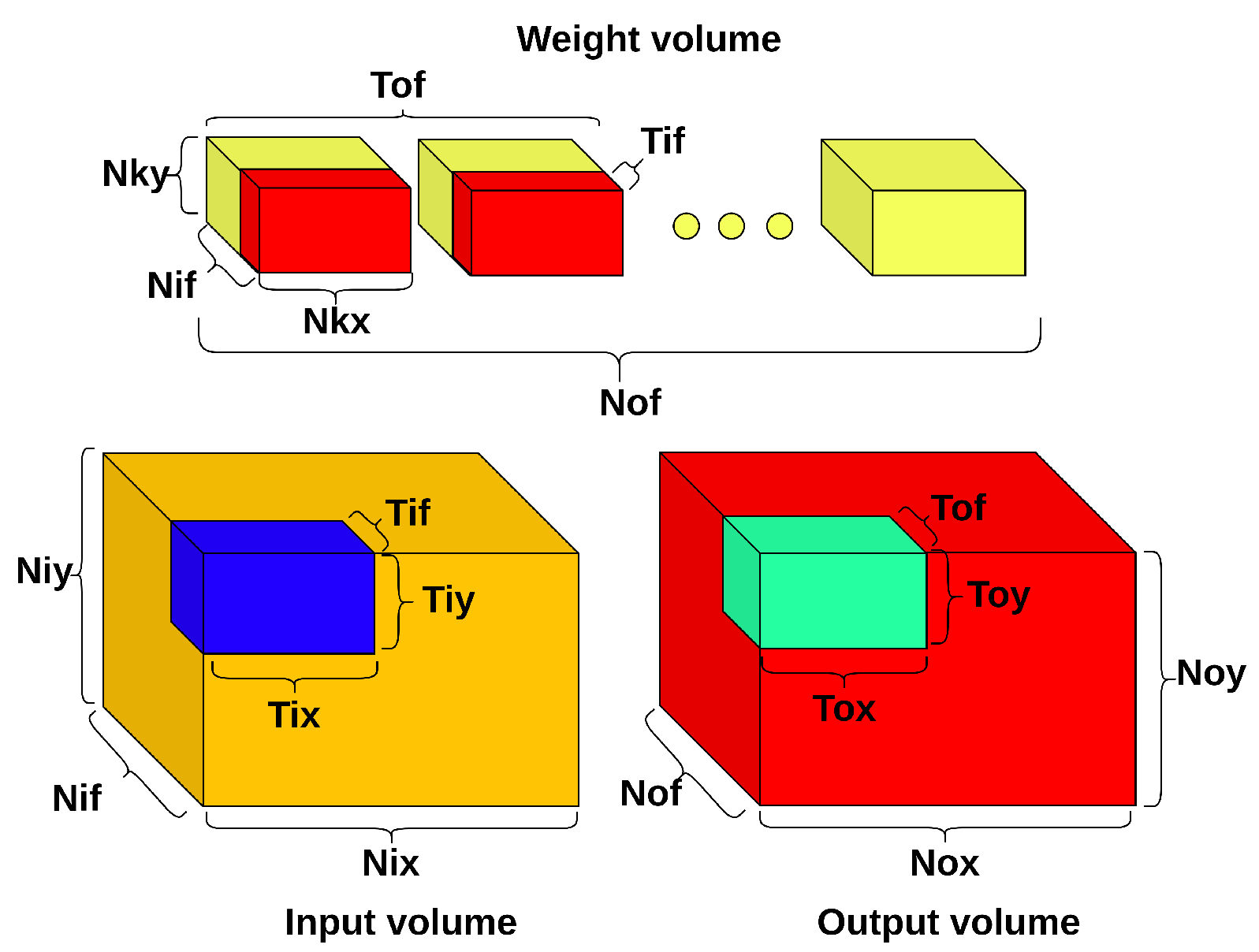
3. Background on Loop Scheduling

Modern architectures such as [6,7,19,20] have many reconfigurable settings that influence the performance, such as the computation energy and latency, and require a proper mapping. A loop schedule can be defined as a set of mapping parameters that characterize the communication and computation patterns of a hardware accelerator executing a certain workload. The methods used to optimize these patterns are called loop blocking techniques. They can be applied to any workload that can be represented as a series of nested loops, such as the generic convolutional layer in Algorithm 1 (notation reported in Table 1), with s denoting the stride, here, for simplicity, assumed to be equal for both the horizontal and vertical dimensions. The loop schedule of a convolutional layer for a target hardware accelerator defines the entire execution of a processing loop, such as after how many cycles a set of pixels is moved from one memory level to the other, or how many multiply and accumulate operations (MACs) are required to generate an output pixel with a certain set of processing engines (PEs).
Algorithm 1: Convolutional loop pseudocode.
Electronics 11 02933 i001
The objective of optimal loop scheduling is to maximize the data reuse in workloads with redundant computation, such as a convolutional layer. Typically, there are four reuse opportunities in the processing of a convolutional loop:
  • Input reuse: each input pixel is reused during the convolution to generate Nof feature maps;
  • Output reuse: each output pixel is reused during the accumulation of Nif feature maps;
  • Kernel reuse: kernel weights are reused Nox * Noy times over each input feature map;
  • Convolutional reuse: each input pixel is reused Nkx * Nky times for a single Hadamard product at a time.
There is an additional reuse opportunity that consists of reusing the intermediate pixel volume between layers. In this work, we named this reuse strategy inter-layer reuse, and it is detailed in Section 3.4.

3.1. Optimal Loop Scheduling on Dataflow Architectures

This work is focused on dataflow architectures, such as [6,7], often referred to as spatial arrays. Contrary to systolic arrays, where the computation patterns are fixed and scheduled by a main control, with no data reuse at the PE array level (no local memory except for I/O or datapath registers), spatial arrays leverage distributed control units to organize the data processing. Each processing engine has its internal control unit and register file; the latter is used to store input and partial results. A typical accelerator with a spatial array includes a memory hierarchy, normally composed of the system’s main memory (off-chip memory, DRAM), the internal main memory (on-chip memory, SRAM), and local memory, often implemented as a register file. Finally, point-to-point communication within the array of processing engines is managed by interconnections, often implemented as a network on chip (NoC). The overall architecture is depicted in Figure 1. The map-space on dataflow architectures is considerably larger than the one of systolic arrays because more hardware settings need to be configured [8,9]. The scheduling is usually carried out by minimizing cost functions that associate estimated performance metrics to the total data movement required to execute the workload [6,8]. These cost functions comprehend all significant energy and latency contributions due to data movement, such as MAC energy, memory read/write energy at every level, and communication through the NoC. Frameworks such as [8,9,10,11] create an abstract hardware model of the target accelerator and search the map-space by optimizing the aforementioned cost function for energy, latency, or both.
In this work, the target hardware accelerator is a spatial array with a row-stationary dataflow. The motivations behind this choice are the extensive documentation produced for this dataflow over the years [6,8] and its performance, which places row stationary as one of the most energy efficient dataflows found in literature [5]. In HW-Flow-Fusion, the same abstract hardware model defined in [8,11] is used to perform the dataflow mapping.

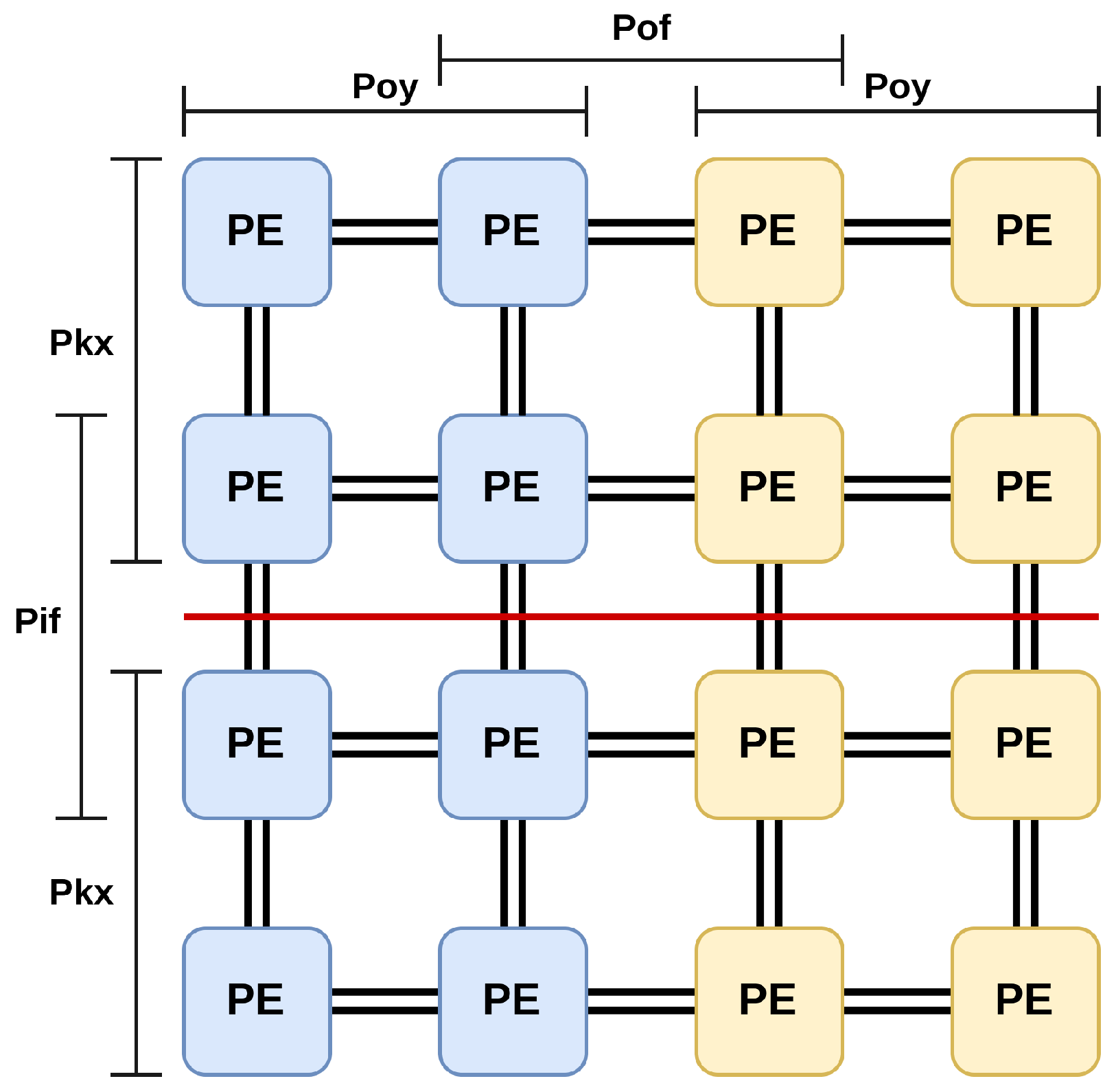
3.2. Temporal and Spatial Mapping

In order to simplify the analysis on the type of loop optimization performed at a particular memory level, two terms and definitions are borrowed from Timeloop [8]: temporal and spatial. Each memory level has a spatial and temporal mapping space; the loop blocking techniques detailed in Section 3.3 can be applied to both spaces and affect the mapping differently. When tiling is applied to a temporal level, it defines the amount of data moved between different memories within the accelerators’ memory hierarchy, whereas when it is applied to a spatial level, it defines the degree of unrolling. In this work, temporal tiling parameters are defined as tiling factors and spatial tiling parameters as unrolling factors. For loop reordering, when applied to a temporal level, it defines the order in which data are accessed at a specific memory level. When reordering is applied to a spatial level, it defines the dimension of unrolling over a hardware spatial dimension (height, width). In this work, we use temporal and spatial fusion to refer to layer fusion applied as a temporal tiling of the register file within the processing engines and as a spatial tiling over the dimension of the array, respectively.

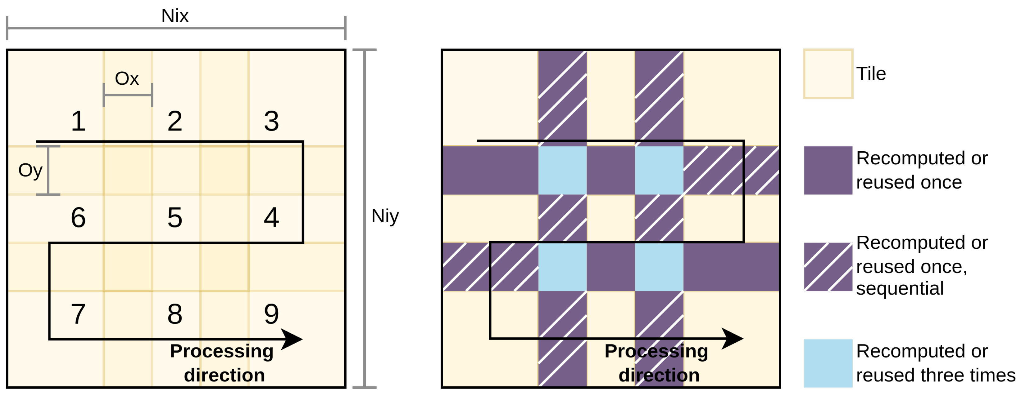
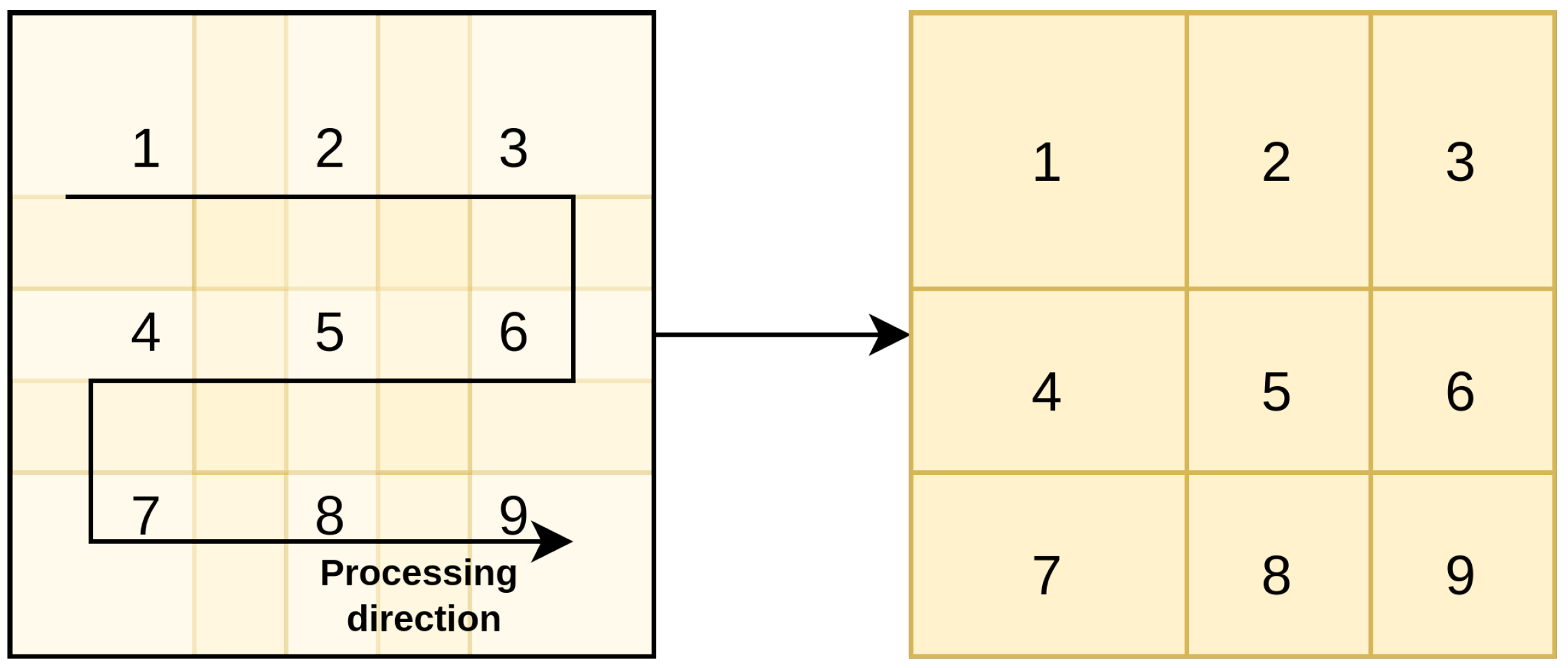
3.3. Loop Tiling and Reordering in Single-Layer Scheduling

Temporal tiling divides the data volume at a particular memory level in sub-volumes, as depicted in Figure 2. For each temporal tiling level, the memory footprint of the tiled volume identified with the tiling factors Tb, Tof, Tif, Tox, and Toy is defined as the buffer space required to store inputs, weights, partial sums, and outputs used during the computation. The memory footprint can be evaluated as shown in Equation (1). Precision here refers to the bit-width of the datatype.
I n p u t b u f f e r = T i x · T i y · T i f · T b · i n p u t _ p r e c i s i o n O u t p u t b u f f e r = T o x · T o y · T o f · T b · o u t p u t _ p r e c i s i o n W e i g h t b u f f e r = N k x · N k y · T i f · T o f · w e i g h t _ p r e c i s i o n
To check if a tiling set for a particular memory level is valid, the sum of the buffered volumes in (Equation (1)) must be less or equal to the total buffer size. The tiling set also defines the communication volume with the memory level above and depends strictly on the loop order. The loop order is correlated with different reuse opportunities, according to the relative position of nested loops. Considering the Algorithm 1, there are 120 possible permutations of the five outermost loops, but the possibilities can be reduced by analyzing the loop orders that significantly affect the communication. Although the frameworks [8,11] can support layer-wise loop reordering, only the original loop order described in [6] is considered to provide a well-documented baseline for single-layer scheduling. Therefore, only one loop permutation is described in this work. This particular loop order is defined as output reuse oriented in [16] since partial sums are never transferred to the main memory. It guarantees that all the output pixels are generated on-chip. The loop order of the convolutional loop pseudocode Algorithm 1 is an example of output reuse orientation. Equation (2) defines the unique fetch and write invocations of each buffered tile set in Equation (1).
I n p u t f e t c h = N i f T i f · N o f T o f · N o y T o y · N o x T o x · B T b W e i g h t f e t c h = N o f T o f · N i f T i f · N o y T o y · N o x T o x · B T b O u t p u t f e t c h = 0 O u t p u t w r i t e = N o f T o f · N o y T o y · N o x T o x · B T b
The total communication volume between two adjacent memory levels is then evaluated with Equation (3) and is the product of the invocation count (2) and the memory footprint (1).
T o t a l v o l u m e = I n p u t b u f f e r · I n p u t f e t c h + W e i g h t b u f f e r · W e i g h t f e t c h + O u t p u t b u f f e r · ( O u t p u t f e t c h + O u t p u t w r i t e )
Spatial tiling, or unroll, is used to partition the communication or computation across multiple buffers or processing engines at the same level of the memory hierarchy. Similar to temporal tiling, it is possible to have nested spatial tiling levels. For instance, in an accelerator such as the one in Figure 1, spatial tiling applied at the on-chip memory would partition the data stored in the memory banks for the computation and the space allocated to save the results. Nested spatial tiling applied at the PE level would unroll the computation of the data contained in the memory banks. For the effect of spatial tiling and reordering on a row-stationary dataflow, only the meaningful parameters are reported. The spatial loop order is fixed and the description and analysis can be found in [6,8], as they would be out of the scope of this work. Two parameters are relevant for the work presented in this paper, reported in Table 2, as they are influenced by the temporal and spatial tiling done during inter-layer scheduling: processing engine set (PE set) and unrolling. The values PEx and PEy represent the columns and rows of processing engines, respectively. A graphical representation of a possible mapping for a small processing engine array is depicted in Figure 3, on a 4 × 4 array with PEx = 4, PEy = 4, Pky = 2, Poy = 2, Pof = 2, and Pif = 2. Different colors represent different output channels; the red line separates different input channels. In Section 4.3 the array dimension is modified to fit multiple layers in the same array, constraining the spatial tiling factors to a subset of the initial single layer map space.

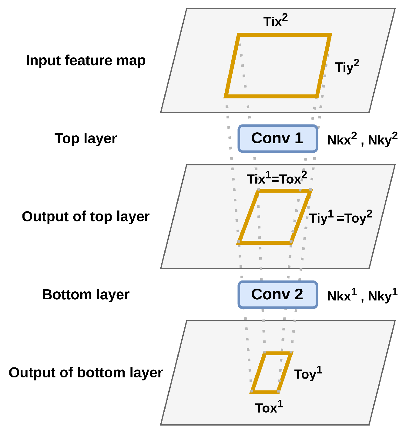
3.4. Inter-Layer Scheduling Concepts and Constraints

During the sequential execution of a convolutional layer on a typical HW accelerator such as [6,7,19,20], partial sums are accumulated to generate output pixels, which are then saved to the main memory, and then fetched again for the processing of the next layer, after the computation of the current one is finished. These output pixels, defined as intermediate pixels, could be fetched directly by the processing engines, along with the required set of filters, from the on-chip memory to compute the next layer’s output. This is the idea proposed for the first time in [12] and allows pipeline execution of layers by leveraging the reuse of intermediate pixels. Intermediate pixels are passed from one layer to the next and then discarded when they are no longer needed. Since CNN computation is deterministic, it is possible to evaluate the exact life span of input pixels, intermediate pixels, and sets of weights (i.e., for how long they should be kept in the on-chip buffer). All intermediate pixels exist only on the on-chip memory and are never transferred to the main memory, allowing additional energy saving by reducing the most expensive data movement, as the cost for DRAM accesses can be 20~30 times higher than that of SRAM accesses [6,8]. Moreover, by reducing access to the DRAM, it is also possible to reduce the communication latency and the impact of bandwidth bottlenecks on the computation [21].
In order to understand how inter-layer reuse can impact the communication efficiency, the normalized weight and pixel volumes for ResNet18 for ImageNet [2] are reported in Figure 4. Notice that pixel volumes dominate the first half of the CNN, whereas weight volume dominates the second one. Since inter-layer reuse depends on the volume of intermediate pixels, inter-layer scheduling can improve the hardware metrics only in some portions of the CNN, particularly where the volume is dominated by pixels. In this case, the execution of the first half of the CNN could be optimized by fusing layers, whereas the second half would be scheduled using traditional single-layer techniques since inter-layer reuse would be negligible.
All input/output pixels between the first and last fused layers are intermediate pixels, and the order in which they are generated is important; therefore, using different temporal loop reordering in inter-layer scheduling is not possible. As pointed out in Section 3.2, changing the temporal loop order affects the communication and computation pattern, resulting in a different order of pixel production and consumption for each layer, breaking the data dependencies.
The approach followed in this work is to create a batch-independent fusion schedule like the one proposed in [12], setting Tif = Nif and Tof = Nof for all the intermediate fused layers. This increases the buffering requirements (Equation (1)) significantly, with respect to scheduling with unconstrained input/output channel tile size, but eliminates two loops out of five per layer and grants maximum reuse per batch size because the buffered weights are reused during the computation of every Tox · Toy output pixels (Equation (2)). The fusion process occurs in a bottom-up fashion, starting from a set of output pixels in the last layer, defined as the bottom layer, and tracing back the computation to the first input layer, defined as the top layer. The output tile identifying the output pixels is propagated across all the layers between the top and bottom ones. Each time it travels across a new layer, due to the input–output relations, its feature size is increased. The set of Equation (4) describes the feature size transformations between two adjacent layers, m at the top and m 1 at the bottom, recalling that the input of layer m 1 is the output of layer m. The terms S x and S y denote the horizontal and vertical stride, respectively. A graphical representation of bottom, intermediate, and top tiling factor propagation on the spatial dimension of feature maps is depicted in Figure 5:
T o f m = T i f m 1 T o x m = T i x m 1 = ( T o x m 1 1 ) · S x m 1 + N k x m 1 T o y m = T i y m 1 = ( T o y m 1 1 ) · S y m 1 + N k y m 1 T i x m = ( T o x m 1 ) · S x m + N k x m 1 T i y m = ( T o y m 1 ) · S y m + N k y m 1
If temporal tiling is applied in a layer-fusion scenario, the same Equation (1) is applied for each layer within the fusion schedule. Layers in which the input is the output of the preceding one sharing the same buffer. Notice how the entire weight volume is allocated at once to allow the maximum batch reuse.
Intermediate buffers store both the previous layer’s output and the next one’s input. The evaluation of any layer scheduled in such a way can start only after enough output pixels have been evaluated. Intermediate buffers can be used to compute activation or normalization of layers between consecutive convolutional layers without additional storage. In [6], a similar solution is already implemented for activation layers. Therefore, ignoring shared buffers and assuming m = M as the top layer and m = 0 as the bottom one, the required buffer size is evaluated in Equation (5).
F u s i o n   b u f f e r = m = 0 M I n p u t buffer m + m = 0 M Weight buffer m + Output buffer bottom
The fetch and write invocations presented in Equation (2) can also be adapted, recalling that intermediate activations generate no external communication volume. The final communication volume is evaluated as in Equation (6); notice how weights are accessed precisely once, except for the bottom layer.
Total volume = Input buffer top · Input fetch + m = 0 M Weight buffer m + Output buffer bottom · Output write
One potential problem that can occur during layer fusion, as observed in [12], is that the intermediate pixels within adjacent tiles are re-computed again if not adequately buffered. This redundancy is present during standard processing and is described in the four reuse opportunities in Section 3. Figure 6 depicts the overlapping of the spatial dimensions of a feature map during the processing. The overlapping depends on the stride and the spatial dimensions of the tile, feature map, and kernel map. In [12], it is demonstrated that recomputation can account for up to 10 times the original energy cost estimated with single-layer scheduling; therefore, overlapping pixels must be stored in appropriate buffers. The overlapping regions Ox and Oy between adjacent tiles, depicted in Figure 6, can be evaluated as shown in Equation (7). In Section 4.1, a solution to the re-computing problem is presented, improving the one proposed in [12], from the observation that some overlapping regions are immediately reused during the computation.
O x = N k x S x O y = N k y S y

4. HW-Flow-Fusion: Inter-Layer Scheduling and Hardware Resource Optimization

Starting from the assumption that an accelerator based on a spatial array has enough hardware settings and control to support multiple processing sets to compute the same layer, as demonstrated in [6,7], in this work, we propose HW-Flow-Fusion, an inter-layer scheduling framework that can explore the map-space of fused layers. Instead of using dedicated arrays, we leverage the PE sets to compute different layers, reusing the available hardware resources.

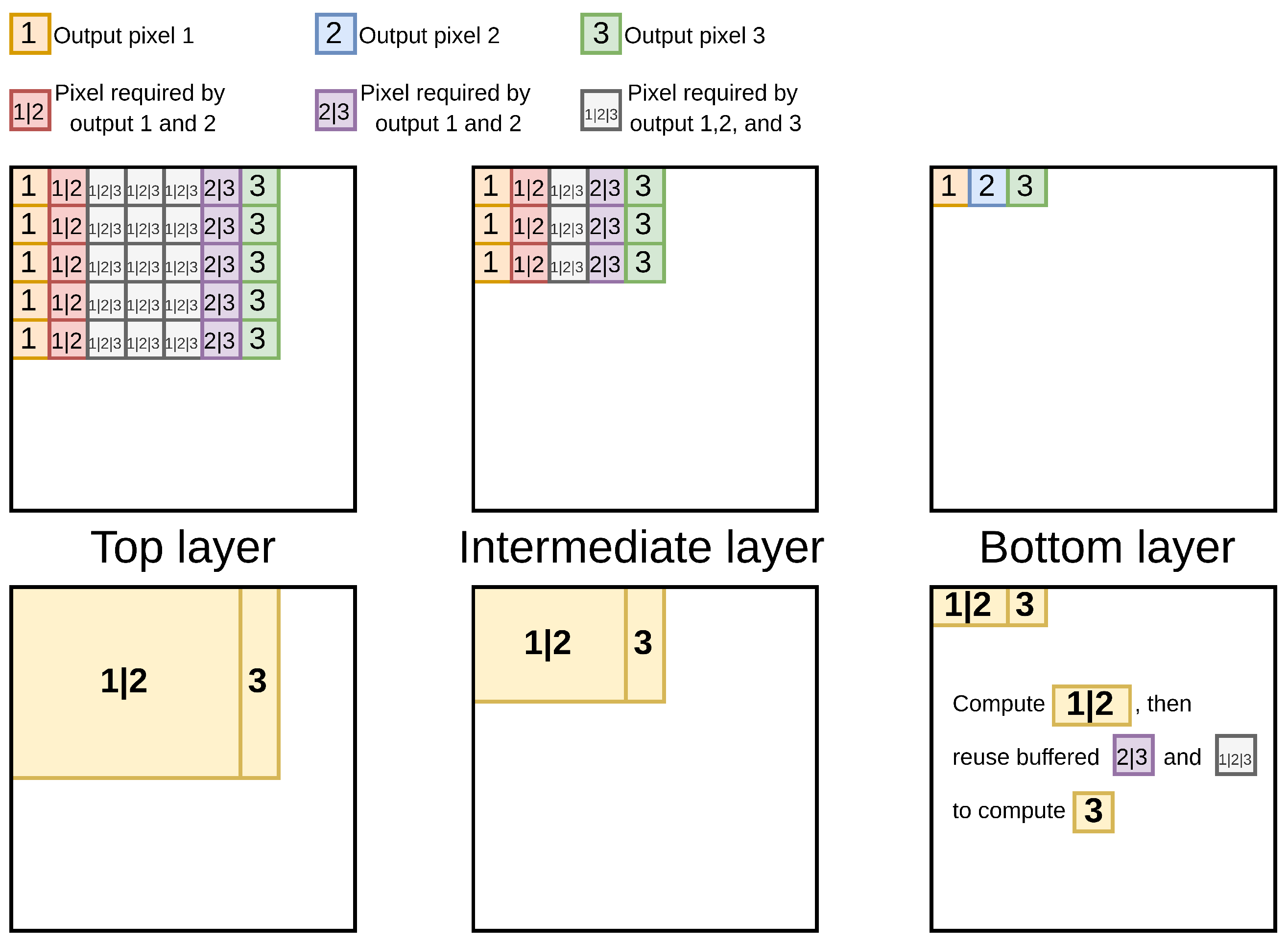
4.1. Optimized Intermediate Pixel Reuse Model

The problem of recomputation and the need for an appropriate reuse model was introduced in Section 3.4. The overlapping regions of Figure 6 indicate the tile portions that must be stored and reused to avoid recomputation. With appropriate tiling, it is possible to define the exact control sequence of a memory controller in charge of managing the correct movement of intermediate results between the processing units and the on-chip memory. This is the main reason for the proposed multi-tiling approach introduced in Section 4.2. Figure 7 depicts the overlapping regions, only one set of the regions to be stored and reused must be accounted for when evaluating the size of the reuse buffer. The required reuse storage is then given by Equation (8), the term reuse buffer x is used when the direction of tile processing is horizontal, as in Figure 6, and covers the contributions of (1,4), (1,2,4,5), (2,5), and (2,3,5,6), whereas reuse buffer y is used when the processing direction is vertical.
r e u s e b u f f e r x = ( N i x T i x ) · ( N k y S y ) · N i f r e u s e b u f f e r y = ( N i y T i y ) · ( N k x S x ) · N i f
The reuse model described in [12] additionally saves the sequential overlap, thus requiring extra storage that can be evaluated using Equation (9). In this case, reuse overhead y is for the horizontal processing and is added to the reuse buffer x , whereas reuse overhead x is for vertical processing and added to the reuse buffer y .
r e u s e o v e r h e a d x = ( T i x ( N k x S x ) ) · ( N k y S y ) · N i f r e u s e o v e r h e a d y = ( T i y ( N k y S y ) ) · ( N k x S x ) · N i f

4.2. Multi-Tiling for Minimum Reuse Memory with No Recomputation

Multi-tiling is used to schedule the computation of the exact amount of unique pixels needed for the current layer without generating redundant results. This technique, paired with reuse buffers, allows zero recomputation. Multi-tiling starts as a normal tiling process by generating a set of output tiles, Tox Toy, and then evaluating the corresponding input tiles, Tix and Tiy. To explain the multi-tiling process, a graphical example is depicted in Figure 8, in which the output pixels must be generated at the top, and intermediate layers are reported to produce the output pixels 1, 2, and 3 of the bottom layer. The computation was traced back using the input/output relations of Equation (4), assuming Nkx = Nky = 3, Sx = Sy = 1. With these values, a 3 × 3 input size is required to produce a single output pixel. Conversely, to compute a 3 × 3 intermediate tile size 5 × 5 input pixels are required. Let us suppose that the first tile to be evaluated is the one marked as 1|2 in the bottom right square. New unique pixels marked with 1, 2, 1|2, 2|3, and 1|2|3 are produced. From Equation (7) it is possible to evaluate the overlapping in the top and intermediate layer and store all the pixels that will be reused during the computation for output pixel 3, which are all the pixels marked with 2|3 and 1|2|3. Therefore, to compute the pixel number 3 in the bottom layer, the pixels marked with 3 in the intermediate layer must be computed. To do so, pixels 2|3 and 1|2|3 are read from the top-layer reuse buffer and used to generate the intermediate pixels, which are then processed with the pixels 2|3 and 1|2|3 read from the intermediate layer reuse buffer, to generate the final output value.
In order to reduce the amount of data saved in reuse buffers and justify the model proposed in Section 4.1, only unique pixels are scheduled for computation to reduce the overlapping. To produce new blocks of unique pixels in intermediate layers, the tile set must be shaped accordingly to exclude the recomputation of pixels stored in reuse buffers. If the previous example of Figure 8 is continued over the entire spatial dimension, the resulting tile sizes will look like what is depicted in Figure 9. These tiles are used to schedule the computation of new pixels every time they are executed. By comparing the left and right squares of Figure 8, it can be noticed that the tiles only cover pixels generated for the first time by every tile, minus the overlapping with the tiling factors that generated previous pixels. To define the spatial dimensions of these tiling factors, it is necessary to evaluate the three horizontal and vertical sizes from which it is possible to define the entire set. Naming the three horizontal sizes X1, X2, and X3, and the three vertical sizes Y1, Y2, and Y3, it is possible to define with Formula (10) the tile dimensions and occurrence, the latter, with the terms X r e p s and Y r e p s , represents the number of times a tile is repeated along the X or Y dimension.
X reps = ( Nox Tox 2 ) Y reps = ( Noy Toy 2 ) X 1 = Tix Px Y 1 = Tiy Py X 2 = Tix ( Nkx Sx ) Y 2 = Tiy ( Nky Sy ) X 3 = Tix 2 · Px X 1 X 2 · X reps Y 3 = Tiy 2 · Py Y 1 Y 2 · Y reps
The padding correction is necessary to avoid the scheduling of nonexistent pixels covering the borders of the feature map. Finally, it is possible to define in formula (11) the tile sizes, using the notation and position of Figure 9.
Tile   1 = X 1 · Y 1 Tile   2 = X 2 · Y 1 Tile   3 = X 3 · Y 1 Tile   4 = X 1 · Y 2 Tile   5 = X 2 · Y 2 Tile   6 = X 3 · Y 2 Tile   7 = X 1 · Y 3 Tile   8 = X 1 · Y 3 Tile   9 = X 3 · Y 3
The repetitions of these tiles depend on the size of Tox and Toy from which this set is generated. A possible set of tiles comprehend 1, 2, 3, 4, 6, or 9 valid tiles. In the case of nine valid tiles, the following tile matrix (12) represents the tile repetition across the feature map.
T i l e 1 T i l e 2 T i l e 3 T i l e 4 T i l e 5 T i l e 6 T i l e 7 T i l e 8 T i l e 9 = 1 X reps 1 Y reps ( Y reps · X reps ) Y reps 1 X reps 1
Finally, the total MAC computation with standard tiling and multi-tiling for a convolutional layer can be evaluated with Equation (13), the term Nif is set to zero for pooling layers. The total MAC operations for any layer is the same with both standard and multi-tiling.
compute standard = Nof · Nif · Nkx · Nky · Nox · Noy compute multi = Nof · Nif · Nkx · Nky · ( n = 1 9 Tile n · Repetitions n )

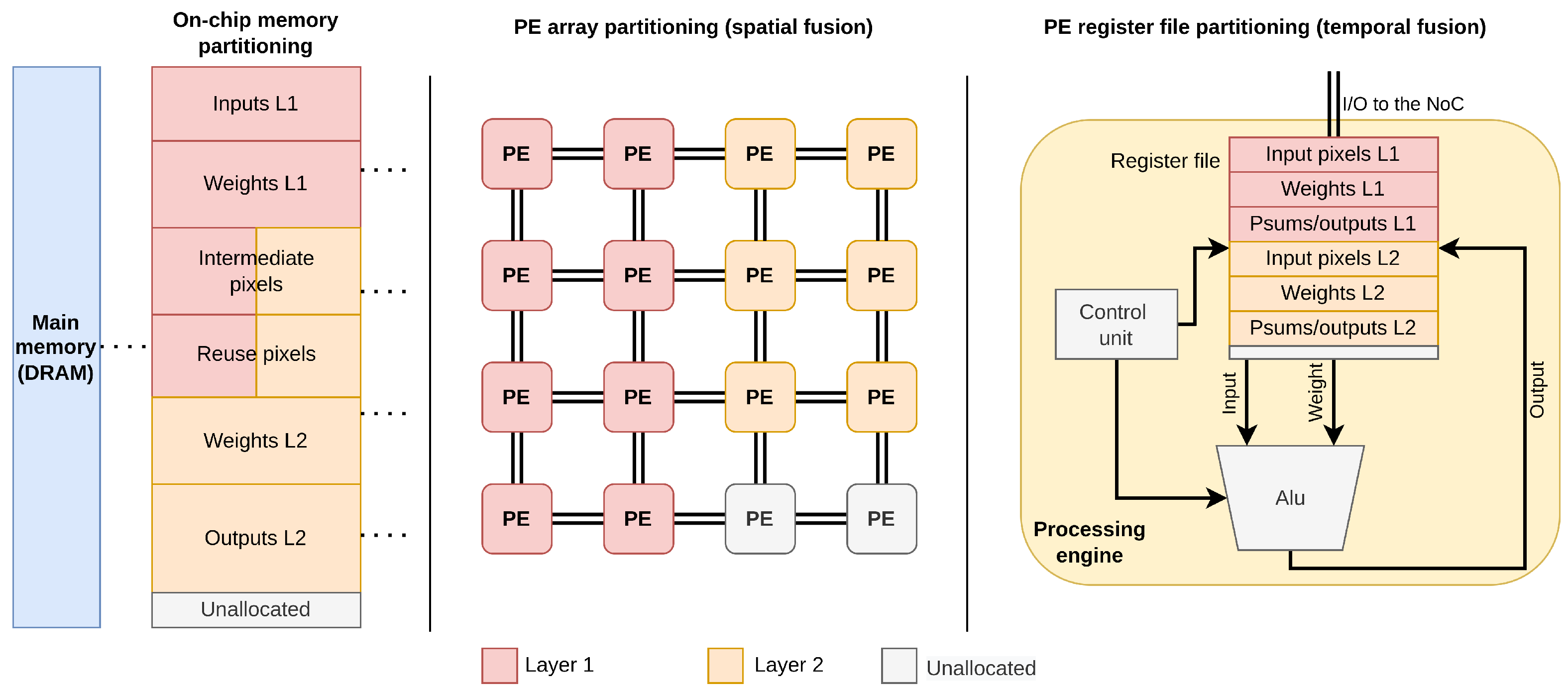
4.3. Hardware Resource Partitioning

The goal of a mapping framework such as Timeloop [8] or CoSA [9] is to find an efficient mapping for the target spatial array. This involves searching for optimal spatial and temporal tiling and reordering as detailed in Section 3.3. Resource partitioning is conducted at the layer level to map the execution of a single workload in [8,9,11], whereas resource partitioning in this work occurs at both the layer and the CNN level to map the execution of multiple layers on a fraction of the available resources. In this work, we explore both array and register file partitioning. The former is similar to spatial tiling at the array level (unrolling, PE set), and the latter is similar to temporal tiling at the register file level (loop tiling). Figure 10 depicts the spatial and temporal fusion proposed in this work and detailed in the following paragraphs. Since the main focus is the analysis of inter-layer scheduling opportunities, an analysis of the required high-level and PE-level control is omitted.

4.3.1. Spatial Fusion

Spatial fusion is the partitioning of the PE array for the computation of multiple layers sharing the same on-chip memory and reuse buffers. This partitioning models an accelerator in which the PE array can be divided into smaller regions, each computing a different layer and communicating with the on-chip buffer to read and store the data. Each PEs region would compute the output pixels of the layer assigned to it and send them back to the on-chip memory, which would be read by another PEs region that would compute the output pixels of another layer and repeat the same process. The objective of spatial fusion is to find the size of sub-arrays like those depicted in Figure 10, which can achieve an energy-efficient or high-throughput scheduling. It is impossible to know the best partitioning beforehand, as any combination of sub-arrays with any widths and heights could be the optimal one. Therefore, analyzing each combination and comparing the loop schedules is necessary to find the most efficient resource allocation. It is important to highlight that each sub-array will execute only one layer within the fusion schedule, so the partitioning must assign the best amount of the resource to each workload, with the number of sub-arrays equal to the number of layers fused. To find the best partitioning for N number of layers, we start by evaluating all the N sub-arrays that can fit within the original PE array without overlapping, using the method described in [22] to remove illegal solutions. Only sub-arrays of height and width that are even divisors of the PE array dimensions are considered to prune the large solution space, which is then reduced again by removing solutions that are known to be illegal for certain dataflows. For instance, recalling Table 2, when mapping on a row-stationary dataflow, it is possible to remove all arrays with a height that is smaller than the horizontal dimension of the kernel, as they would not generate any legal mapping, as detailed in [6]. Finally, each tile set of every fused layer is mapped for each combination of sub-arrays, and hardware metrics are collected and compared to find the most energy/throughput-efficient partitioning. A possible downside of spatial fusion is that the unrolling factors of the fusion schedule might be smaller than those of a single-layer schedule, being constrained by the sub-array sizes, which might result in increased computation latency.

4.3.2. Temporal Fusion

Temporal fusion consists of partitioning the register files (RF) of each PE in the array for each layer within the fusion schedule. This partitioning models an accelerator in which the register file inside the PEs can be used to store input, weight, and output pixels belonging to different layers and process them alternatively. To some extent, this could be similar to CPU multi-threading, which allows the same core (PE) to process multiple threads (layers) sharing the same cache (register file) and datapath (MAC). The execution of a layer would be paused when there are not enough input pixels to compute a partial sum or output pixel and the PE would switch to compute another layer with the data available in the register file. Theoretically, this can reduce the PE idle time as it would always have multiple jobs to process. A possible downside of temporal fusion is that the interleaving search space is reduced by reducing the register file size assigned to each layer. Interleaving is leveraged by some dataflows such as row-stationary in [6] and output-stationary in [19] to compute partial sums of multiple output channels within a single PE, reusing the same input data with different kernels. On the other hand, according to [23], the register file size does not significantly impact the performance, while the PE array size does, so the reduction in interleaving possibilities should not degrade the efficiency. At the same time, the possibility to unroll the execution of each layer over the original array size (compared to spatial fusion) should result in lower computation latency and higher energy efficiency, as both strictly depend on the number of PEs and the possibility to have larger spatial tiling factors (not constrained in temporal fusion). In the hardware model adopted by this work and [8,11], the register file of a certain PE is divided into three sections: one for the weights, one for the inputs, and one for the partial sums. In inter-layer scheduling, each of these sections has to be partitioned into N sub-sections, with N being the number of fused layers. The search space is limited to one combination for each fusion schedule, which is obtained by dividing the input, weight, and partial sums register file into N sub-sections, respectively. For instance, the register file of a standard row-stationary model accelerator in [8,11] is divided into 384 bytes for the weights, 24 for the input pixels, and 36 for the partial sums. In case of a fusion schedule with two layers, with N = 2, each layer would have 192, 24, and 36 bytes for the weights, input pixels, and partial sums, respectively.

4.4. Proposed Inter-Layer Scheduling Framework

The inter-layer scheduling framework HW-Flow-Fusion is built on a validated tool named HW-FlowQ [11] and reuses it as it is for single-layer scheduling. The framework is written in Python and uses Tensorflow 1.13 for the definition of CNNs models. The framework used in this work is depicted in Figure 11 and is composed by several blocks, two of which execute some tasks that have been described in previous sections. Valid hardware resource partitions for spatial and temporal fusion are evaluated as explained in Section 4.3. Tile sets are evaluated as detailed in Section 4.2 using Equations (10)–(12), whereas buffering requirements are evaluated with Equations (5) and (8), as explained in Section 4.1.
The procedure to generate and map the sequence of fused layers begins with the evaluation of sequences of layers that can be fused with the available hardware resources. Starting from a sequence composed of a minimum of two layers, all possible tile sets are evaluated and used to check the validity of the fusion schedule, comparing the total allocated memory with the buffer size. The solution is marked as legal and saved for further evaluation if the total memory occupation is less than or equal to the available memory size. If at least one valid solution exists for the current sequence of layers, a new adjacent layer is added to the sequence, and the validity check process starts over with an additional layer, and this process continues until there are no valid sets for a sequence. When this happens, the cycle starts again with a new sequence composed of the first layer that could not be fused and the next. Multiple layers can be included in different fusion schedules. For instance, if the first four layers of a CNN can be fused, this procedure outputs three legal fusion schedules: one for the first two layers, one for the first three layers, and one with all four layers. This process continues until the entire CNN has been analyzed and outputs a set of sequences and single layers, which compose the solution space searched by the scheduling framework. The scheduler receives the corresponding layer dimensions, tile sets, and buffer/RF/array partitions for each sequence of fused layers or single layers. Each solution is then evaluated, hardware metrics are generated, the fused sequences are compared against each other, and the corresponding layers are scheduled singularly. Only the fusion schedules that improve the target hardware metrics with respect to single layers are included in the final output. The hardware metrics are evaluated using the same architecture model and energy/delay models of Timeloop [8] and HwFlowQ [11]. The target hardware platform is an ASIC spatial array, configurable with different dataflows and memory hierarchies, with a typical structure as the one depicted in Figure 1. The energy and delay of each operation (MAC operation, RF read, NoC transfer, etc.) are multiplied for the total access count specific to that resource. For instance, the DRAM energy for each operation is multiplied for the write access count evaluated as Outputwrite in Equation (3).

5. Results

For all experiments, we used the energy model of [8,11] and six hardware configurations of a spatial-array accelerator, where the model architecture is based on Eyeriss [6], reported in Table 3 and Table 4. For each configuration, the batch size is one, the dataflow is row-stationary with the same loop order used in the original Eyeriss accelerator [6] and also in Timeloop [8] for single-layer scheduling, the MAC precision is 8 bit, and its energy cost comprehends the MAC contributions plus two memory read operations, and one memory write operation from/to the register file. Each memory access is evaluated as the cost of the read operation from the source plus one write operation to the destination. The on-chip buffer bandwidth is 2 bytes per cycle, and the DRAM burst length is 8 bytes. The refined computation to communication ratio (CTC) formula proposed in Caffeine [21] is used to evaluate the communication efficiency.

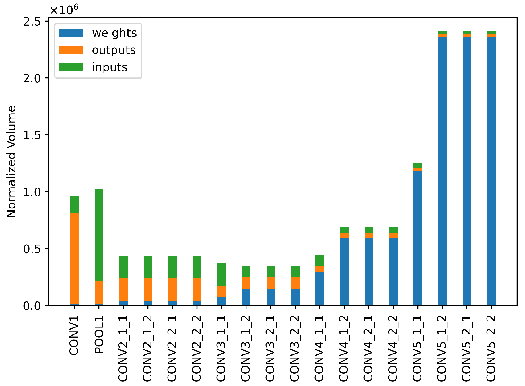
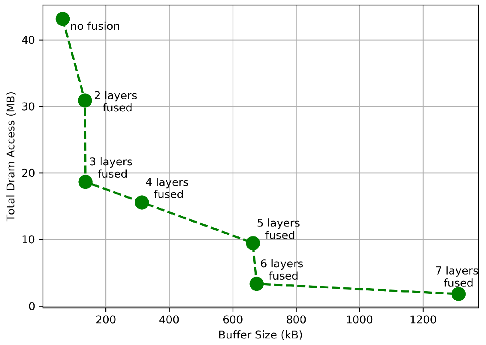
5.1. Reuse Buffer Comparison and Impact of On-Chip Memory on Layer-Fusion

The memory required to fuse multiple layers depends on the constraints Nif = Tif and Nof = Tof that both this work and [12] apply. In order to fuse two or more layers, the entire weight volume must be stored on-chip. In Figure 12, it is possible to see how the on-chip storage affects inter-layer scheduling. In order to replicate the results from [12] and make a fair comparison, the CNN tested is VGG16-E [1], with all layers and data quantized to 16 bit. We consider the first seven layers of the CNN, which are CONV1-CONV2-POOL1-CONV3-CONV4-POOL-CONV5. Notice how the DRAM communication volume is reduced by ~60% when fusing the first three layers. There is almost no difference in memory requirements when fusing three or six layers, because the third and sixth layer of both schedules would be a pooling layer, which requires no weight memory.
The reuse model proposed in Section 4.1 is an improvement over the one proposed in [12], which is used as the baseline in the comparison of Figure 13. The additional buffer memory is evaluated as kB of reuse buffer that must be allocated to achieve zero recomputation. The reuse model presented in this work outperforms [12], requiring from ~15% to ~22% less additional memory than [12] when fusing the same number of layers and achieving the same reduction in communication volume. The gap becomes even wider when the number of fused layers increases because deeper layers have more feature maps, and the size of each sequential overlap that must be stored with the reuse model [12] increases.

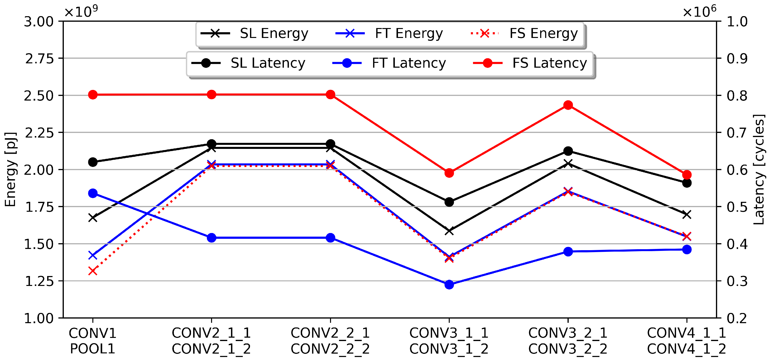
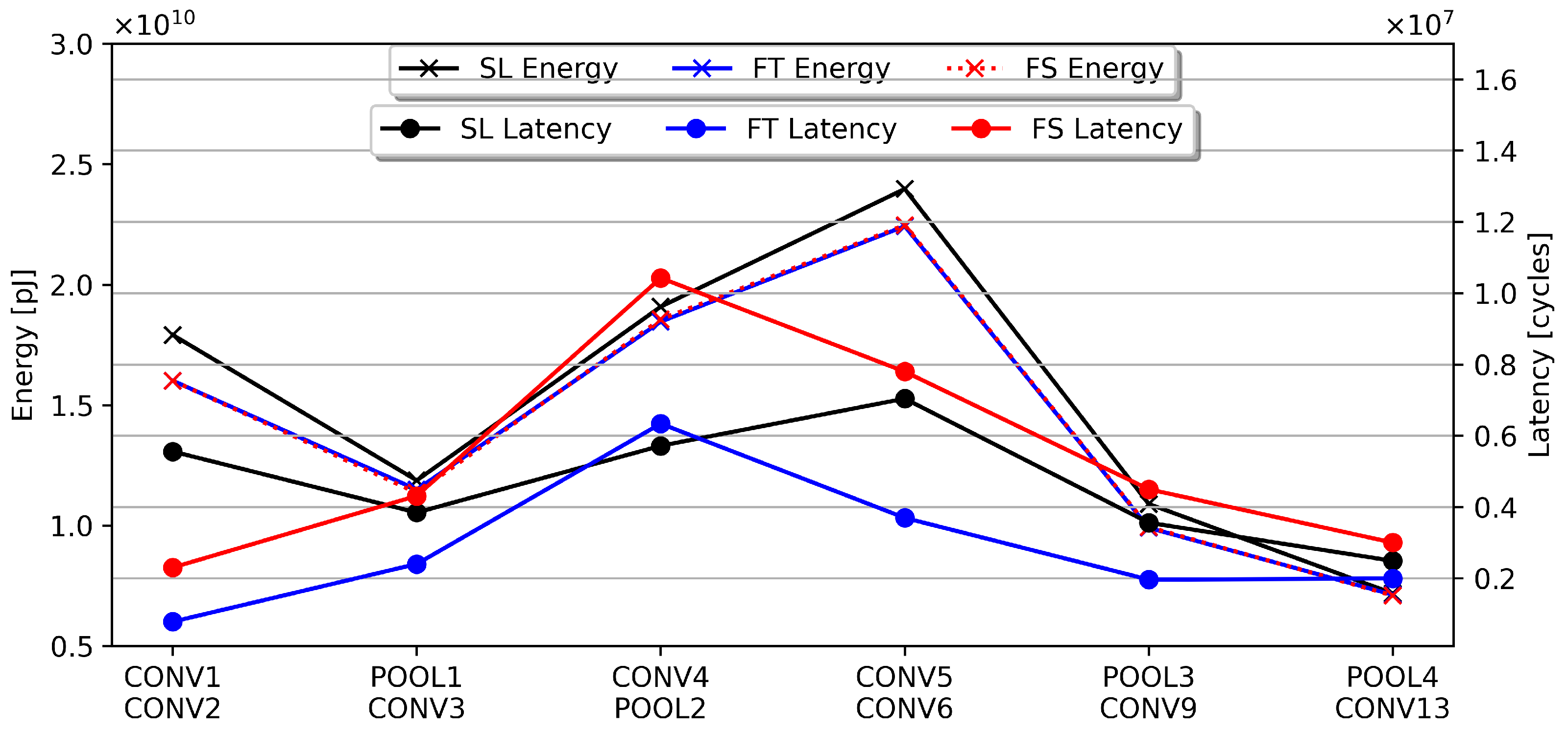
5.2. Comparison of Spatial, Temporal Fusion, and Single Layer Hardware Metrics

We compare the HW metrics estimated with standard scheduling, here named single-layer, against those generated with inter-layer scheduling. For this experiment, we use ResNet18 and VGG16-E, HW configuration 1 of Table 3 and set the maximum number of fused layers to two. We only compare layers included in fusion sequences since the framework outputs the same mapping for the layers that cannot be fused. The energy and latency estimates for ResNet18 are reported in Figure 14, those for VGG16-E in Figure 15, the overall energy and latency ratios are reported in Table 5, evaluated as the sum of the contributions for each layer in the sequence. Only six couples of layers could be fused with this hardware configuration because the on-chip buffer size limits fusion possibilities once the number of feature maps starts to increase in deep layers. For VGG16-E, the buffer size prevents the fusion of any layer after the sixth, but there are two max poolings (zero weight memory) that precede two convolutional layers, which allow the scheduler to find two additional fusion sequences. For ResNet18, it is possible to fuse couples of consecutive layers up to the twelfth convolutional layer.
From the collected results, it is possible to see that temporal fusion can reduce the energy, latency, and communication volume for almost every sequence, while spatial fusion can only improve the energy and communication volume with a significant increment of the latency. With temporal fusion, the overall latency is reduced to 66% for ResNet18 and to 61% for VGG16. For ResNet18, the latency reduction is consistent through the six couples of fused layers, whereas with VGG16-E, the gap with single-layer schedules is smaller. On the other hand, spatial fusion can match or slightly improve the energy with respect to temporal fusion. The major contribution to latency is due to the computation rather than communication, as spatial fusion achieves approximately the same communication volume as temporal fusion. As anticipated in Section 4.3, a rise in the computation latency was to be expected as it strictly depends on the unrolling and available PE engines. By analyzing the results reported in Figure 14 and Figure 15, it is possible to conduct the same observations in [23] regarding the accelerator architecture design choices for high throughput, which is that the number of PEs is more important than the size of the register file within each PE. Recall that temporal fusion uses the entire PE array and reduced register file for each layer, whereas spatial fusion uses reduced PE arrays and the entire register file for each layer. In this experiment, the scheduler found the array partitioning reported in Table 6. The array partitioning search space is limited to sub-arrays with spatial dimensions that are divisors of the original PE array size, whereas the register file partitions are fixed to 1 N of the original size, with N being the number of layers within the fusion sequence. It is possible to notice that the layers scheduled with spatial fusion are executed using partitions that are half of the original PE array size, with one exception for the first two layers of VGG16-E, where one quarter of the original array is assigned to each layer. Therefore, for spatial fusion, the communication latency improvement achieved with inter-layer scheduling is lost due to the higher computation latency resulting from executing each workload on fewer PEs with respect to the single-layer scheduling approach.
The energy consumption of spatial and temporal fusion is marginally improved with respect to the single-layer because only the communication energy is improved with the inter-layer scheduling method presented in this work. Further investigation of inter-layer scheduling could focus on reducing data movement between the register file and on-chip buffer by directly forwarding computed output pixels from one processing engine to another. The major contributions to the overall energy consumption come from the data movement within the PE array and the on-chip memory accesses, as demonstrated in [6,8]. Moreover, the overall communication volume required to process the layers reported in the figures is halved for both CNNs. The results for VGG16-E could have been anticipated by observing Figure 12. With CONV1 and CONV2 fused, the communication volume is reduced by ~25%, with POOL1 and CONV3 by ~10%, and with layers CONV4 and POOL2 by ~17%. While there are three more couples of fused layers in the VGG16-E experiment of Figure 15, the pixel communication volume is dominated by the six layers we just mentioned.
Finally, we analyze the improvements in the CTC ratio, recalling the definition and analysis from [21]. The peak performance of an HW accelerator is bounded by either the computational rooftop (theoretical maximum number of operations per cycle) or the system’s memory bandwidth multiplied by the CTC ratio. The memory bandwidth limits the accelerator’s performance because for each functional unit (in our case, the PEs) to work at full regime, it must be continually fed with data from memory. The CTC ratio defines the amount of computation attainable with a certain amount of communication. Recalling that there are four reuse opportunities in single-layer scheduling and an additional one in inter-layer scheduling, the CTC ratio can be increased by maximizing data reuse and reducing data movement between different memory levels. In this case, inter-layer scheduling could outperform the single-layer as it completely removes the off-chip communication between intermediate layers. The CTC ratios for standard and fused scheduling are reported in Table 7. The increment of the CTC ratio is more noticeable in layers dominated by pixel volumes, such as the first couple of layers of VGG16-E, and generally in fusion sequences containing a POOL layer at the end.
To understand why the CTC ratio worsens for deeper layers, we must recall that the refined CTC ratio used in [21] also depends on the burst length and, therefore, how much continuous data are read from the off-chip memory. Therefore, moving multiple small sequences of pixels might be worse than moving a few large sequences, as the latter would use the memory bandwidth more efficiently than the former. Considering that we set the constraints Tif = Nif and Tof = Nof for all intermediate layers, forcing the scheduler to save the entire weight volume inside the on-chip buffer, there is not much storage left to store intermediate pixels. Therefore, the tiling factors composing the tile sets of layers with a high number of feature maps tend to be smaller, resulting in a communication pattern made of small memory read and write operations. This increases the communication latency and reduces the memory bandwidth efficiency. Moreover, when using the multi-tiling approach proposed in Section 4.2, the tile sets used to block the processing of pixels around the center of the feature map spatial dimensions are inherently smaller than the others and might not use all the available on-chip buffer. Currently, our scheduler selects the biggest tile set, i.e., the one with the largest memory footprint, to perform the legality check of the fusion schedule. These small tile sets are what allow for fusing layers with zero-recomputation but are not bandwidth-efficient when their sizes are too small. A possible solution to taper this inefficiency could be to regroup the tile sets with a repetition count higher than one, in particular, referring to formula (11), tile 2, 4, 5, 6, and 8. Regrouping small tile sets could allow the movement of more data between the off-chip and on-chip memory, resulting in a fusion schedule with a smaller degradation of the bandwidth efficiency. We leave this study as future work.
Overall, temporal fusion can achieve lower latency, energy, and communication volume with respect to a single layer schedule, outperforming spatial fusion. Furthermore, temporal fusion computation latency is not penalized by a smaller PE array partitioning as spatial fusion, whereas the latter trade-off latency had slightly better energy efficiency and increased CTC ratio. These results prove that inter-layer scheduling can improve dataflow-based CNN accelerators’ performance metrics.

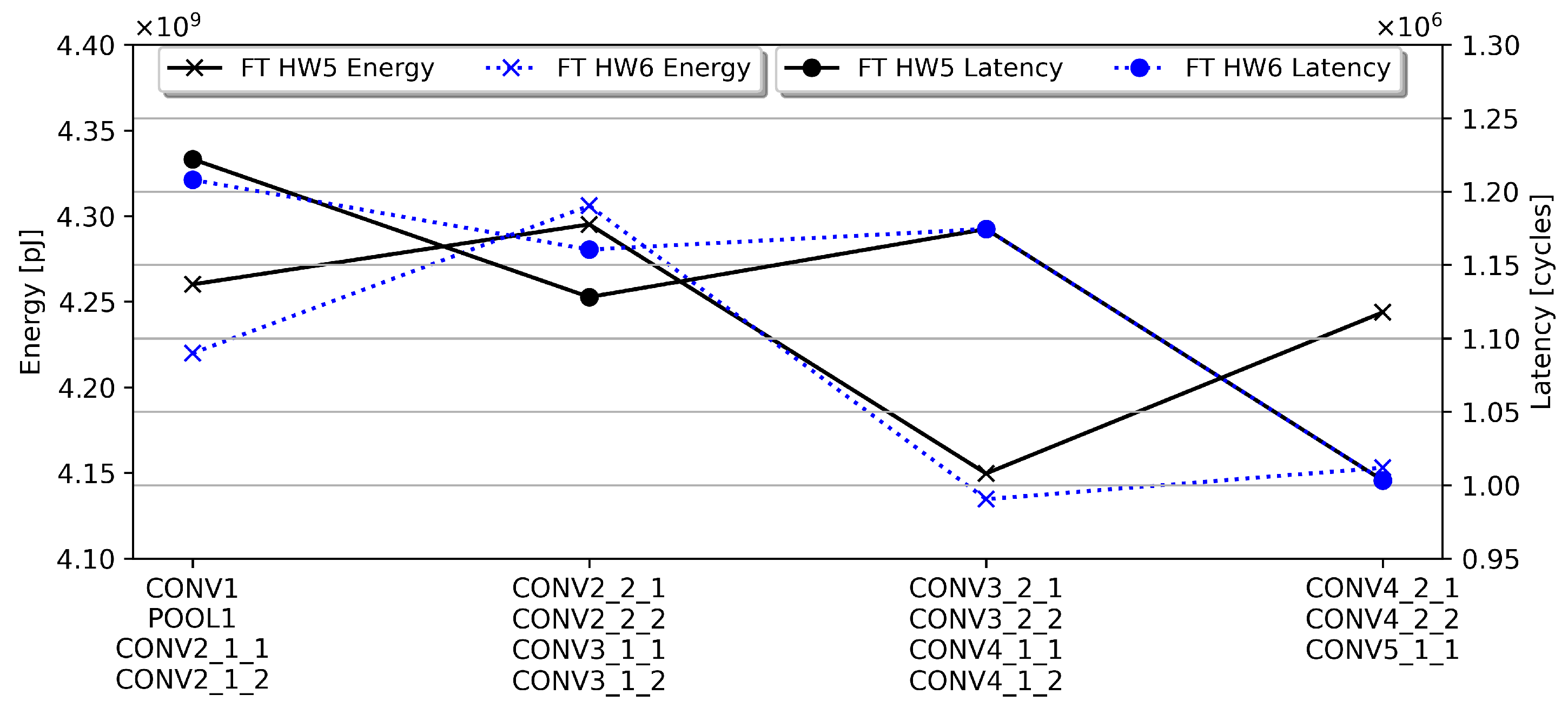
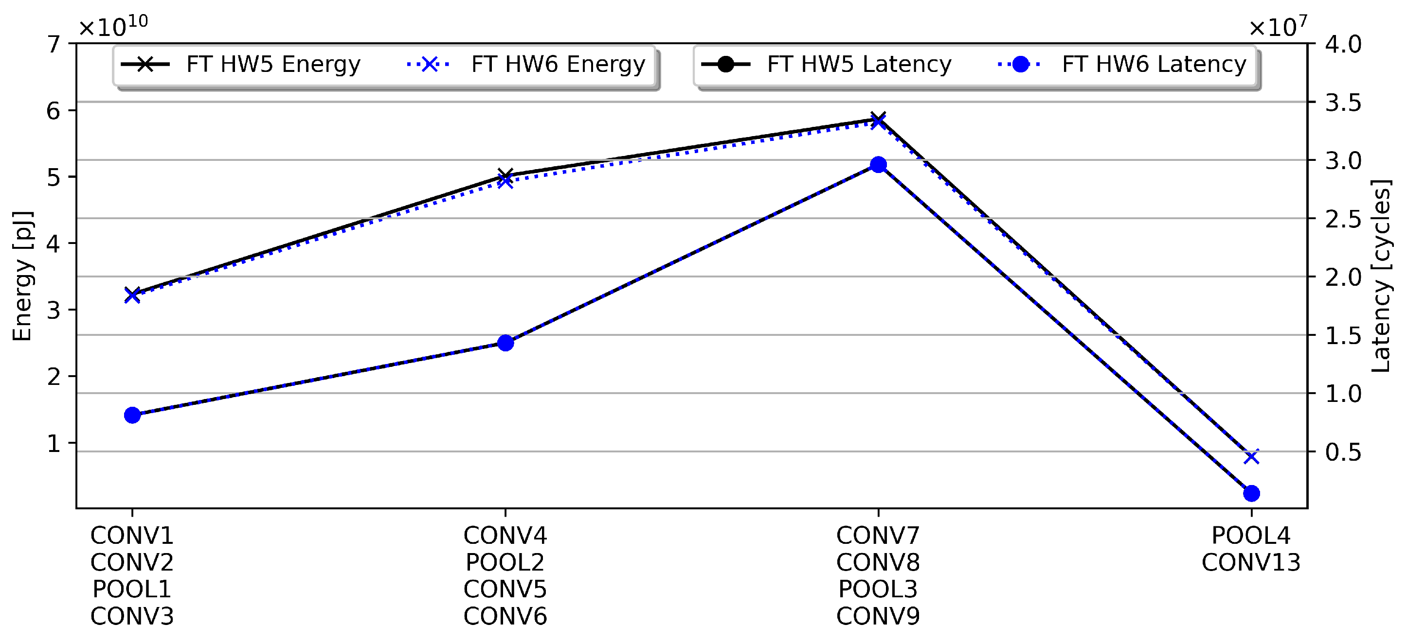
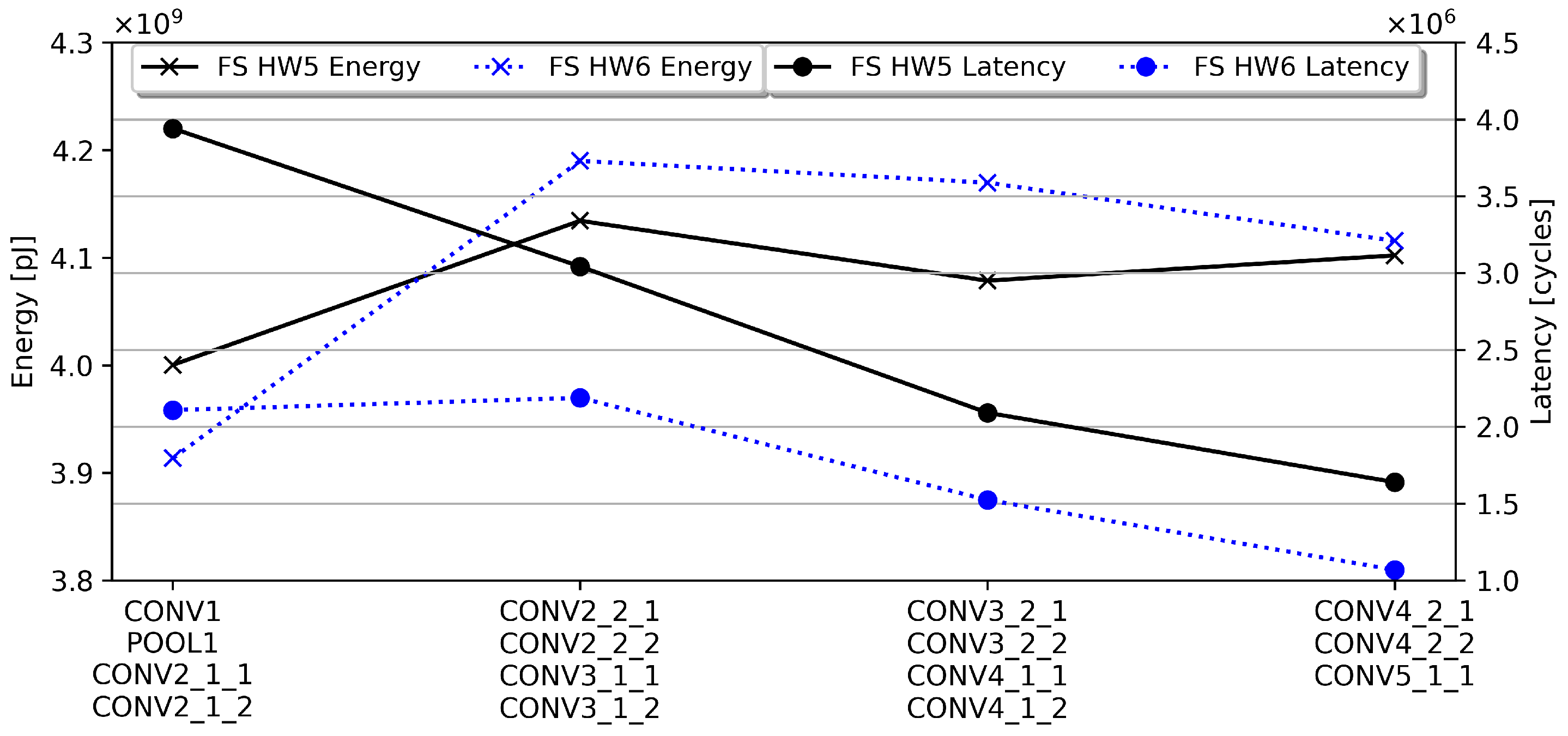
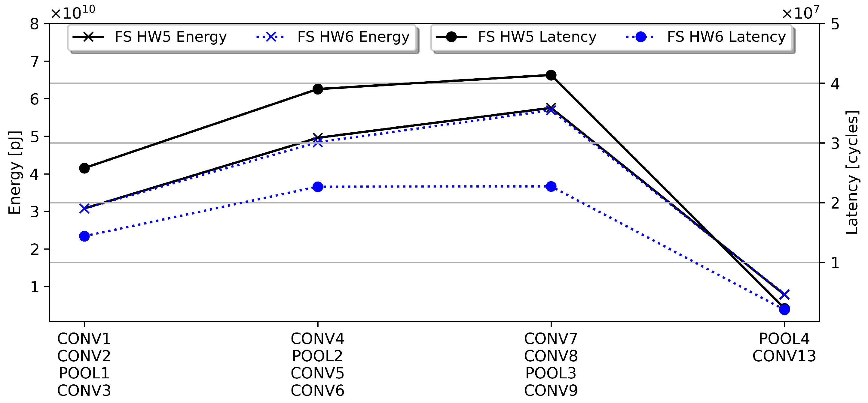
5.3. Hardware Constraints and Scaling on Inter-Layer Scheduling

In this section, we experiment with different HW configurations to understand how layer fusion performance scales with different HW resources. In particular, two HW configurations (3 and 4 of Table 3) are used to measure if spatial fusion can leverage the additional processing engines obtained by increasing the array size when fusing, at most, four layers. Similarly, the two HW configurations, five and six, are used with temporal fusion for the same purpose, with additional register file memory for each PE with sequences of maximum four layers. The on-chip buffer is over-dimensioned for the two CNNs considered. In both experiments, it was set to 1536 kB to increase the solution space explored by the inter-layer scheduling framework, relaxing the legality checks while evaluating the sequences of layers that can be fused.
We start by analyzing the results with temporal fusion in Figure 16 for ResNet18 and Figure 17 for VGG16-E. The size of the register file within each PE in HW configuration six was increased by 50% with respect to HW configuration 5. Therefore, the scheduler can fuse at least four layers for both configurations, with a minimum RF memory-per-layer equal to or higher than the one allocated for two layers with HW configuration 1. The results clearly show that there is no performance scaling when the register file size is increased since the energy and latency metrics with HW5 and HW6 of Table 3 are less than 1% for energy, latency, and CTC ratio. This experiment confirms that register file size does not significantly influence the energy or throughput efficiency of an accelerator and is congruent with the observations made in [23].
For what concerns the performance scaling with spatial fusion, reported in Figure 18 and Figure 19 for ResNet18 and VGG16-E, the overall energy difference for both CNNs with both HW configurations is in the range of ±1%. Again, no noticeable improvement in energy efficiency was achieved by scaling the PE array size. On the other hand, the latency was significantly improved, with a 45% latency reduction between HW config. 5 and 6 for ResNet18 and 75% for VGG16-E. These results are again congruent with the observations made in [23] and prove that spatial fusion can benefit from additional PEs. A larger PE array means that the scheduler can unroll the execution of each layer over larger partitions, reducing the constraints on the unrolling factors, resulting in a much lower computation latency.
In conclusion, of the two fusion methodologies proposed in this paper, temporal fusion proved to be the best choice for small accelerators such as the one modeled in HW configuration 1 but does not scale with additional resources. In contrast, spatial fusion is severely limited on small PE arrays; however, it might be the best option to improve the computing performance on large accelerators, such as those modeled with HW configurations 3 and 4.

6. Conclusions

Energy- and latency-efficient CNN acceleration is achieved by leveraging different scheduling techniques to minimize data movement and maximize reuse. In this work, we present an inter-layer scheduling framework that can exploit intermediate pixel reuse, alongside the other common reuse strategies used in previous works. Furthermore, we investigate the constraints and trade-offs of layer fusion and provide a mathematical background to understand how to map the execution of multiple workloads with data dependencies on the same HW accelerator. Finally, we propose an improved data reuse model, tiling, and partitioning strategies that allow fusing multiple layers without recomputation on generic spatial array accelerators. As further work, the proposed inter-layer scheduling method could be included in standard single-layer scheduling frameworks and optimized to improve the solution space and search efficiency. Moreover, inter-layer scheduling could be investigated even further to move layer fusion at the dataflow level to reduce some of the current limitations on the sequences of layers that can be fused, and further optimize data movement. Compared to standard scheduling techniques, the two fusion strategies, named spatial and temporal, can reduce the communication volume by 51% and 53% for VGG16-E and ResNet18 on a spatial array accelerator and reduce the latency by 39% and 34%, while also increasing the CTC ratio, resulting in a better memory bandwidth efficiency.

Author Contributions

Conceptualization, E.V., P.M., N.F., M.R.V. and A.F.; methodology, E.V.; software, E.V., N.F. and M.R.V.; validation, E.V., N.F. and M.R.V.; formal analysis, E.V.; investigation, E.V.; data curation, E.V. and P.M.; writing—original draft preparation, E.V. and P.M.; writing—review and editing, E.V., P.M., N.F., M.R.V., A.F. and L.F.; visualization, E.V., P.M., N.F. and M.R.V.; supervision, M.M., G.M., C.P. and W.S.; project administration, M.M., G.M., C.P. and W.S. All authors have read and agreed to the published version of the manuscript.

Funding

This research received no external funding.

Data Availability Statement

Not applicable.

Conflicts of Interest

The authors declare no conflict of interest.

Abbreviations

The following abbreviations are used in this manuscript:
CNNConvolutional neural network
HWHardware
PEProcessing engine
RFRegister file
NoCNetwork on chip
CTCComputation to communication
MACMultiply and accumulate

References

  1. Simonyan, K.; Zisserman, A. Very deep convolutional networks for large-scale image recognition. arXiv 2014, arXiv:1409.1556. [Google Scholar]
  2. He, K.; Zhang, X.; Ren, S.; Sun, J. Deep residual learning for image recognition. In Proceedings of the IEEE Conference on Computer Vision and Pattern Recognition, Las Vegas, NV, USA, 27–30 June 2016; pp. 770–778. [Google Scholar]
  3. Tan, M.; Pang, R.; Le, Q.V. EfficientDet: Scalable and Efficient Object Detection. In Proceedings of the 2020 IEEE/CVF Conference on Computer Vision and Pattern Recognition (CVPR), Seattle, WA, USA, 14–19 June 2020; pp. 10778–10787. [Google Scholar] [CrossRef]
  4. Gidaris, S.; Komodakis, N. Object detection via a multi-region and semantic segmentation-aware cnn model. In Proceedings of the IEEE International Conference on Computer Vision, Santiago, Chile, 7–13 December 2015; pp. 1134–1142. [Google Scholar]
  5. Capra, M.; Bussolino, B.; Marchisio, A.; Masera, G.; Martina, M.; Shafique, M. Hardware and Software Optimizations for Accelerating Deep Neural Networks: Survey of Current Trends, Challenges, and the Road Ahead. IEEE Access 2020, 8, 225134–225180. [Google Scholar] [CrossRef]
  6. Chen, Y.H.; Krishna, T.; Emer, J.S.; Sze, V. Eyeriss: An energy-efficient reconfigurable accelerator for deep convolutional neural networks. IEEE J. Solid-State Circuits 2016, 52, 127–138. [Google Scholar] [CrossRef]
  7. Gao, M.; Yang, X.; Pu, J.; Horowitz, M.; Kozyrakis, C. TANGRAM: Optimized Coarse-Grained Dataflow for Scalable NN Accelerators. In Proceedings of the Twenty-Fourth International Conference on Architectural Support for Programming Languages and Operating Systems, Providence, RI, USA, 13–17 April 2019; Association for Computing Machinery: New York, NY, USA, 2019. ASPLOS ’19. pp. 807–820. [Google Scholar] [CrossRef]
  8. Parashar, A.; Raina, P.; Shao, Y.S.; Chen, Y.H.; Ying, V.A.; Mukkara, A.; Venkatesan, R.; Khailany, B.; Keckler, S.W.; Emer, J. Timeloop: A Systematic Approach to DNN Accelerator Evaluation. In Proceedings of the 2019 IEEE International Symposium on Performance Analysis of Systems and Software (ISPASS), Madison, WA, USA, 24–26 March 2019; pp. 304–315. [Google Scholar] [CrossRef]
  9. Huang, Q.; Kalaiah, A.; Kang, M.; Demmel, J.; Dinh, G.; Wawrzynek, J.; Norell, T.; Shao, Y.S. CoSA: Scheduling by Constrained Optimization for Spatial Accelerators. In Proceedings of the 2021 ACM/IEEE 48th Annual International Symposium on Computer Architecture (ISCA), Valencia, Spain, 14–18 June 2021; IEEE: Manhattan, NY, USA, 2021; pp. 554–566. [Google Scholar]
  10. Mei, L.; Houshmand, P.; Jain, V.; Giraldo, S.; Verhelst, M. ZigZag: Enlarging Joint Architecture-Mapping Design Space Exploration for DNN Accelerators. IEEE Trans. Comput. 2021, 70, 1160–1174. [Google Scholar] [CrossRef]
  11. Fasfous, N.; Vemparala, M.R.; Frickenstein, A.; Valpreda, E.; Salihu, D.; Doan, N.A.V.; Unger, C.; Nagaraja, N.S.; Martina, M.; Stechele, W. HW-FlowQ: A Multi-Abstraction Level HW-CNN Co-Design Quantization Methodology. ACM Trans. Embed. Comput. Syst. 2021, 20. [Google Scholar] [CrossRef]
  12. Alwani, M.; Chen, H.; Ferdman, M.; Milder, P. Fused-layer CNN accelerators. In Proceedings of the 2016 49th Annual IEEE/ACM International Symposium on Microarchitecture (MICRO), Taipei, Taiwan, 15–19 October 2016; pp. 1–12. [Google Scholar] [CrossRef]
  13. Niu, W.; Guan, J.; Wang, Y.; Agrawal, G.; Ren, B. DNNFusion: Accelerating Deep Neural Networks Execution with Advanced Operator Fusion. In Proceedings of the 42nd ACM SIGPLAN International Conference on Programming Language Design and Implementation, Virtual, 20–25 June 2021; Association for Computing Machinery: New York, NY, USA, 2021. PLDI 2021. pp. 883–898. [Google Scholar] [CrossRef]
  14. Kao, S.; Huang, X.; Krishna, T. DNNFuser: Generative Pre-Trained Transformer as a Generalized Mapper for Layer Fusion in DNN Accelerators. arXiv 2022, arXiv:2201.11218. [Google Scholar]
  15. Ma, Y.; Cao, Y.; Vrudhula, S.; Seo, J.S. Optimizing the Convolution Operation to Accelerate Deep Neural Networks on FPGA. IEEE Trans. Very Large Scale Integr. (VLSI) Syst. 2018, 26, 1354–1367. [Google Scholar] [CrossRef]
  16. Tu, F.; Yin, S.; Ouyang, P.; Tang, S.; Liu, L.; Wei, S. Deep Convolutional Neural Network Architecture With Reconfigurable Computation Patterns. IEEE Trans. Very Large Scale Integr. (VLSI) Syst. 2017, 25, 2220–2233. [Google Scholar] [CrossRef]
  17. Nvidia. NVDLA Open Source Project. 2017. Available online: https://nvdla.org/ (accessed on 28 June 2022).
  18. Kao, S.C.; Krishna, T. MAGMA: An Optimization Framework for Mapping Multiple DNNs on Multiple Accelerator Cores. In Proceedings of the 2022 IEEE International Symposium on High-Performance Computer Architecture (HPCA), Seoul, Korea, 2–6 April 2022; pp. 814–830. [Google Scholar] [CrossRef]
  19. Venkatesan, R.; Shao, Y.S.; Wang, M.; Clemons, J.; Dai, S.; Fojtik, M.; Keller, B.; Klinefelter, A.; Pinckney, N.; Raina, P.; et al. MAGNet: A Modular Accelerator Generator for Neural Networks. In Proceedings of the 2019 IEEE/ACM International Conference on Computer-Aided Design (ICCAD), Westminster, CO, USA, 4–7 November 2019; pp. 1–8. [Google Scholar] [CrossRef]
  20. Aimar, A.; Mostafa, H.; Calabrese, E.; Rios-Navarro, A.; Tapiador-Morales, R.; Lungu, I.A.; Milde, M.B.; Corradi, F.; Linares-Barranco, A.; Liu, S.C.; et al. Nullhop: A flexible convolutional neural network accelerator based on sparse representations of feature maps. IEEE Trans. Neural Netw. Learn. Syst. 2018, 30, 644–656. [Google Scholar] [CrossRef] [PubMed]
  21. Zhang, C.; Sun, G.; Fang, Z.; Zhou, P.; Pan, P.; Cong, J. Caffeine: Toward Uniformed Representation and Acceleration for Deep Convolutional Neural Networks. IEEE Trans. Comput.-Aided Des. Integr. Circuits Syst. 2019, 38, 2072–2085. [Google Scholar] [CrossRef]
  22. Huang, E.; Korf, R.E. Optimal rectangle packing: An absolute placement approach. J. Artif. Intell. Res. 2013, 46, 47–87. [Google Scholar] [CrossRef]
  23. Yang, X.; Gao, M.; Liu, Q.; Setter, J.; Pu, J.; Nayak, A.; Bell, S.; Cao, K.; Ha, H.; Raina, P.; et al. Interstellar: Using Halide’s Scheduling Language to Analyze DNN Accelerators. In Proceedings of the Twenty-Fifth International Conference on Architectural Support for Programming Languages and Operating Systems, Lausanne, Switzerland, 16–20 March 2020; Association for Computing Machinery: New York, NY, USA, 2020; pp. 369–383. [Google Scholar]
Figure 1. Hardware model with a memory hierarchy composed of three elements (main memory, on-chip memory, and register file) and an array of processing engines interconnected with a network-on-chip.
Electronics 11 02933 g001
Figure 2. Tiled input, output, and weight volumes.
Electronics 11 02933 g002
Figure 3. Example of row-stationary mapping.
Electronics 11 02933 g003
Figure 4. Normalized data volumes for ResNet18.
Electronics 11 02933 g004
Figure 5. Tiling multiple layers.
Electronics 11 02933 g005
Figure 6. Overlapping regions of adjacent tiles happen during regular processing. In case of single-layer scheduling, these regions would be re-fetched from the main memory.
Electronics 11 02933 g006
Figure 7. Overlapping tiles that require buffering. Only one entire block out of the four marked for reuse has to be stored to allow for zero recomputation scheduling.
Electronics 11 02933 g007
Figure 8. Example of multi-tiling applied to generate two output tiles of two and one output pixels.
Electronics 11 02933 g008
Figure 9. Multi-tiling covers the computation of new unique pixels. Notice how the tiles on the right cover the pixels covered for the first by the tiles on the left. The multiple tiles are ordered following a left-to-right and top-to-bottom order, rather than the processing direction to avoid additional irregularities in the scheduling.
Electronics 11 02933 g009
Figure 10. Resource partitioning is applied to the on-chip buffer, the PE array for spatial fusion, and the PE register file for temporal fusion. A hypothetical 2-layer fusion mapping is depicted, showing unallocated memory and array regions. With both single- and inter-layer scheduling, it is possible to have reduced resource utilization due to spatial/temporal tiling factors that are not divisors of the dimensions of the array or the memory. PEs partitioned with either spatial or temporal policies use the on-chip memory to communicate with other PEs assigned to the processing of other layers.
Electronics 11 02933 g010
Figure 11. Overview of the inter-layer scheduling framework. The framework takes as input a CNN model with layer types and dimensions, an abstract hardware model with memory and PE array specifications, and scheduler settings such as the energy/delay model and search resolution. Valid partitions, tile sets, and sequences of layers are evaluated and marked for single- or inter-layer scheduling. The output schedule is composed by the mapping parameters and performance metrics.
Electronics 11 02933 g011
Figure 12. Minimum storage to fuse VGG16 layers.
Electronics 11 02933 g012
Figure 13. Reuse buffer comparison against [12].
Electronics 11 02933 g013
Figure 14. Resnet18 single layer (SL) vs. temporal fusion (FT) vs. spatial fusion (FS) with HW config. 1.
Electronics 11 02933 g014
Figure 15. VGG16-E single layer (SL) vs. temporal fusion (FT) vs. spatial fusion (FS) with HW config. 1.
Electronics 11 02933 g015
Figure 16. Energy and latency for ResNet18, mapped with temporal fusion with HW config. 5 and 6.
Electronics 11 02933 g016
Figure 17. Energy and latency for VGG16, mapped with temporal fusion with HW config. 5 and 6.
Electronics 11 02933 g017
Figure 18. Energy and latency estimates for ResNet18, mapped with spatial fusion with HW config. 3 and 4.
Electronics 11 02933 g018
Figure 19. Energy and latency estimates for VGG16-E, mapped with temporal fusion with HW config. 3 and 4.
Electronics 11 02933 g019
Table 1. Notation used in this work for loop dimensions, tiling factors, and unrolling factors.
InputOutputWeightsBatch
Width/Height/ChannelsWidth/Height/ChannelsWidth/Height
Loop sizeNix, Niy, NifNox, Noy, NofNkx, NkyB
Tile sizeTix, Tiy, TifTox, Toy, TofTkx, TkyTb
Unroll sizePix, Piy, PifPox, Poy, PofPkx, PkyPb
Table 2. Row-stationary mapping parameters.
ParameterValueMaximum Value
PE setPkx · PoyPkx ≡ Nkx, Poy ≤ Toy
UnrollingPif, PofPif ≤ PEx ÷ Pkx, Pof ≤ PEy ÷ Poy
Table 3. Hardware configurations of the row-stationary model accelerator used in the experiments.
HW Config.PExPEyOn-Chip Buffer (kB)Register File (B)Precision
132165125128
2321615365128
3323215365128
4483215365128
53216153610248
63216153615368
Table 4. Energy costs for each hardware configuration.
HW Config.MAC 8 bit [pJ]On-Chip Buffer Access [pJ]DRAM Access [pJ]
11.7526.70200.0
2, 3, 41.7578.16200.0
51.7978.16200.0
61.8378.16200.0
Table 5. Energy, latency, and off-chip to on-chip communication volume comparison with the sum of single- and inter-layer scheduling of the sequences of layers reported in Figure 14 and Figure 15.
Temporal Fusion Single Layer Spatial Fusion Single Layer Spatia Fusion Temporal Fusion
CNNVGG16-EResNet18VGG16-EResNet18VGG16-EResNet18
Energy94%91%94%90%100%98%
Latency61%66%114%118%188%180%
Com. volume49%47%49%48%100%101%
Table 6. HW resource partitioning found by the scheduler for ResNet18 and VGG16-E layers. Only PE array partitions are actually searched, as the register file sizes are fixed during the search.
ResNet18VGG16-E
Layer Spatial
PE Array
[PEx, PEy]
Temporal
Register File
[Wgt, In, Out]
Layer Spatial
PE Array
[PEx, PEy]
Temporal
Register File
[Wgt, In, Out]
CONV1[16, 16][192, 12, 16]CONV1[8, 8][192, 12, 16]
POOL1[16, 16][192, 12, 16]CONV2[8, 8][192, 12, 16]
CONV2_1_1[32, 8][192, 12, 16]POOL1[32, 8][192, 12, 16]
CONV2_1_2[32, 8][192, 12, 16]CONV3[32, 8][192, 12, 16]
CONV2_2_1[32, 8][192, 12, 16]CONV4[32, 8][192, 12, 16]
CONV2_2_2[32, 8][192, 12, 16]POOL2[32, 8][192, 12, 16]
CONV3_1_1[32, 8][192, 12, 16]CONV5[32, 8][192, 12, 16]
CONV3_1_2[32, 8][192, 12, 16]CONV6[32, 8][192, 12, 16]
CONV3_2_1[32, 8][192, 12, 16]POOL3[16, 8][192, 12, 16]
CONV3_2_2[32, 8][192, 12, 16]CONV9[32, 8][192, 12, 16]
CONV4_1_1[32, 8][192, 12, 16]POOL4[16, 16][192, 12, 16]
CONV4_1_2[32, 8][192, 12, 16]CONV13[16, 16][192, 12, 16]
Table 7. CTC ratios for ResNet18 and VGG16-E for the single- and inter-layer schedules of Figure 14 and Figure 15. For single-layer the CTC ratios are reported for each layer, whereas for spatial and temporal fusion the CTC ratios of the fused sequences of layers are reported.
ResNet18VGG16-E
LayersSingleTemporalSpatialLayersSingleTemporalSpatial
CONV13.529.629.48CONV10.8058.0658.06
POOL10.03 CONV26.97
CONV2_1_15.0314.6514.65POOL10.0515.0915.09
CONV2_1_25.03 CONV39.50
CONV2_2_15.0314.6514.65CONV412.9123.0223.93
CONV2_2_25.03 POOL20.053
CONV3_1_14.7310.9010.80CONV58.5342.4742.47
CONV3_1_29.95 CONV69.68
CONV3_2_19.959.909.90POOL30.0511.7611.76
CONV3_2_29.95 CONV915.95
CONV4_1_13.995.105.05POOL40.054.834.83
CONV4_1_25.12 CONV135.58
Publisher’s Note: MDPI stays neutral with regard to jurisdictional claims in published maps and institutional affiliations.

