ASARIMA: An Adaptive Harvested Power Prediction Model for Solar Energy Harvesting Sensor Networks

Abstract

Harvesting energy from solar radiation has emerged as an effective approach to prolong the lifetime of outdoor energy harvesting sensor networks. The harvested energy must be carefully managed to ensure that sufficient energy is available when solar energy is scarce. For the prediction problem of solar energy power harvesting, this paper proposes an adaptive seasonal auto-regressive integrated moving average model (ASARIMA) for solar energy harvesting prediction. A training set can be adaptively adjusted by the similarity of historical data, and then we conduct seasonal difference data fitting based on the adjusted training set to obtain the optimal prediction model parameters. Experimental results show that this ASARIMA model performs better than other existing power prediction algorithms. If the weather conditions are stable, the prediction error of the ASARIMA decreases by more than 70%. If the weather conditions change sharply, the prediction error decreases by more than 20% in comparison with those of other algorithms.

1. Introduction

A wireless sensor network (WSN) is a type of distributed network composed of sensor nodes deployed in a monitoring area in self-organizing and multi-hop ways. Internal nodes transmit information wirelessly by collecting and processing object information in a detection area [1]. Sensors can be placed in any position and can offer wireless communication and other advantages; thus, they are extensively used in military defense, environmental monitoring, and biological/medical or other fields. In general, sensor networks can be regarded as the infrastructure of the Internet of Things (IoT) [2]. However, for traditional sensor networks, nodes use limited battery power, which restricts the development of WSNs. Once the power of the nodes is exhausted, if the nodes’ batteries are not replaced or replenished in time, the lifetime of the whole network will be shortened. Therefore, energy limitation is an urgent problem to be solved in the sensor network application field in which the system is expected to run persistently for a long time [3,4].

In order to solve the problem of the limited battery power supply of nodes, one potential technology is environmental energy harvesting, which is a promising technology for the long-term operation of traditional WSNs. In other words, harvested energy could be collected by the energy harvesting module of a WSN node [5,6]. This extended sensor network is also a kind of WSN with an energy harvesting device equipped to harvest energy from ambient sources to replenish the battery of the sensor node, which, in essence, is a so-called energy harvesting sensor network (EH-WSN). As a type of clean energy, solar energy has been studied and utilized extensively in recent years. Thus, solar energy collection technology can be used in WSNs to convert the harvested solar energy into electric energy, store it in the energy buffer of the sensor node, and provide energy under the control of an energy management module [7]. However, solar nodes are not a reliable and stable source of energy because the energy harvested from them varies significantly over time given their diurnal variation cycles, different weather conditions, monthly trends, and seasonal patterns. Energy prediction is an important part of energy management in solar WSNs that allows a system to make key decisions about utilizing the available energy.

In terms of predicting the time series, the main idea of the auto-regressive integrated moving average (ARIMA) [8] is to observe whether the time-series data have a trend; if so, differential castration is performed to obtain a stationary sequence. Sequence modeling is then used to describe the random process and make some predictions for the future. Considering the lag in prediction, the autocorrelation and nonstationarity of the time series, and the periodicity of the data, this paper adopts a seasonal ARIMA (SARIMA) time-series prediction model and conducts training in accordance with the appropriate historical data and Akaike information criterion (AIC) [9] to select the optimal model for effective prediction. However, the existing SARIMA model only simply selects historical data as the training set and lacks the analysis of weather similarity, thus leading to low prediction accuracy when a weather interleaving phenomenon occurs. In this paper, the SARIMA model training set is optimized on the basis of weather similarity, and an adaptive SARIMA (ASARIMA) model is established to make the prediction not only adapt to similar continuous weather conditions but also be suitable for the occurrence of mixed cloudy (rainy) and sunny weather to improve the prediction accuracy.

The contributions of this article can be summarized as follows:

• We present the ASARIMA (adaptive seasonal auto-regressive integrated moving average), a new energy prediction model that varies seasonal changes in solar energy harvested based on ARIMA.
• In the ASARIMA model, the similarity of weather between days makes the model dynamically adaptive and adjusts the training set at the same time.
• We use the dataset with much less data than the neural network algorithm in order to make the complexity of the model moderate.
• We evaluate the performance of our algorithm by comparing it with the classical prediction algorithm, indicating that the proposed ASARIMA model can effectively improve the accuracy of solar energy prediction.

The remainder of this paper is organized as follows: In Section 2, we summarize related works on energy prediction algorithms. Section 3 presents the theoretical basis of the ASARIMA solar energy harvesting prediction model. Section 4 outlines our new solar energy harvesting prediction model. In Section 5, we assess the efficiency and accuracy of the proposed energy prediction algorithm by calculating the relative prediction errors. Finally, conclusions are derived in Section 6.

2. Related Work

Existing solar power prediction algorithms are divided into two categories. One category forms predictions through artificial intelligence methods, such as knowledge-base neural network (KBNN) or deep learning [10,11,12], after importing numerous data and parameters for training. Ding et al. [10] proposed a similar day selection algorithm, which screens out solar data that possess the same weather type and are closest to the predicted time point from historical records and inputs them into a backpropagation (BP) neural network. Liu et al. [11] used the multilayer perceptron (MLP) method to predict solar energy harvesting power. In addition, they proposed a knowledge-based neural network (KBNN) to predict solar energy by using the prior prediction equation as the neural network knowledge and utilizing the learning ability of an ANN, thereby establishing a multistream prediction model. The prediction model structure proposed by Asrari et al. [12] utilizes a combination of gradient descent optimization and metaheuristic optimization methods to consider the prediction accuracy and computational burden of the constructed model. Gradient descent optimization technology provides the initial parameters of a feedforward ANN. Then, it searches for the optimal set of parameters for the neural network through the initial individual found by the specific shuffled frog leaping algorithm (SFLA) and, finally, uses the parameter set for solar power prediction. In general, these deep learning methods have high accuracy, but the prediction cost is large, and the sensor processor and memory capacity are limited; thus, the neural network prediction method is not suitable in the sensor network scene. The other category is to study the traditional time-series collection power after the trend of change prediction. This kind of method has attracted the attention of scholars who study sensor networks given the relatively small historical data and low algorithm complexity.

The exponentially weighted moving average (EWMA) algorithm, proposed by Kansal et al., is an extensively used solar energy prediction scheme [7]. This algorithm relies on the assumption that the amount of energy available at a given time of day is similar to that observed at the same time the previous day. The amount of energy available over the past few days has remained a weighted average, with the contribution of an exponential decline in old data. However, frequent changes in weather conditions can lead to significant prediction errors in the EWMA.

In response to this problem, Piornoel et al. proposed a new approach, that is, the weather-conditioned moving average (WCMA) [13]. Similar to the EWMA, the WCMA considers not only the reference day of solar power but also the day and the reference days of the weather. The WCMA considers the time slot from a few days ago as the average energy availability when verifying the prediction for a given time slot and thus avoids the effects experienced with the EWMA; moreover, it compares the conditions on a given day with those of a few days before the change in weighting factor to obtain the average.

Cammarano et al. introduced the concept of typical weather, in which the weather can be divided into different types, namely, sunny day, rainy day, cloudy day, clear to overcast, cloudy, and clear, through similarity matching. The authors established an energy forecast model, called PROfile energy prediction model (Pro-Energy) [14], which includes the selection of similar weather and an update to the database; furthermore, the authors verified the model’s accuracy, predicted the relationship among time lengths, and proposed Pro-Energy with variable length time slots [15].

Each of the typical algorithms listed above contains a fixed weighting factor, frequently adjusted to a specific set of data to balance current measurements with historical data. Nevertheless, adjusting this factor prior does not necessarily ensure that the previously described scheme efficiently adapts to rapidly changing weather conditions. Dehwah et al. first established the dynamic WCMA (D-WCMA) model by introducing dynamic change factors based on the WCMA and then the universal dynamic WCMA (UD-WCMA) energy prediction model by introducing PROfile in combination with the concept of “typical weather” in Pro-Energy to solve the interference of weighting factors on the model [16]. However, dividing typical weather and establishing PROfile are difficult to realize considering the complexity of weather changes. Therefore, the accuracy of the abovementioned model in the test with real data has not been significantly improved. In addition, the UD-WCMA prediction produces several error points when the weather is stable and inevitably has a lag defect.

Artificial intelligence methods use advanced artificial intelligence technologies, such as artificial neural networks and deep learning neural networks, to build solar forecasting models. Ding et al. [10] proposed a similar day selection algorithm, which screens out the solar data with the same weather type and closest to the predicted time point from the historical records and inputs it into the BP neural network. Liu et al. [11] used the multilayer perceptron (MLP) method to predict solar energy harvesting power. In addition, they also proposed a KBNN to predict the solar energy, using the previous prediction equation as knowledge to join the neural network and using the learning ability of the artificial neural network, thereby establishing a multi-stream prediction model. The model structure proposed by Asrari et al. [12] designed a combination of gradient descent optimization and meta-heuristic optimization methods to consider the prediction accuracy and computational burden. The gradient descent optimization technology provides the initial parameters of the feedforward artificial neural network (ANN). It then searches for the optimal parameter set of the neural network through the initial individual found by the specific SFLA algorithm and, ultimately, uses the parameter set for the solar power prediction. Long et al. [17] proposed a combined interval prediction model based on upper and lower bound estimations and chose an extreme learning machine (ELM) as the basic prediction engine. Auto-encoding technology was also used to initialize the input weight matrix of the ELM to achieve efficient feature learning. As mentioned above, these kinds of methods have high accuracy, but the prediction cost is large and not suitable for sensor networks.

When a time series or a time series after difference is stationary, we can adopt the ARIMA algorithm for prediction. The ARIMA and SARIMA algorithms have various applications. For example, these schemes can be applied to demographic statistics, prediction of the number of future users of a certain product [18], path problems in sports [19], hemorrhagic fever with renal syndrome incidence [20], emergency department visitors [21], monthly numbers of dengue cases [22], and ecological environment monitoring, such as predicting the monthly flow of river water [23].

The solar power harvested by the predicted object is similar to the abovementioned population, water flow, and death toll in the time series formed in time-dominated statistics. Thus, we consider applying the ARIMA model to predict solar power harvesting. The stationarity of the time series is tested based on real solar radiation datasets from ORNL RSR (Oak Ridge National Laboratory rotating shadowband radiometer) [24], and the results show that the time series formed by solar power harvesting has favorable stationarity. Therefore, time-series prediction can be used. Furthermore, we analyze the SARIMA model based on the characteristics of periodically existing data and propose the ASARIMA model in this paper. The results confirm that the proposed prediction model may be suitable for various weather conditions when given sufficient historical data to establish the optimal model for predicting solar power.

3. SARIMA Time Series Model

3.1. Stationarity of Time Series

The stationarity of the time series indicates that the curve fitted by the sample sequence can continue in the future in accordance with the current situation, that is, the mean and variance of the time series will not show significant fluctuations. This study uses the Aggregation–Diffusion–Fractal (ADF) [25] test to verify the stationarity of the time series. The ADF test aims to evaluate whether a sequence contains a unit root; if so, this test is a non-stationary time series; otherwise, it is a stationary time series. We perform an ADF test on the harvested solar power data. The results show that the time series does not contain unit roots, thereby denoting that the solar energy harvesting time series is stable and suitable for the ARMA and SARIMA models.

3.2. ARMA Model

The ARMA model [26] is a combination of the auto-regressive (AR) and moving average (MA) models. The AR is based on the assumption that the current sample values are related to the past sample values; thus, the current sample values are the weighted average of the past sample values. The MA is a random process that simulates the sample values as much as possible, thereby showing the perturbation effects of the sample values.

3.2.1. AR Model

The AR model describes the relationship between the current and the historical values and makes a prediction based on historical values. AR models must satisfy the requirements for stationarity. Let $\left\{x\right(t\left)\right\}$ be a stationary time series. If p historical values influence the current value, then the model will be a p-order AR model that can be computed in Equation (1):

$$x\left(t\right)=\mu +\sum _{i=1}^p{\varphi }_{i}x(t-i)+\epsilon \left(t\right)$$

(1)

where $x\left(t\right)$ is the current value, $\mu$ is a constant, p is the AR order, ${\varphi }_i$ is the autocorrelation coefficient, and $\epsilon \left(t\right)$ is an independent and identically distributed random variable and satisfies $E\left[\epsilon \left(t\right)\right]=0,D\left[\epsilon \left(t\right)\right]={\sigma }_n^2$.

We introduce the lag operator B and acquire $x(t-p)=B^{p}x\left(t\right)$. Therefore, Equation (1) can be expressed as Equation (2):

$$\mathsf{\Phi }\left(B\right)x\left(t\right)=\epsilon \left(t\right)+\mu$$

(2)

where $\mathsf{\Phi }\left(B\right)=1-{\phi }_{1}B-{\phi }_2{B}^2-\dots -{\phi }_p{B}^p$.

3.2.2. MA Model

MA is a superposition of the error terms in AR. The superposition can effectively reduce the random fluctuations in the prediction. The formula of the q-order MA (the coefficient of the MA) is shown in Equation (3):

$$x\left(t\right)=\mu +\epsilon \left(t\right)+\sum _{i=1}^q{\theta }_i\epsilon (t-i)$$

(3)

We introduce the lag operator B and obtain $\epsilon (t-q)=B^q\epsilon \left(q\right)$. Therefore, MA can be expressed as Equation (4):

$$x\left(t\right)=\mathsf{\Theta }\left(B\right)\epsilon \left(t\right)$$

(4)

where $\mathsf{\Theta }\left(B\right)=1-{\theta }_{1}B-{\theta }_2{B}^2-\dots -{\theta }_q{B}^q$.

We can then acquire the p-order AR and q-order MA (p, q) as Equation (5):

$$\mathsf{\Phi }\left(B\right)x\left(t\right)=\mu +\mathsf{\Theta }\left(B\right)\epsilon \left(t\right)$$

(5)

In this paper, we use the autocorrelation function (ACF) and partial ACF (PACF) to estimate the order of the parameters p and q in the model. When the ACF/PACF bar graph shows an exponential attenuation trend or sinusoidal fluctuation, we call this phenomenon trailing. When a bar graph is very small after a certain point and within a certain confidence interval, we call this occurrence a truncation. The rules are presented in

Table 1. Order estimation of the ARMA ($p,q$) model.

	AR(p)	MA(q)	ARMA($\mathit{p},\mathit{q}$)
ACF	trailing	truncation after q dot	trailing after p dot
PACF	truncation after p dot	trailing	trailing after q dot

.

3.2.3. SARIMA Model

The main difference of the ARIMA ($p,d,q$) model from the ARMA model is that the sequence is stationary after difference. We define the difference operator ∇ and yield $\nabla x\left(t\right)=x\left(t\right)-x(t-1)=(1-B)x\left(t\right)$. Therefore, the ARIMA model after the d-order difference is expressed as Equation (6):

$$\mathsf{\Phi }\left(B\right){\nabla }^{d}x\left(t\right)=\mu +\mathsf{\Theta }\left(B\right)\epsilon \left(t\right)$$

(6)

where ${\nabla }^{d}x\left(t\right)={(1-B)}^{d}x\left(t\right)$.

When the time series has certain seasonality, in addition to differential castration, we must consider the differential seasonality of the data to ensure the stationarity of the time series. Here, seasonality is not a traditional season but a period that changes intermittently with time. If the period of the time series is determined to be S, then the seasonal difference formula is shown in Equation (7):

$$y(t-S)=x\left(t\right)-x(t-S)$$

(7)

where $t=S+1,S+2,\cdots$. The differentiated sequence is substituted into the ARIMA model, and the SARIMA model is generated.

Let ${\nabla }_S^d={\left(1-B_s\right)}^d$ be the seasonal d-order difference operator and be obtained as Equation (8):

$${\nabla }_s^{d}x\left(t\right)={\left(1-B_S\right)}^{d}x\left(t\right)={\nabla }_S^{d-1}x\left(t\right)-V_S^{d-1}x(t-S)$$

(8)

The combination of Equations (6) and (8) yield the SARIMA model as Equation (9):

$$\mathsf{\Phi }\left(B_S\right){\nabla }_S^{d}x\left(t\right)=\mu +\mathsf{\Theta }\left(B_S\right)\epsilon \left(t\right)$$

(9)

4. ASARIMA Model

4.1. Method Design

The training set of the existing SARIMA model is simply to select the historical data of the past few days, and the lack of analysis of weather similarity leads to low prediction accuracy when weather interlacing occurs. Therefore, we use the Euclidean distance to measure the weather similarity and optimize the training set of the SARIMA model. The data position can be adjusted adaptively in accordance with the similarity between the data of the current day and several reference days. When the reference day is similar to the current day, the reference day is considered close to the current day. Finally, we can acquire the training set for adaptive adjustment.

The harvested solar power data of the reference day D and the reference time of day are organized. Furthermore, we divide a day into n time slots and obtain the initial training set $T_0$ matrix as Equation (10):

$$T_0=\left[\begin{array}{cccc}{x}_1\left(1\right)& x_1\left(2\right)& \cdots & x_1\left(24\right)\\ x_2\left(1\right)& x_2\left(2\right)& \cdots & x_2\left(24\right)\\ ⋮& ⋮& \ddots & ⋮\\ x_D\left(1\right)& x_D\left(2\right)& \cdots & x_D\left(24\right)\end{array}\right]$$

(10)

where $x_i\left(t\right)$ denotes the solar energy of the t-th time slot on the i-th reference day. In addition, $i=1,2,\cdots ,D$. $t=1,2,\cdots ,n$, where $n=24$ in ASARIMA model.

Then, we establish an adaptive training set using the Euclidean distance, as shown in Equation (11), to measure the similarity between the reference time of day and the reference day.

$$E\left(i\right)=\sum _{j=1}^K{\left[x(t-j)-x_i(t-j)\right]}^2$$

(11)

where j is the j-th time slot, D is the D-th reference day, and K is the K-th reference time slot. $i=1,2,\cdots D,j=1,2,\cdots K$. $E\left(i\right)$ is the similarity between the i-th reference day and the current day, and $x(t-j)$ is the harvested solar energy during the $(t-j)$-th time slot.

A set of numbers is sorted as $E\left(1\right),E\left(2\right),\cdots ,E\left(D\right)$. A large value of $E\left(i\right)$ denotes that the data of the i-th reference day is close to the current day, as in Equation (12):

$$\left[E_1,E_2,\dots ,E_D\right]=sort[E\left(1\right),E\left(2\right),\dots ,E\left(D\right)]$$

(12)

The result is $E_1>E_2>\cdots >E_D$, and $sort\left(\right)$ indicates to sort the elements in it. The reference day matrix is returned in correspondence to the sort $R=[k,l,m,\cdots ]$, hereby indicated as Equation (13):

$$E_1=E\left(k\right),E_2=E\left(l\right),E_3=E\left(m\right),\cdots$$

(13)

The position of the elements in the initial training set is adaptively adjusted in accordance with $R=[k,l,m,\cdots ]$, and a new training set $T_1$ is obtained as Equation (14):

$$T_1=\left[\begin{array}{cccc}{x}_k\left(1\right)& x_k\left(2\right)& \cdots & x_k\left(24\right)\\ x_l\left(1\right)& x_l\left(2\right)& \cdots & x_l\left(24\right)\\ ⋮& ⋮& \ddots & ⋮\\ \cdots & \cdots & \cdots & \cdots \end{array}\right]$$

(14)

Therefore, the final training set is as follows in Equation (15):

$$\begin{array}{cc}\hfill Train& =[T_1\left(D\right)T_1(D-1)\cdots T_1\left(i\right)\cdots T_1\left(1\right)]\hfill \\ \hfill & =\left[z\right(1\left)z\right(2)\cdots z(u)\cdots z(24D\left)\right]\hfill \end{array}$$

(15)

where $T_1\left(i\right)$ represents the i-th row of the $T_1$ matrix, and $z\left(u\right)$ represents the new time series.

Seasonal decomposition and stationarity tests are conducted on the historical data of solar power collection. The specific steps are presented as follows.

• In accordance with the time-series diagram of the training set $Train$, determine the seasonal period S.
• Perform seasonal difference on the time series to obtain the seasonal periodic time series as Equation (16):

  $$y(u-S)=z\left(u\right)-z(u-S)$$

  (16)

  where $u=S+1,S+2,\cdots ,24D$.
• Perform the ADF stationarity test on the sequence. If $H=1$, then the sequence is stationary; otherwise, the difference is made until the sequence after the difference is stationary. If the d-th difference sequence is smooth, then we can obtain a seasonal difference sequence through Equation (17):

  $${\nabla }^{d}y\left(w\right)={\nabla }^{d-1}y(w+1)-{\nabla }^{d-1}y\left(w\right),$$

  (17)

  where $w=1,2,\cdots ,24(D-1)-d$, and ${\nabla }^d$ denotes the d-th difference. After ensuring that the sequence is stable, our goal is to determine the optimal $p,q$ order of the model according to the AIC.
• Judge the properties of the time series using the ACF and PACF graphs, and determine the ranges of p and q preliminarily through truncation and trailing.
• Using a traversal method to enumerate each set of possible $(p,q)$, select the optimal SARIMA ($p,d,q$) model using the AIC. The representation of the AIC is shown in Equation (18):

  $$AIC=2Q-2In\left(L\right)$$

  (18)

  where L is the likelihood function, and Q is the number of parameters. A small $AIC$ denotes a favorable model.

The final method for predicting solar power is conveyed as follows:

• Combine the training set $Train$ and predicted M time slots with the optimal SARIMA $(p,d,q)$ model to yield Equation (19):

  $$P_0=\left[p_0\left(1\right)p_0\left(2\right)\cdots p_0\left(M\right)\right]$$

  (19)
• Perform the d-order differential reduction of the abovementioned results. The recursive formula is expressed as Equation (20):

  $$\left\{\begin{array}{c}{p}_i\left(m\right)=p_{i-1}\left(m\right)+p_i(m-1)\hfill \\ p_i\left(0\right)={\nabla }^{d-i+1}y[24(D-1)-(d-i+1)]\hfill \end{array}\right.$$

  (20)

  where $m=1,2,3,\cdots ,M$;$i=1,2,\cdots ,d$ and $P_d=\left[p_d\left(1\right)p_d\left(2\right)\cdots p_d\left(M\right)\right]$.
• Perform periodic restoration to acquire the predicted value as shown in Equation (21):

  $$p\left(m\right)=p_d\left(m\right)+z[24(D-1)-N+m]$$

  (21)
  The final solar power prediction results for M time slots are shown by Equation (22):

  $$P=\left[p\right(1\left)p\right(2)\cdots p(M\left)\right]$$

  (22)

4.2. Flow of the ASARIMA

The flow chart of solar energy harvesting prediction method proposed in this paper is illustrated in Figure 1. When predicting the solar power harvested at the $(t+1)$-th time, the scheme must input the N historical data before the moment as the training set, that is, the harvested data of several previous reference days. The specific process of the forecasting method in this study is presented as follows:

• Use N historical data before the $(t+1)$ time slot as the training set, and then calculate the similarity between the current and reference days in accordance with the Euclidean distance.
• Adaptively adjust the position of the historical data in the training set in accordance with the similarity, that is, the data of the reference day with the similarity are close to the current predicted time, thereby obtaining a new training set.
• Perform the seasonal decomposition of new training sets to eliminate trends.
• Conduct the ADF test on the sequence after seasonal decomposition for its stationarity. If the sequence is unstable, then make the difference until it is stable. The time series of solar power harvesting is a stationary sequence, which will not fall into an endless cycle.
• Form the value range of p and q in the ACF/PACF estimation model of the time series in accordance with the new training set. Then, fit the historical data with each possible ARIMA$(p,d,q)$ model through the traversal method. Finally, select the optimal model based on the AIC.
• Use the optimal model above for prediction. Perform the d-order differential and seasonal reductions for this value, and obtain the predicted power of the harvested solar energy.

5. Analysis of Results and Performance

To evaluate the performance of the proposed power prediction model, this section presents several sets of comparative experiments to compare the proposed power prediction model ASARIMA with other existing prediction algorithms, such as the EWMA [7], WCMA [13], and UD-WCMA [16].

The datasets selected in this paper are from the National Renewable Energy Laboratory [24]. The average daily global horizontal irradiance of solar energy (W/m${}^2$), with specific dates, time slots, and harvested solar energy, was selected. In particular, we choose the energy harvested every hour from 9–12 April 2018 to forecast the solar energy harvested from 13–18 April 2018, and the harvested solar irradiance power details are shown in Figure 2. In the prediction, the number of reference days is D = 4, and the number of reference time slots is K = 3. The test data cover various collection changes. Some of the predicted harvest curves are volatile, whereas some are stable.

5.1. Rationality Analysis of the ASARIMA Model

In the ASARIMA model, we measure the similarity of weather conditions on different days by the Euclidean distance. We select 17 April 2018, as the forecasting object to explain the rationality of the scheme and establish the ARIMA, SARIMA, and ASARIMA models for prediction. Here, we select the historical data for 168 moments (10–16 April; 7 days) as a training set.

5.1.1. Determining the Parameters of ARIMA

First, the stability of the time series is verified through the ADF test. If the time series is not smooth, then the difference is made until the ADF test obtains a smooth time series. After the ADF test, d = 0.

Second, the order of $p,q$ is estimated. As illustrated in Figure 3, we use ACF/PACF plots on the original time series and estimate the order $p,q$ in the ARIMA model based on the characteristics of truncation and tailing.

Table 2. AIC under different $p,q$ values.

p	q	AIC
⋯	⋯	⋯
7	2	8.083049
7	3	8.086511
7	4	8.099256
7	5	8.003247
7	6	7.759073
7	7	8.068407
7	8	8.043562
8	1	8.095791
8	2	7.838927
8	3	7.851368
8	4	7.771635
⋯	⋯	⋯

presents that $p=7,q=6$ have the smallest AIC, and therefore, the optimal model at this time is ARMA (7, 6). The ARIMA model is better fitted than the other models based on historical data. However, as shown in Figure 4, the ARIMA prediction for 17 April 2018 has a larger deviation than the actual one. The main source of error is that the ARMA, which is only based on historical data prediction, ignores the similarity between the current and the reference days, thereby resulting in a larger error rate.

5.1.2. SARIMA Model

One day is taken as a period and divided into 24 h in the SARIMA model. Thus, the seasonal period is $S=24$. After the seasonal difference, the abovementioned process is repeated to acquire the optimal order as the SARIMA (3, 0, 4) model. The prediction result of the model, demonstrated in Figure 4, exhibits that the prediction effect is unideal. Although the model fits the historical data, the predicted and actual values still deviate significantly.

5.1.3. ASARIMA Model

The ASARIMA prediction model proposed in this paper uses the Euclidean distance to describe the similarity between the current and the reference days and dynamically adjusts the training set according to the similarity, thereby making the prediction accurate. A forecast is made for 17 April 2018, to verify the rationality of the model. At this time, the optimal order is (1, 0, 3), and the predicted result is displayed in Figure 4. For 17 April, the similarity of the measured historical data (days) is April 12, April 13, April 11, April 10, April 14, April 16, and April 15 (in accordance with the European distance from the day from the largest to the smallest), and the training set is adjusted according to this result for prediction. As mentioned above, in comparison with the results predicted by the ARIMA, SARIMA, and ASARIMA models. The predicted effect of the ASARIMA significantly changes. The deviation between the predicted and actual values is very small, thus indicating the rationality and feasibility of this prediction scheme.

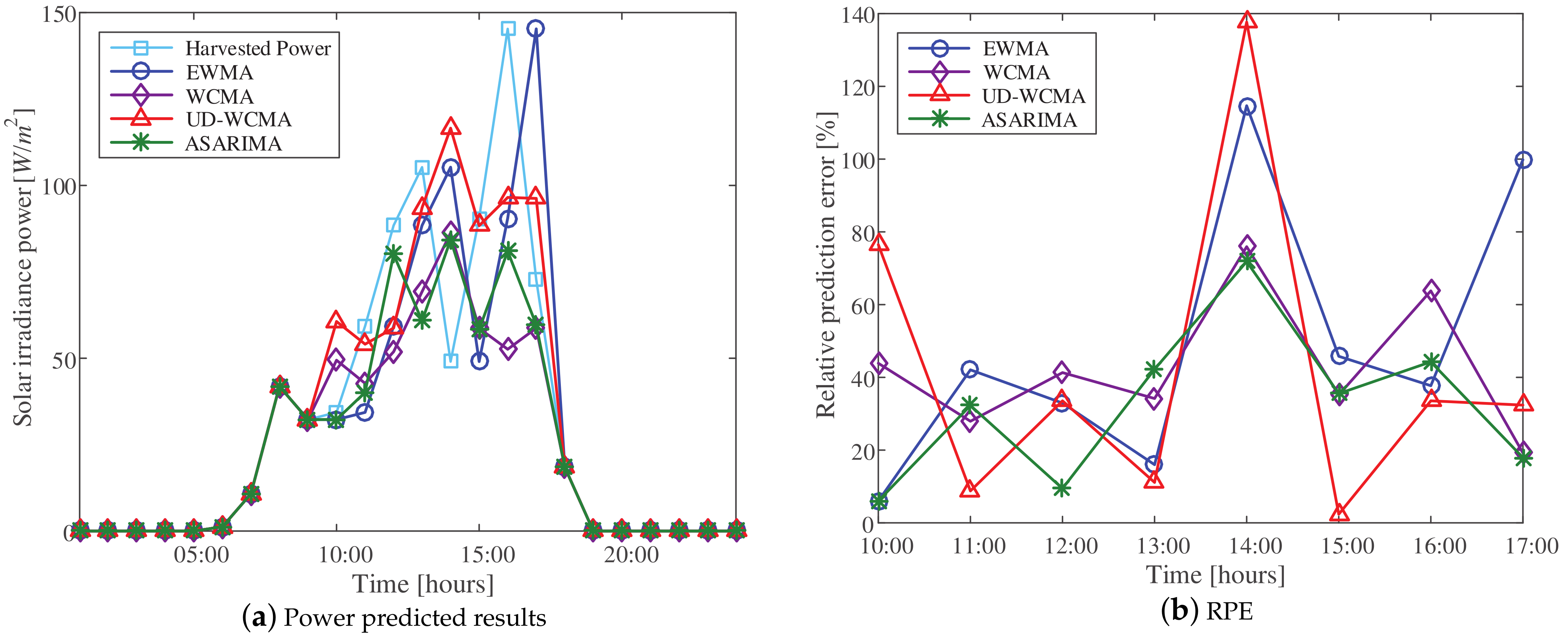
5.2. Comparing the Relative Errors of Different Schemes

In the following section, we compare the ASARIMA with other existing prediction algorithms, i.e., the EWMA, WCMA, and UD-WCMA. A weighting factor $\alpha$ exists in the EWMA and WCMA algorithms, and this weighting factor affects the prediction accuracy. However, the ASARIMA proposed in this paper does not have the limitations of the abovementioned two algorithms. To analyze the effect of the proposed prediction scheme, we select an optimal ASARIMA for the daily prediction of the EWMA and WCMA algorithms to optimize the EWMA and WCMA forecasting results. The relative errors of each algorithm are exhibited in Figure 5.

In Figure 5, among the abovementioned algorithms, the prediction effect of the ASARIMA has evident advantages. In particular, the proposed algorithm has an advantage over the other algorithms under stable weather conditions. For example, on April 13, the relative error of the EWMA algorithm is 24.56%, those of the WCMA and UD-WCMA algorithms are close to 10%, and that of the proposed algorithm is less than 3%. In comparison with the prediction efficiency of the EWMA algorithm, that of the proposed ASARIMA model improved by at least 70%.

Figure 6, Figure 7 and Figure 8 are solar harvested power predicted results and relative prediction errors (RPE) for the different weather conditions of April 14, April 15, and April 17, respectively. The relative error of the proposed ASARIMA can also be improved despite the unstable weather conditions. For example, on April 15, the relative error of the EWMA algorithm is 49.39%, those of the WCMA and UD-WCMA algorithms are close to 42%, and that of the ASARIMA model is only 32.45%. The relative prediction efficiency of the ASARIMA algorithm is also improved by 22.7%. We present the forecast trend chart of the ASARIMA algorithm in the following days and the relative error of each prediction time for a specific analysis, as illustrated in Figure 6.

When weather conditions are continuous and stable, as demonstrated in Figure 6a, a comparison of the four prediction methods reflects that the relative error of the ASARIMA model at each prediction moment is at the minimum value, which indicates that the prediction of the ASARIMA model is close to the actual situation. At this point, the EWMA algorithm appears dented when it approaches the highest point, thus leading to a large error. Simultaneously, the UD-WCMA and WCMA have poor adaptability, as reflected in the hysteresis of the highest point of the prediction, and the maximum value of the prediction is greater than the actual value.

When rain or sunshine is variable under weather conditions, as exhibited in Figure 7, the weather conditions before a certain day were partly sunny and partly cloudy, thus making the prediction difficult. Given the influence of hysteresis, the result of the EWMA’s prediction is one beat slower, that is, we have the illusion that the corresponding point moves backward. Model matching of the UD-WCMA is difficult to realize, which leads to a large deviation in the prediction results. The WCMA’s prediction at 16:00 reflects a large deviation. The algorithm proposed in this paper constantly fluctuates around a certain value, and the prediction shows a slightly larger deviation at individual points but is relatively stable overall.

When the weather conditions change from the previous high volatility to stable, as presented in Figure 8, the WCMA and UD-WCMA algorithms still demonstrate strong volatility interference in the prediction trend due to the influences of previous weather conditions; consequently, the prediction effect is not equally as favorable as that of the new algorithm. The proposed ASARIMA algorithm has good adaptability when weather conditions change significantly or remain stable.

From January 2018 to December 2018, the comparison of the monthly mean relative prediction error of the EWMA, WCMA, Pro-Energy, ARIMA, and ASARIMA algorithms is shown in Figure 9. It can be seen from Figure 9 that the prediction algorithm ASARIMA proposed in this paper has advantages over other algorithms in terms of monthly mean relative prediction error.

6. Conclusions

Solar power generation is affected by climatic factors, such as sunshine, seasonal changes, and weather fluctuations. These cause discontinuity, periodicity, and uncertainty in the output power of the power generation system. In this paper, we use the Euclidean distance to measure the weather similarity and optimize the training set of the SARIMA model. We adjust the order of the data adaptively in accordance with the similarity between the data of the current day and several reference days. When the reference day is similar to the current day, it is considered close to the current day. The prediction can adapt not only to similar continuous weather conditions but also to the evident change in weather conditions. The accuracy of prediction is significantly improved, and the ASARIMA model has advantages over other models.

References

1. Akyildiz, I.F.; Vuran, M.C. Wireless Sensor Networks; John Wiley & Sons, Inc.: New York, NY, USA, 2010. [Google Scholar]
2. Zhou, J.; Han, T.; Xiao, F.; Gui, G.; Adebisi, B.; Gacanin, H.; Sari, H. Multi-scale network traffic prediction method based on deep echo state network for internet of things. IEEE Internet Things J. 2022. [Google Scholar] [CrossRef]
3. Adu-Manu, K.S.; Adam, N.; Tapparello, C.; Ayatollahi, H.; Heinzelman, W. Energy-Harvesting Wireless Sensor Networks (EH-WSNs): A Review. ACM Trans. Sens. Netw. 2018, 14, 2. [Google Scholar] [CrossRef]
4. Du, X.; Li, Y.; Zhou, S.; Zhou, Y. ATS-LIA: A lightweight mutual authentication based on adaptive trust strategy in flying ad-hoc networks. Peer-to-Peer Netw. Appl. 2022, 15, 1979–1993. [Google Scholar] [CrossRef] [PubMed]
5. Engmann, F.; Katsriku, F.A.; Abdulai, J.D.; Adu-Manu, K.S.; Banaseka, F.K. Prolonging the lifetime of wireless sensor networks: A review of current techniques. Wirel. Commun. Mob. Comput. 2018. [Google Scholar] [CrossRef]
6. Ashraf, N.; Faizan, M.; Asif, W.; Qureshi, H.K.; Iqbal, A.; Lestas, M. Energy management in harvesting enabled sensing nodes: Prediction and control. J. Netw. Comput. Appl. 2019, 132, 104–117. [Google Scholar] [CrossRef]
7. Kansal, A.; Hsu, J.; Zahedi, S.; Srivastava, M.B. Power management in energy harvesting sensor networks. ACM Trans. Embed. Comput. Syst. 2007, 6, 32es. [Google Scholar] [CrossRef]
8. Introduction of ARIMA. Available online: http://people.duke.edu/~rnau/411arim.htm (accessed on 20 May 2022).
9. Cavanaugh, J.E.; Neath, A.A. The Akaike information criterion: Background, derivation, properties, application, interpretation, and refinements. Wiley Interdiscip. Rev. Comput. Stat. 2019, 11, E1460. [Google Scholar] [CrossRef]
10. Ding, M.; Wang, L.; Bi, R. An ANN-based Approach for Forecasting the Power Output of Photovoltaic System. Procedia Environ. Sci. 2011, 11, 1308–1315. [Google Scholar] [CrossRef]
11. Liu, Q.; Zhang, Q. Accuracy improvement of energy prediction for solar-energy-powered embedded systems. IEEE Trans. Very Large Scale Integr. (VLSI) Syst. 2016, 24, 2062–2074. [Google Scholar] [CrossRef]
12. Asrari, A.; Wu, T.X.; Ramos, B. A Hybrid Algorithm for Short-Term Solar Power Prediction-Sunshine State Case Study. IEEE Trans. Sustain. Energy 2017, 8, 582–591. [Google Scholar] [CrossRef]
13. Recas Piorno, J.; Bergonzini, C.; Atienza, D.; Rosing, T.S. Prediction and management in energy harvested wireless sensor nodes. In Proceedings of the 2009 1st International Conference on Wireless Communication, Vehicular Technology, Information Theory and Aerospace & Electronic Systems Technology, Aalborg, Denmark, 17–20 May 2009; pp. 6–10. [Google Scholar]
14. Cammarano, A.; Petrioli, C.; Spenza, D. Pro-energy: A novel energy prediction model for solar and wind energy-harvesting wireless sensor networks. In Proceedings of the 2012 IEEE 9th International Conference on Mobile Ad-Hoc and Sensor Systems (MASS 2012), Las Vegas, NV, USA, 8–11 October 2012; pp. 75–83. [Google Scholar]
15. Cammarano, A.; Petrioli, C.; Spenza, D. Online energy harvesting prediction in environmentally powered wireless sensor networks. IEEE Sens. J. 2016, 16, 6793–6804. [Google Scholar] [CrossRef]
16. Dehwah, A.H.; Elmetennani, S.; Claudel, C. Ud-WCMA: An energy estimation and forecast scheme for solar powered wireless sensor networks. J. Netw. Comput. Appl. 2017, 90, 17–25. [Google Scholar] [CrossRef]
17. Long, H.; Zhang, C.; Geng, R.; Wu, Z.; Gu, W. A Combination Interval Prediction Model based on Biased Convex Cost Function and Auto Encoder. IEEE Trans. Sustain. Energy 2021, 12, 1561–1570. [Google Scholar] [CrossRef]
18. Ye, X. The application of ARIMA model in chinese mobile user prediction. In Proceedings of the 2010 IEEE International Conference on Granular Computing, San Jose, CA, USA, 14–16 August 2010; pp. 586–591. [Google Scholar]
19. Ma, W.; Pang, Y.; Zou, J. The application of ARIMA in short-timely forecasting for motion of planning boat. In Proceedings of the 2011 International Conference on Computer Science and Service System (CSSS), Nanjing, China, 27–29 June 2011; pp. 3651–3654. [Google Scholar]
20. Li, Q.; Guo, N.-N.; Han, Z.Y.; Zhang, Y.B.; Qi, S.X.; Xu, Y.G.; Wei, Y.-M.; Han, X.; Liu, Y.Y. Application of an autoregressive integrated moving average model for predicting the incidence of hemorrhagic fever with renal syndrome. AM J. Trop. Med. Hyg. 2012, 87, 364–370. [Google Scholar] [CrossRef] [PubMed]
21. Juang, W.C.; Huang, S.J.; Huang, F.D.; Cheng, P.W.; Wann, S.R. Application of time series analysis in modelling and forecasting emergency department visits in a medical centre in southern taiwan. BMJ Open 2017, 7, e018628. [Google Scholar] [CrossRef] [PubMed]
22. Etuk, E.H.; Ojekudo, N. Another look at the SARIMA modelling of the number of dengue cases in campinas, State of Sao Paulo, Brazil. Int. J. Nat. Sci. Res. 2014, 2, 156–164. [Google Scholar]
23. Elganainy, M.; Eldwer, A.E. Stochastic forecasting models of the monthly streamflow for the blue nile at eldiem station. Water Resour. 2018, 45, 326–337. [Google Scholar] [CrossRef]
24. Maxey, C.; Andreas, A. Oak Ridge National Laboratory (ORNL); Rotating Shadowband Radiometer (RSR); Oak Ridge, Tennessee (Data); NREL Report No. DA-5500-56512; National Renewable Energy Lab. (NREL): Golden, CO, USA, 2007. [Google Scholar] [CrossRef]
25. Liu, S.; Kong, X.; Xie, A.; Shen, Y.; Zhu, J.; Li, C.; Zhang, Q. A study of the fractal structure of the precipitate and the mechanism of its formation from the gallbladder bile of a patient. Russ. J. Phys. Chem. A 2007, 81, 2084–2089. [Google Scholar] [CrossRef]
26. Benjamin, M.A.; Rigby, R.A.; Stasinopoulos, D.M. Generalized autoregressive moving average models. J. Am. Stat. Assoc. 2003, 98, 214–223. [Google Scholar] [CrossRef]
Figure 1. The flow chart of ASARIMA model.
Electronics 11 02934 g001
Figure 2. Solar irradiance power from 13 to 18 April 2018.
Electronics 11 02934 g002
Figure 3. The ACF/PACF chart of time series.
Electronics 11 02934 g003
Figure 4. Three time-series model prediction results of 17 April 2018.
Electronics 11 02934 g004
Figure 5. The relative errors of various algorithms
Electronics 11 02934 g005
Figure 6. Power predicted and prediction error for 14 April 2018.
Electronics 11 02934 g006
Figure 7. Power predicted and prediction error for 15 April 2018.
Electronics 11 02934 g007
Figure 8. Power predicted and prediction error for 17 April 2018.
Electronics 11 02934 g008
Figure 9. Comparison of the monthly mean relative prediction error of five algorithms on January 2018 to Dececember 2018.
Electronics 11 02934 g009