1. Introduction
As of 2020, China’s car ownership exceeds 280 million, and the huge car ownership has created great development space for the used car market. At the same time, with the implementation of China VI (the national sixth phase of motor vehicle pollutant emission standards is to implement the relevant laws and control the environmental pollution of compression-ignited and gas-fuel ignited engine vehicle exhaust) and the current widespread popularity of electric vehicles, the value of the retention rate of newly purchased cars is low, and many of the cars currently flowing in the market will be processed, which will lead to the accelerated development of the used car market.
In the context of the era of big data, people’s lives are slowly being digitized and Internetized. The Internet turns most commodity transactions into e-commerce; that is, many transactions can be carried out on the Internet, such as Taobao, JD, Pinduoduo and many other e-commerce platforms, making people’s lives more convenient. Similarly, the Internet has also turned used car trading into e-commerce, such as 58.com and other used car trading platforms. The e-commerce of used car transactions has further pushed the used car market to a climax, and various problems have gradually emerged, such as the lack of a unified standard for judging the value of used car assets. Used cars are affected not only by the basic configuration of the body—brand, car system and power—but also by the condition, mileage and age of the car, resulting in differences between the prices of used cars—one car, one condition and one price. Therefore, how to effectively assess the price of used cars requires a scientific valuation conversion method.
With the rapid development of machine learning methods and deep learning methods, it is possible to automate price prediction. Zhang et al. [
1] introduced a complete integrated empirical modal decomposition algorithm with adaptive noise to extract the characteristics of stock price time series on the time scale and combined the attention mechanism with the neural network of the gated recurrent unit to predict stock prices and the Shanghai composite index. Cao et al. [
2] designed an online short-term rental market price prediction model based on XGBoost and introduced a SHAP model to explain the characteristics. Fathalla et al. [
3] proposed using a deep neural network based on LSTM and convoluted neural networks to predict price prediction, and the proposed model achieved a better average absolute error accuracy score than SVM. Based on the regression algorithm of random forest, Yan et al. [
4] combined the Pearson coefficient and an improved grid search method to predict stock prices. Yao et al. [
5] used HP filtering to decompose the stock index price time series into long-term trends and short-term fluctuations, used the LSTM neural network model to learn its sequence characteristics and make predictions, and fused the prediction results to obtain the stock index price prediction results. Kky et al. [
6] proposed a hybrid GA-XGBoost prediction system with an enhanced feature engineering process consisting of feature set expansion, data preparation, and optimal feature set selection using the hybrid GA-XGBoost algorithm. Le et al. [
7] propose to apply k-means, a clustering technique, together with Gradient Boost and XGBoost models to improve the prediction performance. Hernández-Casas et al. [
8] successfully used an artificial neural network model to predict Mexican lobster export prices. Xu et al. [
9] found that the displacement-prediction effect of XGBoost algorithm is better than that of SVR and RNNs in the sliding process of landslide with a large displacement value and small numbers of samples.
The used car market can be traced back to the beginning of the last century. After decades of development, the ratio of new cars to used cars has reached 1:3, and such a rapid development rate has caused a wave of research on the price of used cars by scholars in various fields. Purohit [
10] studied the correlation between the used car market and the new car market and found that the price of used cars decreases as the number of new cars increases, and its consumers are more inclined to buy models with slow depreciation. Hansen et al. [
11] developed a statistical model for the resale price prediction of used cars and found that random forests were more appropriate through empirical studies. Hu et al. [
12] proposed the replacement cost method, which evaluates the price of the car on the basis of the classification treatment of the vehicle, but because the method is based on the price of the new car and there are many uncertain factors in the automobile market, there is uncertainty about the effect of the model. Andrews et al. [
13] analyzed the relevant information of the eBay used car auction market through a linear regression method and concluded that car property rights and auction duration have a greater impact on price. To study the impact of the characteristics of the used car on the price, Richardson [
14] analyzed multiple characteristics through a multiple regression analysis and concluded that the hybrid vehicle is more valuable. Qiang et al. [
15] believed that when using the traditional methods to process massive data, there would be problems such as a slow processing speed and low accuracy, so they proposed a comprehensive optimization method based on the combination of a BP neural network and nonlinear curve fitting; the nonlinear curve fitting was carried out on the output of the BP neural network model, which greatly improved the accuracy of the price prediction of used cars. Zhang [
16] established a multiple linear regression model and an artificial neural network model based on the crawled data of nearly 5000 used cars and found that the prediction accuracy of the artificial neural network model was higher by comparison. Liu [
17] proposed predicting the price with the help of artificial neural networks without considering the vehicle condition, and then combining the prediction results with the vehicle condition factors to make a secondary prediction of the price, which obtained good results.
To further improve the accuracy of used car price prediction and improve the accuracy of existing mainstream models, this paper proposes an iterative framework of XGBoost+LightGBM. First, by training the deep residual network model, the training results are fused with the original features as new features. The resulting features are then repeatedly trained in the iterative framework to improve the prediction accuracy of the model. Finally, the effect of the model framework is verified by experiments, and the universality of the framework is verified by combining it with a variety of existing mainstream methods.
2. Models and Methods
2.1. Deep Residual Network
ResNet (deep residual network) is a network model that has been improved based on a deep convolutional neural network [
18], and by learning the development process of a deep convolutional neural network, it can be found that the expression ability of the network increases with increasing the network depth. He Kaiming et al. [
19,
20,
21] proved through experiments that for two network structures with the same time complexity, the deeper the structure, the better the performance. However, as the number of network layers increases to a certain extent, the network’s performance degrades significantly. To solve this problem, a deep residual learning network is proposed.
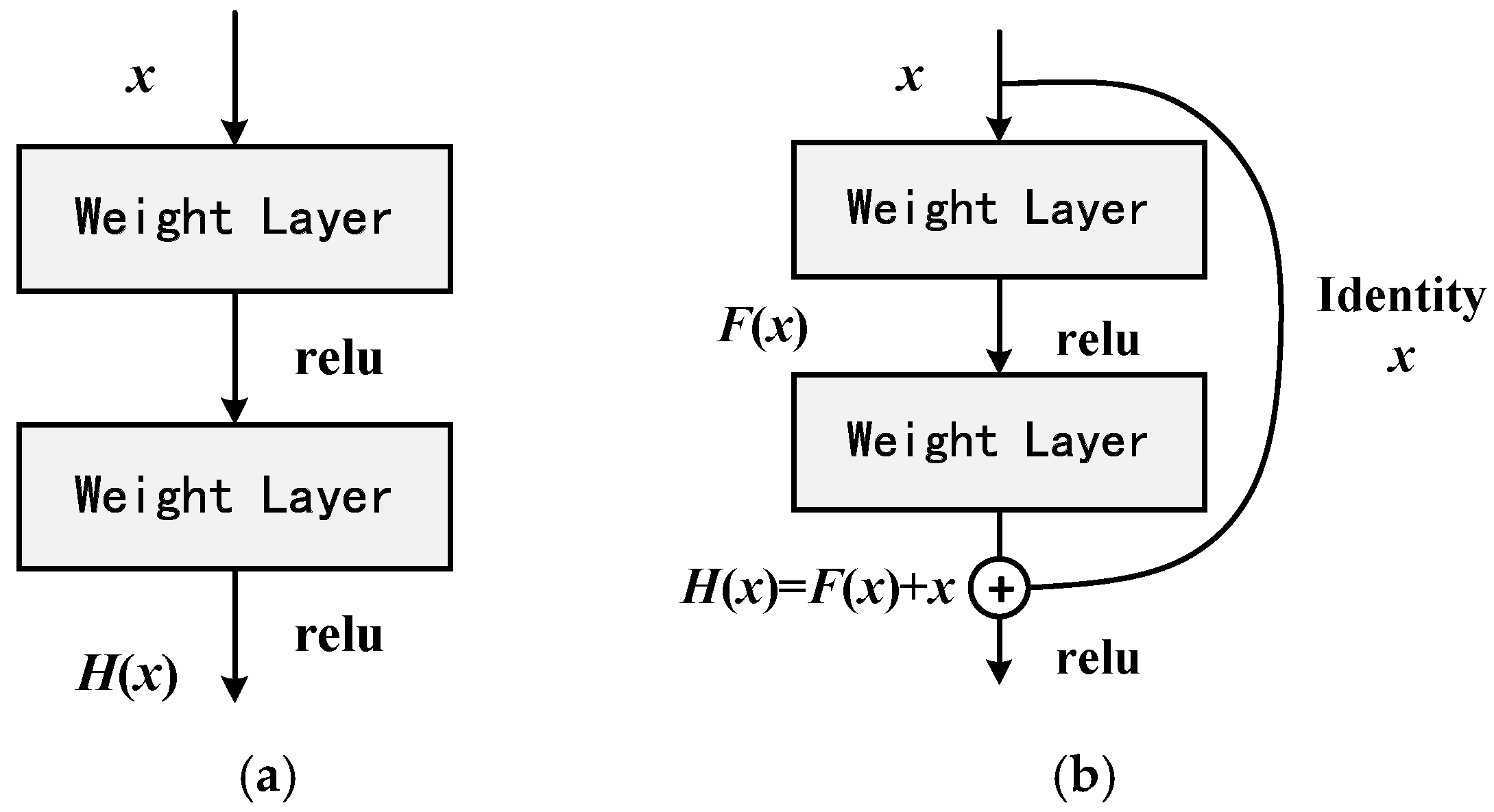
Figure 1 shows a schematic diagram of the residual unit of the residual network. It can be seen from the figure that the output of the residual unit is obtained by adding the output of multiple convolutional layers and the original input, and then activated by the ReLU function, and the residual network is obtained by multiple residual units.
For a residual unit, there is a functional relationship, as follows:
where
is the output of the lth residual unit and
is the input of the lth residual unit.
Let
, then we have
That is, the input of the Lth residual unit can be expressed as the input of a residual unit of a certain layer and the sum of all the complex maps in the middle of it. If ε denotes the loss function, then by calculation, the backpropagation is calculated:
Obviously, at this time, the successive multiplication disappears, that is, the vanishing gradient will not exist.
The precondition of the above analysis is ; to achieve this effect, the residual structure must be reconstructed. The improved residual structure fuses the activation layer into the residual branch and uses the residual unit preactivated by ReLU to satisfy the preconditions of the above analysis.
2.2. XGBoost
The XGBoost model [
22] is a tree-based gradient boosting integrated model that is actually composed of multiple classification regression trees (CART) that learn the residual value of the sum of the target value and the predicted values of all previous decision trees, make a common decision after all decision trees have completed training, and finally accumulate the samples in the previous prediction results as the final prediction result.
During the XGBoost model training phase, each new tree is trained based on the tree that has been trained, and when a decision tree is generated, it needs to be pruned to prevent overfitting. To reduce the error, the XGBoost model trains the error obtained by each tree as the input of the next tree for training again, and gradually reduces the prediction error so that the model prediction result is gradually forced to the true value.
Suppose that (
) is the sample used in training. Then, the XGBoost prediction model can be expressed as
where
,
,
x represents the eigenvector,
y represents the sample label, and
represents the
kth decision tree.
The corresponding objective function is defined as follows:
The objective function
Obj(0) consists of two parts: the first part is the loss function determined by the specific task to assess the accuracy of the model’s predictions; the second part is the regularization term, which is used to reduce the possibility of overfitting linearity in the model; The function is as follows:
where
γ is the leaf node coefficient, and the function is to make XGBoost optimize and adjust the objective function, which is equivalent to a pre-pruning operation (that is,
γT controls the complexity of the tree, and the larger the value, the greater the objective function value, which then suppresses the complexity of the model). While
λ is the coefficient of the squared mode of
L2, it also suppresses overfitting, and the entire
L2 regularization term is used to control the leaf node weight fraction. If the value of the regularization term is 0, then the objective function is GBDT.
The XGBoost model adds regularization terms to the objective function and reduces the possibility of overfitting. It uses not only the first derivative, but also the second derivative to increase the accuracy of the loss function and customize the loss.
2.3. LightGBM
LightGBM [
23] is a high-speed, distributed, and high-performance gradient boosting framework; its full name is Lightweight Efficient Gradient Boosting Tree (LGBM). It is based on a decision tree algorithm that can be used to complete sorting, classification, regression, and many other machine learning tasks. Under the condition of not reducing the accuracy, the speed is increased by approximately ten times, and the memory occupied is reduced by approximately three times, which has the advantages of high training efficiency, low memory occupation, high precision, and support for parallelism, and GPU can be used to process large-scale data. The main technical details of LGBM are as follows [
24]:
LightGBM is a decision tree algorithm based on histograms, which has great advantages in memory consumption and computational cost. The principle is as follows: first, discretize the continuous floating-point eigenvalues, convert them to k integers, and construct them as a histogram (bins) with a width value equal to k. When traversing the data, the discretized value is used as an index, and the statistics are accumulated in the histogram. After a data traversal, the required statistic has been accumulated in the histogram and then iterated in conjunction with the index of the histogram to search for the best partition point. Therefore, when performing node splitting, it is not necessary to calculate all the data when traversing each feature, but only k times, and the complexity is optimized from O(data * feature) to O(k* feature), which greatly accelerates the speed of training.
- (2)
Leafwise
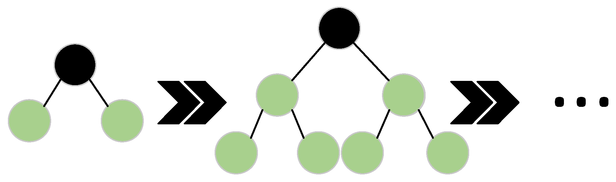
The traditional GBDT algorithm splits each node of each larger node in parallel at the same time as the decision tree. This growth method is called levelwise growth, as shown in
Figure 2, which treats each leaf of the same layer equally. However, some leaves in normal training do not need to continue to split and search, resulting in a waste of resources and excessive time expenditure.
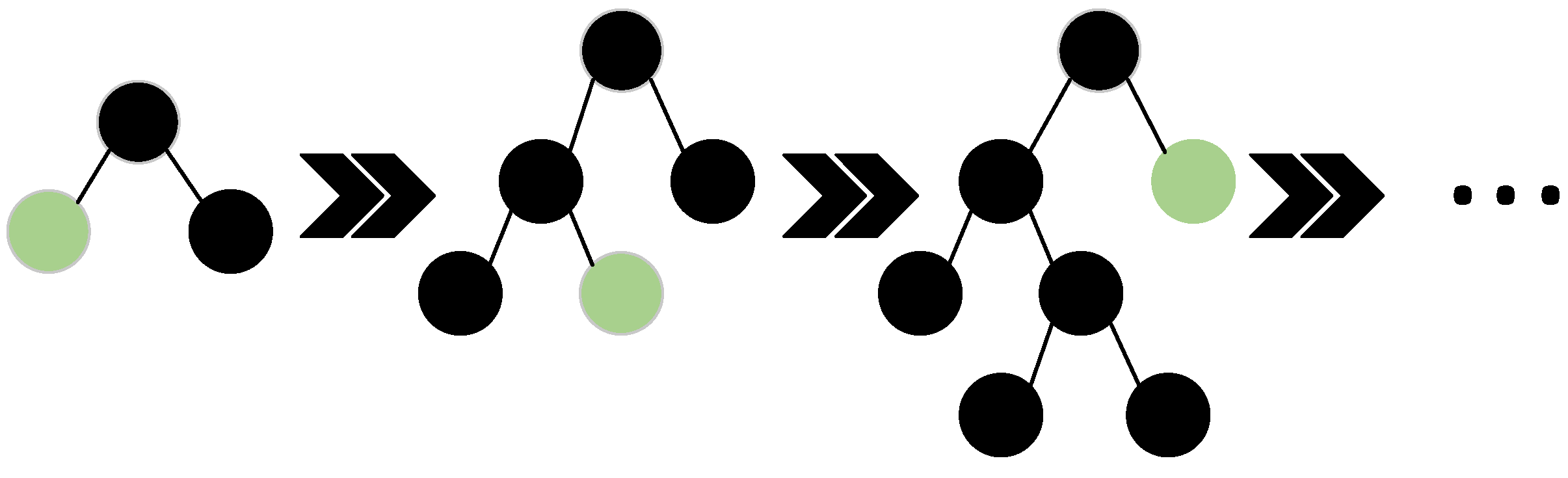
Therefore, LGBM proposes a more efficient strategy of leafwise growth. This method selects only the leaves with the largest splitting gain when splitting each layer of leaves, which can effectively reduce the time expenditure, as shown in
Figure 3.
- (3)
Histogram Error Acceleration
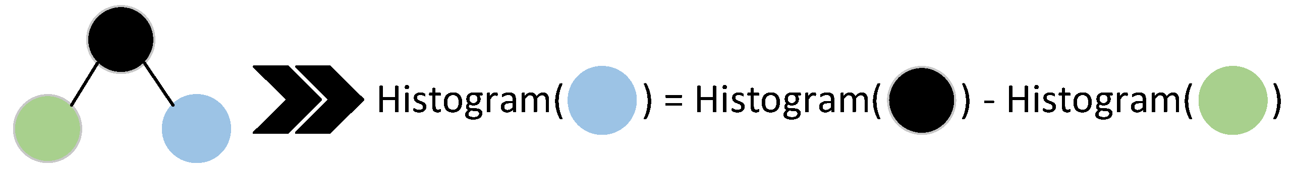
Generally, as shown in
Figure 4, after the black node splits into green child nodes, the histogram of the blue node can be obtained directly from the black node minus the green node, which greatly reduces the time overhead.
- (4)
Gradient-Based One-Sided Sampling (GOSS)
LGBM is trained based on gradients, where the GBDT algorithm inputs all samples into the next classifier for training, but the optimization of the loss function is determined by those sample points with very large gradients, so LGBM uses the GOSS method to retain all large gradient samples and randomly selects some small gradient samples proportionally to participate in subsequent training. If there are 1 million pieces of data, of which 50,000 are large gradient samples (the gradient size threshold can be determined by yourself) and the rest are small gradient samples, the algorithm keeps these 50,000 samples and then randomly takes x% (x is a hyperparameter) samples from the small gradient sample size, which can also improve the speed.
2.4. DXL Model
To further improve the performance of the price prediction model, this paper com-bines the machine learning model and the deep learning model to design an XGB+LGBM iterative framework for multiple models. In this paper, a combination of ResNet and iterative framework is chosen to verify the performance of the XGB+LGBM iterative framework, and the combined model is named DXL (Deep Residual Network-XGB+LGBM).
Whether it is a machine learning model or a deep learning model, the downstream task is completed by learning the characteristics of the data. Then, we determine whether the repeated training will obtain better results by combining the obtained results as new features with the original features into a group of new features.
As an important step in the development of artificial intelligence, the effect of neural networks has been widely recognized by scholars in various fields, but it is limited by the size of the data scale, and overlarge-scale data will also reduce the training speed, so it is not suitable for iterative loops. However, XGBoost and LightGBM have been widely used in a variety of prediction tasks in recent years, and both are extension algorithms based on decision trees, which assume that they have the same sensitivity to the same features. Multimodel alternate iterative training also avoids the excessive dependence of a single model iterative learning on new features.
Through the above analysis, the XGBoost and LightGBM models are combined to obtain the XGB+LGBM iterative framework, and the new features are used for iterative learning training.
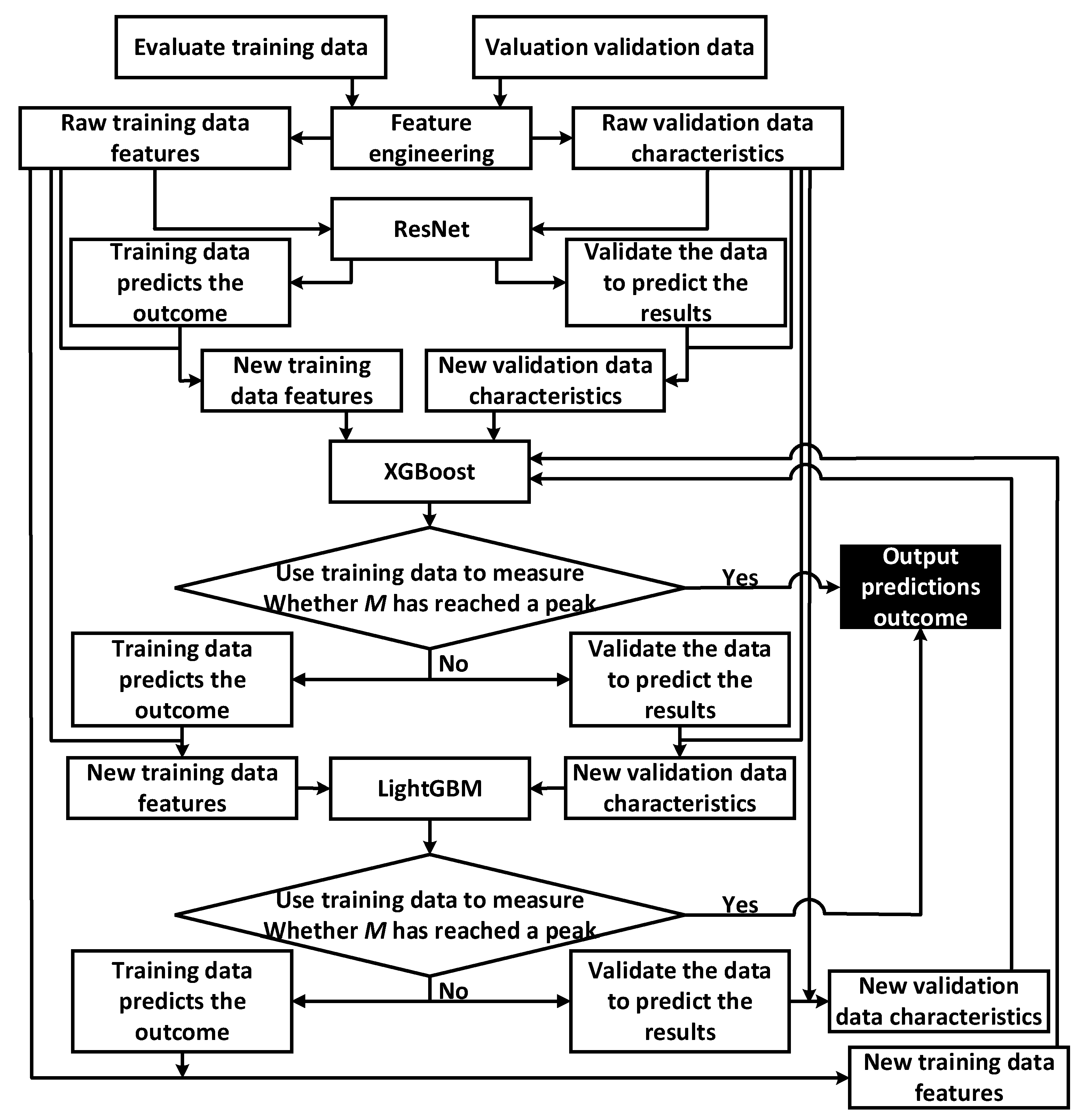
Figure 5 is the flowchart of the DXL model, and the specific steps of the model are as follows:
Step 1: The original data are preprocessed and feature engineered to obtain the original features.
Step 2: The original feature is trained into the deep residual network, and the result is combined with the original feature to form a new set of features.
Step 3: Input the new features into XGBoost for training, evaluate the results, and output the results if the peak is reached; otherwise, combine the results as new features with the original features to form a new set of features.
Step 4: Input the new features into LightGBM for training, evaluate the results, and output the results if the peak is reached; otherwise, combine the results as new features with the original features to obtain a new set of features, and then complete Step 3.
The DXL Algorithm 1 pseudocode is as follows:
| Algorithm 1: DXL algorithm |
Input: Train_data and Test_data (No label);
Output: Prediction results Pr of Test_data;
Training ResNet models by using Train_data;
The results of Train_data and Test_data predicted by using the trained ResNet model;
Add the prediction result as a new feature pre_result to the original feature;
min_loss = ∞;
index = 1;
while loss < min_loss do:
min_loss = loss;
if index%2 == 1:
Training with XGB;
else:
Training with LGBM;
Calculate the average loss value between the predicted and actual values of Train_data;
The pre_result feature is replaced with the current round prediction Pr;
end
Output prediction results Pr; |
4. Conclusions
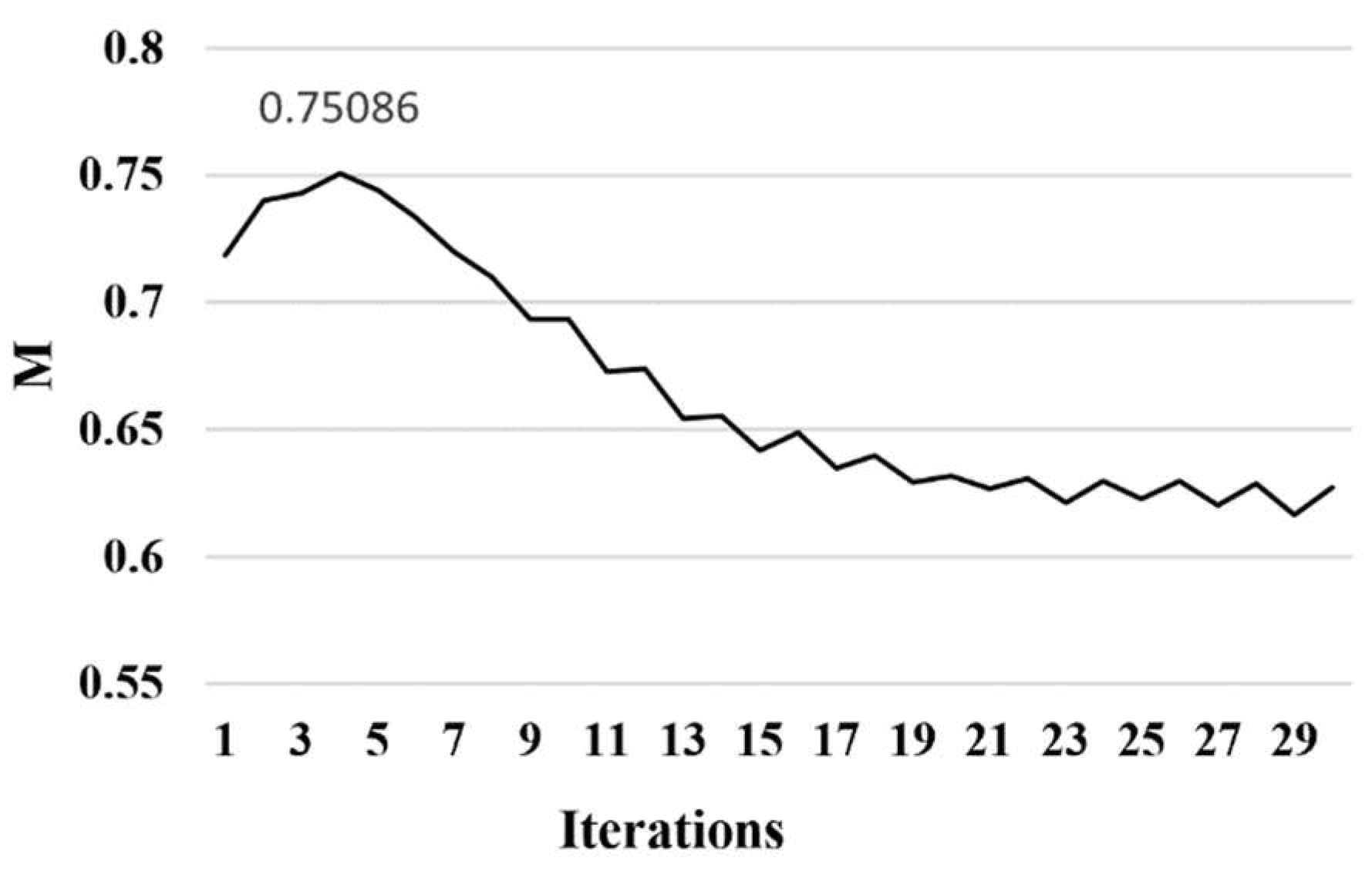
With the rapid growth of the economy, the car ownership rate is rising, which also bestows the used car market with excellent development prospects, but the accuracy of existing models in the price prediction task is average. Taking the real car data provided by the MathorCup big data competition as the research object, this paper constructs a model framework based on multimodel fusion. First, by training the deep residual network, the prediction results are fused with the original features as new features. Second, the combined features are input into the XGB+LGBM iterative framework, and the prediction results are output when the M index reaches its peak through cross-validation. Then, the effectiveness of the DXL algorithm is verified by comparative experiments with five mainstream algorithms: linear regression, random forest, XGB, LGBM and depth residual network. Finally, by combining the four mainstream algorithms with the XGB+LGBM iterative framework, it is verified that the XGB+LGBM iteration framework can be applied to other models and greatly improve the performance of the original model.


