An Improved Hierarchical Clustering Algorithm Based on the Idea of Population Reproduction and Fusion

Abstract

Aiming to resolve the problems of the traditional hierarchical clustering algorithm that cannot find clusters with uneven density, requires a large amount of calculation, and has low efficiency, this paper proposes an improved hierarchical clustering algorithm (referred to as PRI-MFC) based on the idea of population reproduction and fusion. It is divided into two stages: fuzzy pre-clustering and Jaccard fusion clustering. In the fuzzy pre-clustering stage, it determines the center point, uses the product of the neighborhood radius eps and the dispersion degree fog as the benchmark to divide the data, uses the Euclidean distance to determine the similarity of the two data points, and uses the membership grade to record the information of the common points in each cluster. In the Jaccard fusion clustering stage, the clusters with common points are the clusters to be fused, and the clusters whose Jaccard similarity coefficient between the clusters to be fused is greater than the fusion parameter jac are fused. The common points of the clusters whose Jaccard similarity coefficient between clusters is less than the fusion parameter jac are divided into the cluster with the largest membership grade. A variety of experiments are designed from multiple perspectives on artificial datasets and real datasets to demonstrate the superiority of the PRI-MFC algorithm in terms of clustering effect, clustering quality, and time consumption. Experiments are carried out on Chinese household financial survey data, and the clustering results that conform to the actual situation of Chinese households are obtained, which shows the practicability of this algorithm.

1. Introduction

Clustering [1] is a process of dividing a set of data objects into multiple groups or clusters, so that objects in a cluster have high similarity, but it is very dissimilar to objects in other clusters [2,3,4,5]. It is also an unsupervised machine learning technique that does not require labels associated with data points [6,7,8,9,10]. As a data mining and machine learning tool, clustering has been rooted in many application fields, such as pattern recognition, image analysis, statistical analysis, business intelligence, and other fields [11,12,13,14,15]. In addition, the feature selection methods are also proposed to deal with data [16].

The basic idea of the hierarchical clustering algorithm [17] is to construct the hierarchical relationship between data for clustering. The obtained clustering result has the characteristics of a tree structure, which is called a clustering tree. It is mainly performed using two methods, agglomeration techniques such as AGNE (agglomeration analysis) and divisive techniques such as DIANA (division analysis) [18]. Regardless of agglomeration technology or splitting technology, a core problem is measuring the distance between two clusters, and time is basically spent on distance calculation. Therefore, a large number of improved algorithms that use different means to reduce the number of distance calculations have been proposed one after another to improve algorithmic efficiency [19,20,21,22,23,24,25,26,27]. Guha et al. [28] proposed the CURE algorithm, which considers sampling the data in the cluster and uses the sampled data as representative of the cluster to reduce the amount of calculation of pairwise distances. The Guha team [29] improved CURE and proposed the ROCK algorithm, which can handle non-standard metric data (non-Euclidean space, graph structure, etc.). Karypis et al. [30] proposed the Chameleon algorithm, which uses the K-nearest-neighbor method to divide the data points into many small cluster sub-clusters in a two-step clustering manner before hierarchical aggregation in order to reduce the number of iterations for hierarchical aggregation. Gagolewski et al. [31] proposed the Genie algorithm which calculates the Gini index of the current cluster division before calculating the distance between clusters. If the Gini index exceeds the threshold, the merging of the smallest clusters is given priority to reduce pairwise distance calculation. Another hierarchical clustering idea is to incrementally calculate and update the data nodes and clustering features (abbreviated CF) of clusters to construct a CF clustering tree. The earliest proposed CF tree algorithm BIRCH [32] is a linear complexity algorithm. When a node is added, the number of CF nodes compared does not exceed the height of the clustering tree. While having excellent algorithm complexity, the BIRCH algorithm cannot ensure the accuracy and robustness of the clustering results, and it is extremely sensitive to the input order of the data. Kobren et al. [33] improved this and proposed the PERCH algorithm. This algorithm adds two optimization operations which are the rotation of the binary tree branch and the balance of the tree height. This greatly reduces the sensitivity of the data input order. Based on the PERCH algorithm, the PKobren team proposed the GRINCH algorithm [34] to build a single binary clustering tree. The GRINCH algorithm adds the grafting operation of two branches, allowing the ability to reconstruct, which further reduces the algorithm sensitivity to the order of data input, but, at the same time, it greatly reduces the scalability of the algorithm. Although most CF tree-like algorithms have excellent scalability, their clustering accuracy on real-world datasets is generally lower than that of classical hierarchical aggregation clustering algorithms.

To discover clusters of arbitrary shapes, density-based clustering algorithms are born. Ester et al. [35] proposed a DBSCAN algorithm based on high-density connected regions. This algorithm has two key parameters, Eps and Minpts. Many scholars at home and abroad have studied and improved the DBSCAN algorithm for the selection of Eps and Minpts. The VDBSCAN algorithm [36] selects the parameter values under different densities through the K-dist graph and uses these parameter values to cluster clusters of different densities to finally find clusters of different densities. The AF-DBSCAN algorithm [37] is an algorithm for adaptive parameter selection, which adaptively calculates the optimal global parameters Eps and MinPts according to the KNN distribution and mathematical statistical analysis. The KANN-DBSCAN algorithm [38] is based on the parameter optimization strategy and automatically determines the Eps and Minpts parameters by automatically finding the change and stable interval of the cluster number of the clustering results to achieve a high-accuracy clustering process. The KLS-DBSCAN algorithm [39] uses kernel density estimation and the mathematical expectation method to determine the parameter range according to the data distribution characteristics. The reasonable number of clusters in the data set is calculated by analyzing the local density characteristics, and it uses the silhouette coefficient to determine the optimal Eps and MinPts parameters. The MAD-DBSCAN algorithm [40] uses the self-distribution characteristics of the denoised attenuated datasets to generate a list of candidate Eps and MinPts parameters. It selects the corresponding Eps and MinPts as the initial density threshold according to the denoising level in the interval where the number of clusters tends to be stable.

To represent the uncertainty present in the data, Zadeh [41] proposed the concept of fuzzy sets, which allow elements to contain rank membership values from the interval [0, 1]. Correspondingly, the widely used fuzzy C-means clustering algorithm [42] is proposed, and many variants have appeared since then. However, membership levels alone are not sufficient to deal with the uncertainty that exists in the data. With the introduction of the hesitation class by Atanassov, Intuitive Fuzzy Sets (IFS) [43] emerge, in which a pair of membership and non-membership values for an element is used to represent the uncertainty present in the data. Due to its better uncertainty management capability, IFS is used in various clustering techniques, such as Intuitionistic Fuzzy C-means (IFCM) [44], improved IFCM [45], probabilistic intuitionistic fuzzy C-means [46,47], Intuitive Fuzzy Hierarchical Clustering (IFHC) [48], and Generalized Fuzzy Hierarchical Clustering (GHFHC) [49].

Most clustering algorithms assign each data object to one of several clusters, and such cluster assignment rules are necessary for some applications. However, in many applications, this rigid requirement may not be what we expect. It is important to study the vague or flexible assignment of which cluster each data object is in. At present, the integration of the DBSCAN algorithm and the fuzzy idea is rarely used in hierarchical clustering research. The traditional hierarchical clustering algorithm cannot find clusters with uneven density, requires a large amount of calculation, and has low efficiency. Using the advantages of the high accuracy of classical hierarchical aggregation clustering and the advantages of the DBSCAN algorithm for clustering data with uneven density, a new hierarchical clustering algorithm is proposed based on the idea of population reproduction and fusion, which we call the hierarchical clustering algorithm of population reproduction and fusion (denoted as PRI-MFC). The PRI-MFC algorithm is divided into the fuzzy pre-clustering stage and the Jaccard fusion clustering stage.

The main contributions of this work are as follows:

• In the fuzzy pre-clustering stage, the center point is first determined to divide the data. The benchmark of data division is the product of the neighborhood radius eps and the dispersion grade fog. The overlapping degree of the initial clusters in the algorithm can be adjusted by setting the dispersion grade fog so as to avoid misjudging outliers;
• The Euclidean distance is used to determine the similarity of two data points, and the membership grade is used to record the information of the common points in each cluster. The introduction of the membership grade solves the problem that the data points can flexibly belong to a certain cluster;
• Comparative experiments are carried out on five artificial data sets to verify that the clustering effect of PRI-MFC is superior to that of the K-means algorithm;
• Extensive simulation experiments are carried out on six real data sets. From the comprehensive point of view of the measurement indicators of clustering quality, the PRI-MFC algorithm has better clustering quality;
• Experiments on six real data sets show that the time consumption of the PRI-MFC algorithm is negatively correlated with the parameter eps and positively correlated with the parameter fog, and the time consumption of the algorithm is also better than that of most algorithms;
• In order to prove the practicability of this algorithm, a cluster analysis of household financial groups is carried out using the data of China’s household financial survey.

The rest of this paper is organized as follows: Section 2 briefly introduces the relevant concepts required in this paper. Section 3 introduces the principle of the PRI-MFC algorithm. Section 4 introduces the implementation steps and flow chart of the PRI-MFC algorithm. Section 5 presents experiments on the artificial datasets, various UCI datasets, and the Chinese Household Finance Survey datasets. Finally, Section 6 contains the conclusion of the work.

2. Related Concepts

This section introduces the related concepts involved in the PRI-MFC algorithm.

2.1. Data Normalization

The multi-index evaluation system, due to the different nature of each evaluation index, usually has different dimensions and orders of magnitude. When the level of each index differs greatly if the original index value is directly used for analysis, the role of the index with a higher numerical value in the comprehensive analysis will be highlighted, and the effect of the index with a lower numerical level will be relatively weakened. Therefore, in order to ensure the reliability of the results, it is necessary to standardize the original indicator data. The normalization of data is performed to scale the data so that it falls into a small specific interval. It removes the unit limitation of the data and converts it into a pure, dimensionless value so that the indicators of different units or magnitudes can be compared and weighted.

Data standardization methods can be roughly divided into three categories; linear methods, such as the extreme value method and the standard deviation method; broken line methods, such as the three-fold line method; and curve methods, such as the half-normal distribution. This paper adopts the most commonly used z-score normalization (zero-mean normalization) method [50], which is defined as Formula (1).

$$x^{\ast }=\frac{x-\mu }{\sigma }$$

(1)

Among them, x* are the transformed data, x are the original data, μ is the mean of all sample data, and σ is the standard deviation of all sample data. Normalized data are normally distributed with mean 0 and variance 1.

2.2. Membership Grade

In many clustering cases, the objects in the datasets cannot be divided into clearly separated clusters, and absolutely assigning an object to a specific cluster can go wrong. By assigning a weight to each object and each cluster and using the weight to indicate the degree to which an object belongs to a certain cluster, the accuracy of clustering can be improved.

Fuzzy C-means (FCM) incorporates the essence of fuzzy theory and is a clustering algorithm that uses membership grade to determine the degree to which each data point belongs to a certain cluster. The term ambiguity refers to something that is not clear or ambiguous. Any changing event, process, or function cannot always be defined as true or false. These activities need to be defined in an ambiguous way. Fuzzy logic is similar to human decision-making methods. It is able to deal with vague and imprecise information. Problems in the real world are often oversimplified to represent the existence of things in terms of true or false or Boolean logic. In fuzzy systems, the existence of things is represented by a number between 0 and 1. Fuzzy sets contain elements that satisfy imprecise membership properties, and membership grade [51] is used to determine the degree to which each element belongs to a certain cluster.

Assuming that any mapping from the universe X to the closed interval [0, 1] determines a fuzzy set A on X, then the fuzzy set A can be written as Formula (2).

$$A=\left\{\left(x,{\mu }_A(x)\right)|x\in X\right\}$$

(2)

Among them, μ_A(x) is the membership grade of x to fuzzy set A. When a certain point in X makes μ_A(x) = 0.5, the point is called the transition point of fuzzy set A, which has the strongest ambiguity.

2.3. Similarity

In a cluster analysis, the measurement of similarity between different samples is its core. The similarity measurement methods involved in the PRI-MFC algorithm are the Euclidean distance [52] and the Jaccard similarity coefficient [53]. Euclidean distance is a commonly used definition of distance, which refers to the true distance between two points in n-dimensional space. Assuming that there are two points x and y in the n-dimensional space, the Euclidean distance formula is shown in (3). The featured parameters in the Euclidean distance are equally weighted, and different dimensions are treated equally.

$$D(x,y)={({\displaystyle \sum _{m=1}^n{\left|x_m-y_m\right|}^2})}^{\frac{1}{2}}$$

(3)

The Jaccard similarity coefficient can also be used to measure the similarity of samples. Suppose there are two n-dimensional binary vectors X₁ and X₂, and each dimension of X₁ and X₂ can only be 0 or 1. M₀₀ represents the number of dimensions in which both vector X₁ and vector X₂ are 0, M₀₁ represents the number of dimensions in which vector X₁ is 0 and vector X₂ is 1, M₁₀ represents the number of dimensions in which vector X₁ is 1 and vector X₂ is 0, and M₁₁ represents the number of dimensions in which vector X₁ is 1 and vector X₂ are 1. Then each dimension of the n-dimensional vector falls into one of these four classes, so Formula (4) is established.

$$M_{00}+M_{01}+M_{10}+M_{11}=n$$

(4)

The Jaccard similarity index is shown in Formula (5). The larger the Jaccard value, the higher the similarity, and the smaller the Jaccard value, the lower the similarity.

$$J(A,B)=\frac{M_{11}}{M_{01}+M_{10}+M_{11}}$$

(5)

3. Principles of the PRI-MFC Algorithm

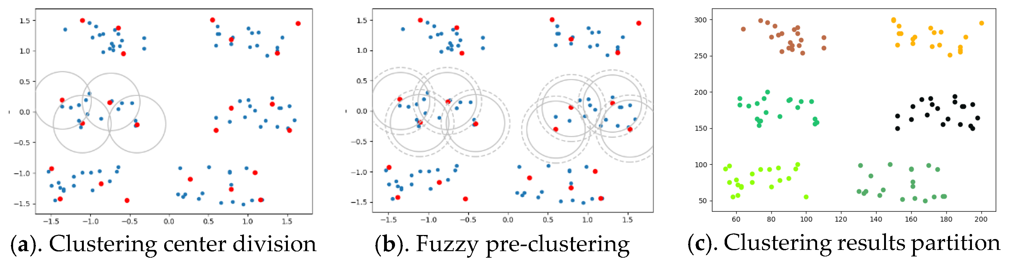
In the behavior of population reproduction and population fusion in nature, it is assumed that there are initially n non-adjacent population origin points. Then new individuals are born near the origin point, and the points close to the origin point are divided into points where races multiply. This cycle continues until all data points have been divided. At this point, the reproduction process ends, and the population fusion process begins. Since data points can belong to multiple populations in the process of dividing, there are common data points between different populations. When the common points between the populations reach a certain number, the populations merge. On the basis of this idea, this section designs and implements an improved hierarchical clustering algorithm with two clustering stages denoted as the PRI-MFC algorithm. The general process of the clustering division of the PRI-MFC is shown in Figure 1.

In the fuzzy pre-clustering stage, based on the neighborhood knowledge of DBSCAN clustering, starting from any point in the overall data, through the neighborhood radius eps, multiple initial cluster center points (Suppose there are k) are divided in turn, and the non-center points are divided into the corresponding cluster centers with eps as the neighborhood radius, as shown in the Figure 1a. The red point in the figure is the cluster center point, and the solid line is the initial clustering. Once again, the non-central data points are divided into k cluster centers according to the neighborhood dispersion radius eps*fog. The same data point can be divided into multiple clusters, and finally, k clusters are formed to complete the fuzzy pre-clustering process. This process is shown in Figure 1b. The radius of the circle drawn by the dotted line in the figure is eps*fog, and the point of the overlapping part between the dotted circles is the common point to be divided. The Euclidean distance is used to determine the similarity of two data points, and the membership grade of a cluster to which the common point belongs is recorded. The Euclidean distance between the common point d_i and the center point c_i divided by eps*fog is the membership grade of ci to which d_i belongs. The neighborhood radius eps is taken from the definition of ε-neighborhood proposed by Stevens. The algorithm parameter fog is the dispersion grade. By setting fog, the overlapping degree of the initial clusters in the algorithm can be adjusted to avoid the misjudgment of outliers. The value range of the parameter fog is [1, 2.5].

In the Jaccard fusion clustering stage, the information of the common points of the clusters is counted and sorted, and the cluster groups to be fused without repeated fusion are found. Then, it sets the parameter jac according to the similarity coefficient of Jaccard to perform the fusion operation on the clusters obtained in the clustering fuzzy pre-clustering stage and obtains several clusters formed by the fusion of m pre-clustering small clusters. The sparse clusters with a data amount of less than three in these clusters are individually marked as outliers to form the final clustering result, as shown in Figure 1c.

The fuzzy pre-clustering of the PRI-MFC algorithm can input data in batches to prevent the situation from running out of memory caused by reading all the data into the memory at one time. The samples in the cluster are divided and stored in the records with unique labels. The pre-clustering process coarsens the original data. In the Jaccard fusion clustering stage, only the number of labels needs to be read to complete the statistics, which reduces the computational complexity of the hierarchical clustering process.

4. Implementation of PRI-MFC Algorithm

This section mainly introduces the steps, flowcharts, and pseudocode of the PRI-MFC algorithm.

4.1. Algorithm Steps and Flow Chart

Combined with optimization strategies [54,55] such as the fuzzy cluster membership grade, coarse-grained data, and staged clustering, the PRI-MFC algorithm reduces the computational complexity of the hierarchical clustering process and improves the execution efficiency of the algorithm. The implementation steps are as follows:

Step 1. Assuming that there are n data points in the data set D, it randomly selects one data point x_i, adds it to the cluster center set centroids, and synchronously builds the cluster dictionary clusters corresponding to the data center centroids set.

Step 2. The remaining n − 1 data points are compared with the points in the centroids, the data points whose distance is greater than the neighborhood radius eps are added to the centroids, and the clusters are updated to obtain all the initial cluster center points in a loop.

Step 3. It performs clustering based on centroids and divides the data points x_i in the data set D whose distance from the cluster center point c_i is less than eps*fog to the clusters with c_i as the cluster center. In the process, if x_i belongs to multiple clusters, it marks it as the point to be fused and records its belonging cluster k and membership grade in the fusion information statistical dictionary match_dic.

Step 4. It counts the number of common points between the clusters, merges the clusters to be fused with repeated clusters to be fused, and calculates the Jaccard similarity coefficient between the clusters to be fused.

Step 5. It fuses the clusters whose similarity between clusters is greater than the fusion parameter jac and divides the common points of the clusters whose similarity between clusters is less than the fusion parameter jac into the cluster with the largest membership grade.

Step 6. In the clustering result obtained in step 5, the clusters with less than three data in the cluster are classified as outliers.

Step 7. The clustering is completed, and the clustering result is output.

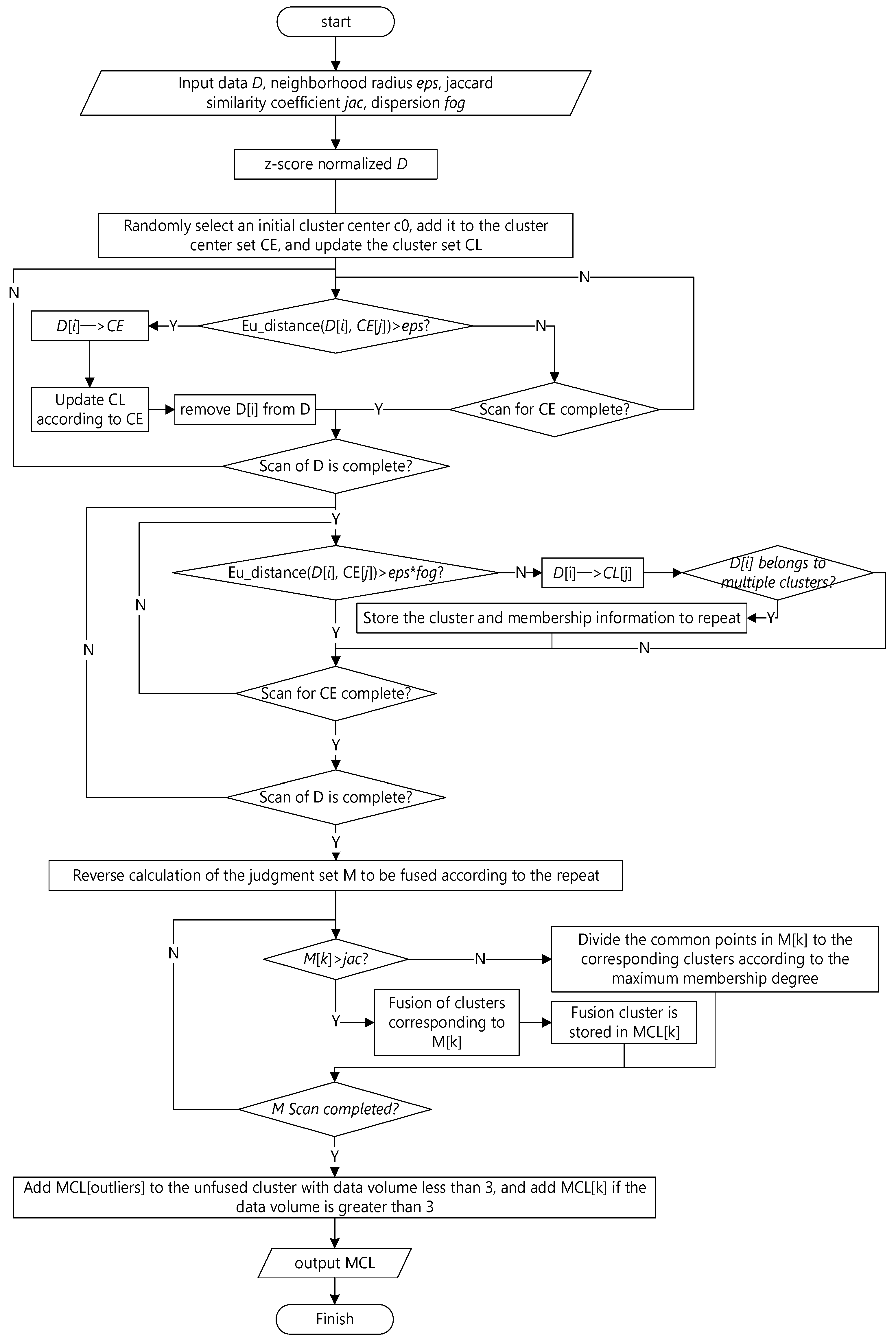
Through the description of the above algorithm steps, the obtained PRI-MFC algorithm flowchart is shown in Figure 2.

4.2. Pseudocode of the Improved Algorithm

The pseudo-code of the PRI-MFC Algorithm 1 is as follows:

Algorithm 1 PRI-MFC
Input: Data D, Neighborhood radius eps, Jaccard similarity coefficient jac, Dispersion fog
Output: Clustering results
1	X = read(D) // read data into X
2	Zscore(X) // data normalization
3	for x0 to xn
4		if x0 then
5			x0 divided into the cluster center set as the first cluster center centers
6			Delete x0 from X and added it into cluster[0]
7		else
8			if Eu_distance(xi, cj) > eps then
9				xi as the j_th clustering center divided into centers
10				Delete xi from X, and added it into cluster
11			end if
12	end for
13	for x0 to xn
14		if Eu_distance(xi, cj) < eps*fog then
15			xi divided into cluster
16			if xi ∈ multi clustering centers then
17				Recode the Membership information of xi to public point collection repeat
18			end if
19		end if
20	end for
21	According to the information in repeat, reversely count the number of common points between each cluster, save to merge
22	for m0 to mk // scan the cluster group to be fused in merge
23		if the public points of group mi > jac then
24			Merge the clusters in group mi, and save it into new clusters
25		else
26			Divide them into corresponding clusters according to the maximum membership grade
27	Mark clusters with less than 3 data within clusters as outliers, save in outliers
28	end for
29	return clusters

5. Experimental Comparative Analysis of PRI-MFC Algorithm

This section introduces the evaluation metrics to measure the quality of the clustering algorithm, designs a variety of experimental methods for different data sets, and illustrates the superiority of the PRI-MFC algorithm by analyzing the experimental results from multiple perspectives.

5.1. Cluster Evaluation Metrics

The experiments in this paper use Accuracy (ACC) [56], Normalized Mutual Information (NMI) [57], and the Adjusted Rand Index (ARI) [58] to evaluate the performance of the clustering algorithm.

The accuracy of the clustering is also often referred to as the clustering purity (purity). The general idea is to divide the number of correctly clustered samples by the total number of samples. However, for the results after clustering, the true category corresponding to each cluster is unknown, so it is necessary to take the maximum value in each case, and the calculation method is shown in Formula (6).

$$\mathrm{ACC}(\mathsf{\Omega },C)=\frac{1}{N}{\displaystyle \sum _k{\max }_j}\left|w_k\cap c_j\right|$$

(6)

Among them, N is the total number of samples, Ω = {w₁, w₂, …, w_k} represents the classification of the samples in the cluster, C = {c₁, c₂, …, c_j} represents the real class of the samples, w_k denotes all samples in the k-th cluster after clustering, and c_j denotes the real samples in the j-th class. The value range of ACC is [0, 1], and the larger the value, the better the clustering result.

Normalized Mutual Information (NMI), that is, the normalization of the mutual information score, can adjust the result between 0 and 1 using the entropy as the denominator. For the true label, A, of the class in the data sets and a certain clustering result, B, the unique value in A is extracted to form a vector, C, and the unique value in B is extracted to form a vector, S. The calculation of NMI is shown in Formula (7).

$${\rm N}{\rm M}{\rm I}(A,B)=\frac{I(C,S)}{\sqrt{H(C)\times H(S)}}$$

(7)

Among them, I(C, S) is the mutual information of the two vectors, C and S, and H(C) is the information entropy of the C vector. The calculation formulas are shown in Formulas (8) and (9). NMI is often used in clustering to measure the similarity of two clustering results. The closer the value is to 1, the better the clustering results.

$$I(C,S)={\displaystyle \sum _{y\in S}{\displaystyle \sum _{x\in C}\log }}\left(\frac{p(c,s)}{p(c)p(s)}\right)$$

(8)

$$H(C)=-{\displaystyle \sum _1^{n}p}\left({\mathrm{c}}_i\right){\log }_{2}p\left(c_i\right)$$

(9)

Adjusted Rand Index (ARI) assumes that the super-distribution of the model is a random model, that is, the division of X and Y is random, and the number of data points for each category and each cluster is fixed. To calculate this value, first calculate the contingency table, as shown in

Table 1. Contingency table.

	X1	X2	…	Xs	Sum
Y1	n11	n12	…	n1s	a1
Y2	n21	n22	…	n2s	a2
…	…	…	…	…	…
Yr	nr1	nr2	…	nrs	ar
sum	b1	b2	…	bs

.

The rows in the table represent the actual divided categories, the columns of the table represent the cluster labels of the clustering division, and each value n_ij represents the number of files in both class(Y) and class(X) at the same time. Calculate the value of ARI through this table. The calculation formula of ARI is shown in Formula (10).

$$\mathrm{ARI}(X,Y)=\frac{{\displaystyle \sum _{ij}\left(\begin{array}{c}{n}_{ij}\\ 2\end{array}\right)}-\left[{\displaystyle \sum _i\left(\begin{array}{c}{a}_i\\ 2\end{array}\right)}{\displaystyle \sum _j\left(\begin{array}{c}{b}_j\\ 2\end{array}\right)}\right]/\left(\begin{array}{c}{n}_2\end{array}\right)}{\frac{1}{2}\left[{\displaystyle \sum _i\left(\begin{array}{c}{a}_i\\ 2\end{array}\right)}+{\displaystyle \sum _j\left(\begin{array}{c}{b}_j\\ 2\end{array}\right)}\right]-\left[{\displaystyle \sum _i\left(\begin{array}{c}{a}_i\\ 2\end{array}\right)}{\displaystyle \sum _j\left(\begin{array}{c}{b}_j\\ 2\end{array}\right)}\right]/\left(\begin{array}{c}n\\ 2\end{array}\right)}$$

(10)

The value range of ARI is [−1, 1], and the larger the value, the more consistent the clustering results are with the real situation.

5.2. Experimental Data

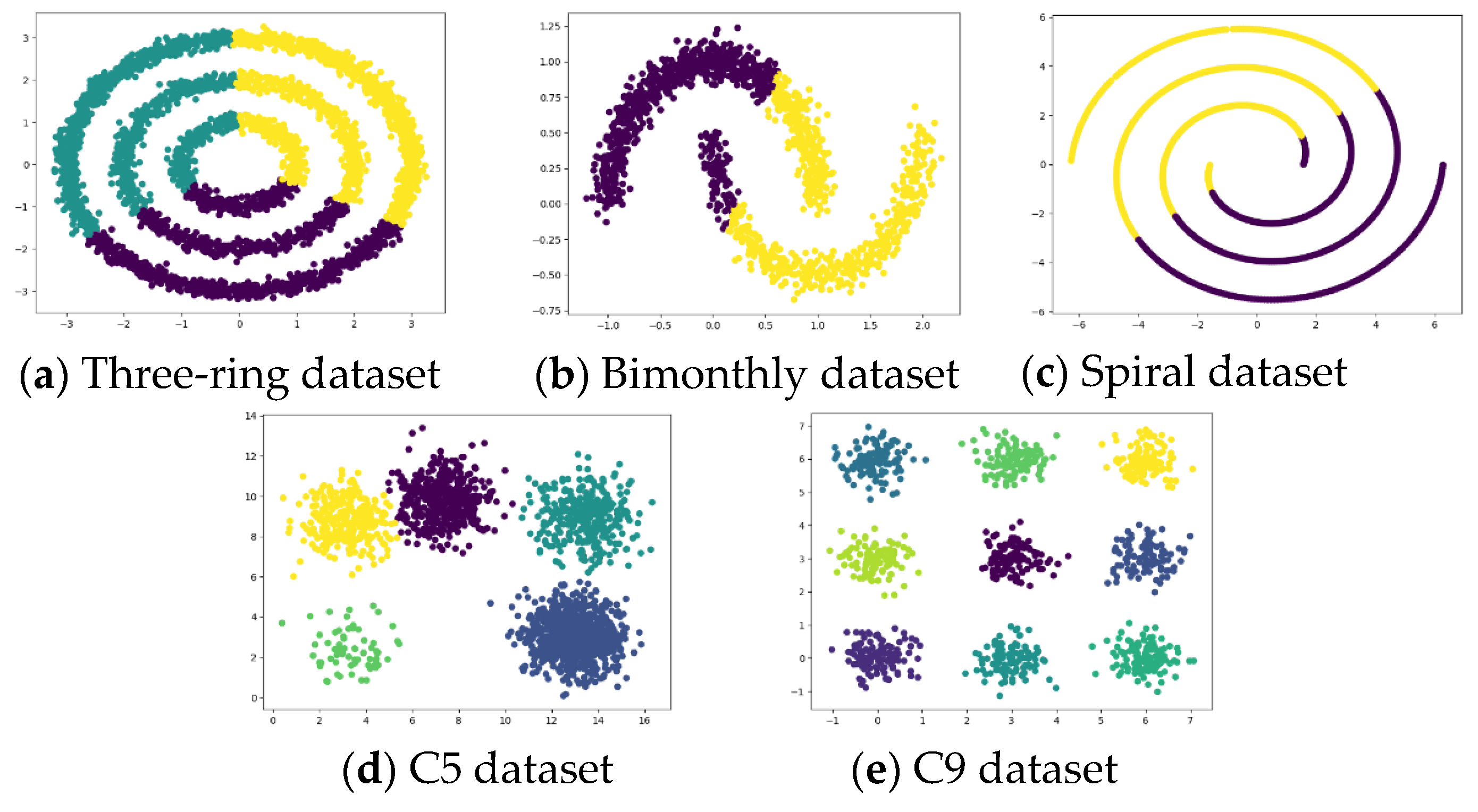
For algorithm performance testing, the experiments use five simulated datasets, as shown in

Table 2. Artificial datasets.

Serial Number	Datasets	Sample	Feature	Number of Clusters
D1	Three-ring	3600	2	3
D2	Bimonthly	1500	2	2
D3	Spiral	941	2	2
D4	C5	2000	2	5
D5	C9	1009	2	9

. The tricyclic datasets, bimonthly datasets, and spiral datasets are used to test the clustering effect of the algorithm on irregular clusters, and the C5 datasets and C9 datasets are used to test the clustering effect of the algorithm on common clusters.

In addition, the algorithm performance comparison experiment also uses six UCI real datasets, including Seeds datasets. The details of the data are shown in

Table 3. UCI datasets.

Serial Number	Datasets	Sample	Feature	Number of Clusters
D1	Seeds	210	7	3
D2	Iris	150	4	3
D3	Breast	699	10	2
D4	Glass	214	9	6
D5	Ecoli	336	7	7
D6	Pima	768	9	2

.

5.3. Analysis of Experimental Results

This section contains experiments on the PRI-MFC algorithm on artificial datasets, various UCI datasets, and the China Financial Household Survey datasets.

5.3.1. Experiments on Artificial Datasets

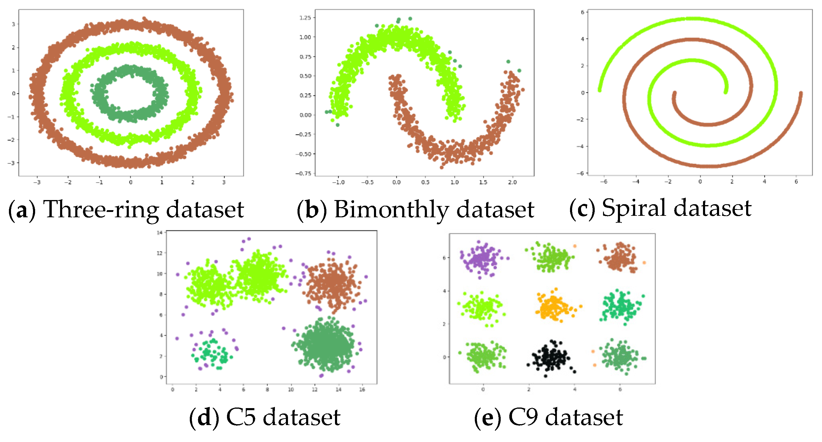
The K-means algorithm [53] and the PRI-MFC algorithm are used for experiments on datasets shown in Table 1, and the experimental clustering results are visualized as shown in Figure 3 and Figure 4, respectively.

It can be seen from the figure that the clustering effect of K-means on the tricyclic datasets, bimonthly datasets, and spiral datasets with uniform density distribution is not ideal. However, K-means has a good clustering effect on both C5 datasets and C9 datasets with uneven density distribution. The PRI-MFC algorithm has a good clustering effect on the three-ring datasets, bimonthly datasets, spiral datasets, and C9 datasets. While accurately clustering the data, it more accurately marks the outliers in the data. However, it fails to distinguish adjacent clusters on the C5 datasets, and the clustering effect is poor for clusters with insignificant clusters in the data.

Comparing the clustering results of the two algorithms, it can be seen that the clustering effect of the PRI-MFC algorithm is better than that of the K-means algorithm on most of the experimental datasets. The PRI-MFC algorithm is not only effective on datasets with uniform density distributions but also has better clustering effects on datasets with large differences in density distributions.

5.3.2. Experiments on UCI Datasets

In this section, experiments on PRI-MFC, K-means [1], ISODATA [59], DBSCAN, and KMM [1] are carried out on various UCI datasets to verify the superiority of the PRI-MFC from the perspective of clustering quality, time, and algorithm parameter influence.

Clustering Quality Perspective

On the UCI data set, PRI-MFC is compared with K-means, ISODATA, DBSCAN, and KMM, and the evaluation index values of the clustering results on various UCI data sets are obtained, which are the accuracy rate (ACC), the standardized mutual information (NMI), and the adjusted Rand coefficient (ARI). The specific experimental results are shown in

Table 4. Clustering evaluation index values of five algorithms on the UCI datasets(%).

Datasets	Evaluation Metrics	K-Means	DBSCAN	ISODATA	KMM	PRI-MFC
Seeds	ACC	90.95	59.04	35.71	62.86	66.66
	NMI	70.88	52	76.81	58.16	64.68
	ARI	75.05	39.49	73.98	49.69	51.44
Iris	ACC	30.67	33.33	56.81	36.67	66.66
	NMI	0.8	0.33	73.37	0.44	73.36
	ARI	0.42	0.64	56.81	0.33	76.81
Breast	ACC	96.05	64.57	41.29	1.17	95.16
	NMI	74.68	10.54	2.22	79.21	76.64
	ARI	84.65	9.60	−2.74	87.98	85.43
Glass	ACC	51.87	42.52	50	32.71	34.11
	NMI	42.37	36.07	66.17	28.55	42.19
	ARI	27.66	22.26	48.76	14.10	27.52
Ecoli	ACC	56.55	42.56	73.51	0.89	57.35
	NMI	58.38	11.31	73.63	44.17	61.97
	ARI	46.50	3.80	78.45	36.99	75.34
Pima	ACC	67.19	63.80	32.94	34.51	35.28
	NMI	6.07	0.0	0.31	0.25	6.03
	ARI	11.07	0.13	−0.54	0.43	9.08

.

In order to better observe the clustering quality, the evaluation index data in Table 4 are assigned weight values 5, 4, 3, 2, and 1 in descending order. The ACC index values of the five algorithms on the UCI datasets are shown in

Table 5. ACC index values of five algorithms on the UCI datasets (%).

Datasets	K-Means	DBSCAN	ISODATA	KMM	PRI-MFC
Seeds	90.95	59.04	35.71	63.31	74.28
Iris	30.67	34.62	56.81	37.33	69.74
Breast	96.05	64.57	41.29	56.95	95.16
Glass	51.87	42.52	50	35.04	34.11
Ecoli	56.55	42.56	73.51	47.32	57.35
Pima	67.19	63.8	32.94	60.15	35.28

, and the weight values assigned to the ACC index values are shown in

Table 6. The weight values of the ACC of five algorithms on the UCI datasets.

Datasets	K-Means	DBSCAN	ISODATA	KMM	PRI-MFC
Seeds	5	2	1	3	4
Iris	1	2	4	3	5
Breast	5	3	1	2	4
Glass	5	3	4	2	1
Ecoli	3	1	5	2	4
Pima	5	4	1	3	2

. Taking the ACC of K-means as an example, the weighted average of the ACC of K-means is (90.95 × 5 + 30.67 × 1 + 96.05 × 5 + 51.87 × 5 + 56.55 × 3 + 67.19 × 5)/24 = 72.11. Calculated in this way, the weighted average of each algorithm evaluation index is obtained as shown in

Table 7. The weighted averages of the evaluation index of five algorithms (%).

Evaluation Metrics	K-Means	DBSCAN	ISODATA	KMM	PRI-MFC
ACC	72.11	53.76	56.55	50.73	68.03
NMI	40.22	19.61	60.54	45.05	54.21
ARI	42.52	9.93	57.8	44.93	56.54

.

From Table 7, the weighted average of ACC of K-means is 0.7211 and the weighted average of ACC of PRI-MFC is 0.6803. From the perspective of ACC, the K-means algorithm is the best, and the PRI-MFC algorithm is better. The weighted average of NMI of ISODATA is 0.6054, and the weighted average of NMI of the PRI-MFC algorithm is 0.5424. From the perspective of NMI, the PRI-MFC algorithm is better. Similarly, it can also be seen that the PRI-MFC algorithm has a better effect from the perspective of ARI.

In order to comprehensively consider the quality of the five clustering algorithms, weights 5, 4, 3, 2, and 1 are assigned to each evaluation index data in Table 7 in descending order, and the result is shown in

Table 8. The weight values of the weighted averages of the evaluation index of five algorithms.

Evaluation Metrics	K-Means	DBSCAN	ISODATA	KMM	PRI-MFC
ACC	5	2	3	1	4
NMI	2	1	5	3	4
ARI	2	1	5	3	4

.

The weighted average of the comprehensive evaluation index of each algorithm is calculated according to the above method, and the result is shown as

Table 9. The weighted averages of comprehensive evaluation index of five algorithms (%).

Evaluation Metrics	K-Means	DBSCAN	ISODATA	KMM	PRI-MFC
comprehensive evaluation index	56.91	34.27	58.57	44.93	58.76

. It can be seen that the PRI-MFC algorithm proposed in this paper is the best in terms of clustering quality.

Time Perspective

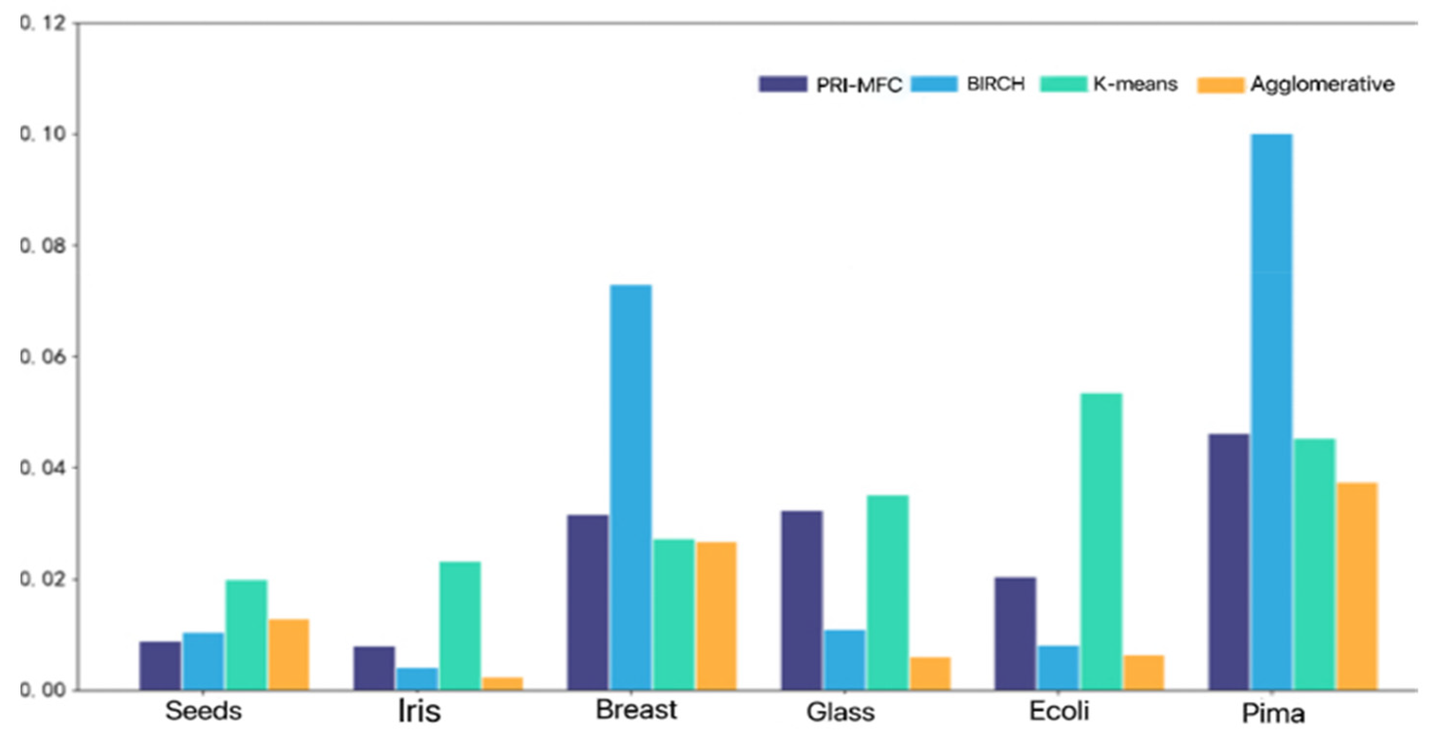
In order to illustrate the superiority of the algorithm proposed in this paper, the PRI-MFC algorithm, the classical partition-based clustering algorithm, K-means, the commonly used hierarchical clustering algorithm, BIRCH, and Agglomerative are tested on six real data sets, respectively, as shown in Figure 5.

The BIRCH algorithm takes the longest time, with an average time of 34.5 ms. The K-means algorithm takes second place, with an average time of 34.07 ms. The PRI-MFC algorithm takes a shorter time, with an average time of 24.59 ms, and Agglomerative is the shortest, with an average time-consuming of 15.35 ms. The PRI-MFC clustering algorithm wastes time in fuzzy clustering processing so it takes a little longer than Agglomerative. However, the PRI-MFC algorithm only needs to read the number of labels in the Jaccard fusion clustering stage to complete the statistics which saves time. The overall time consumption is shorter than the other algorithms.

Algorithm Parameter Influence Angle

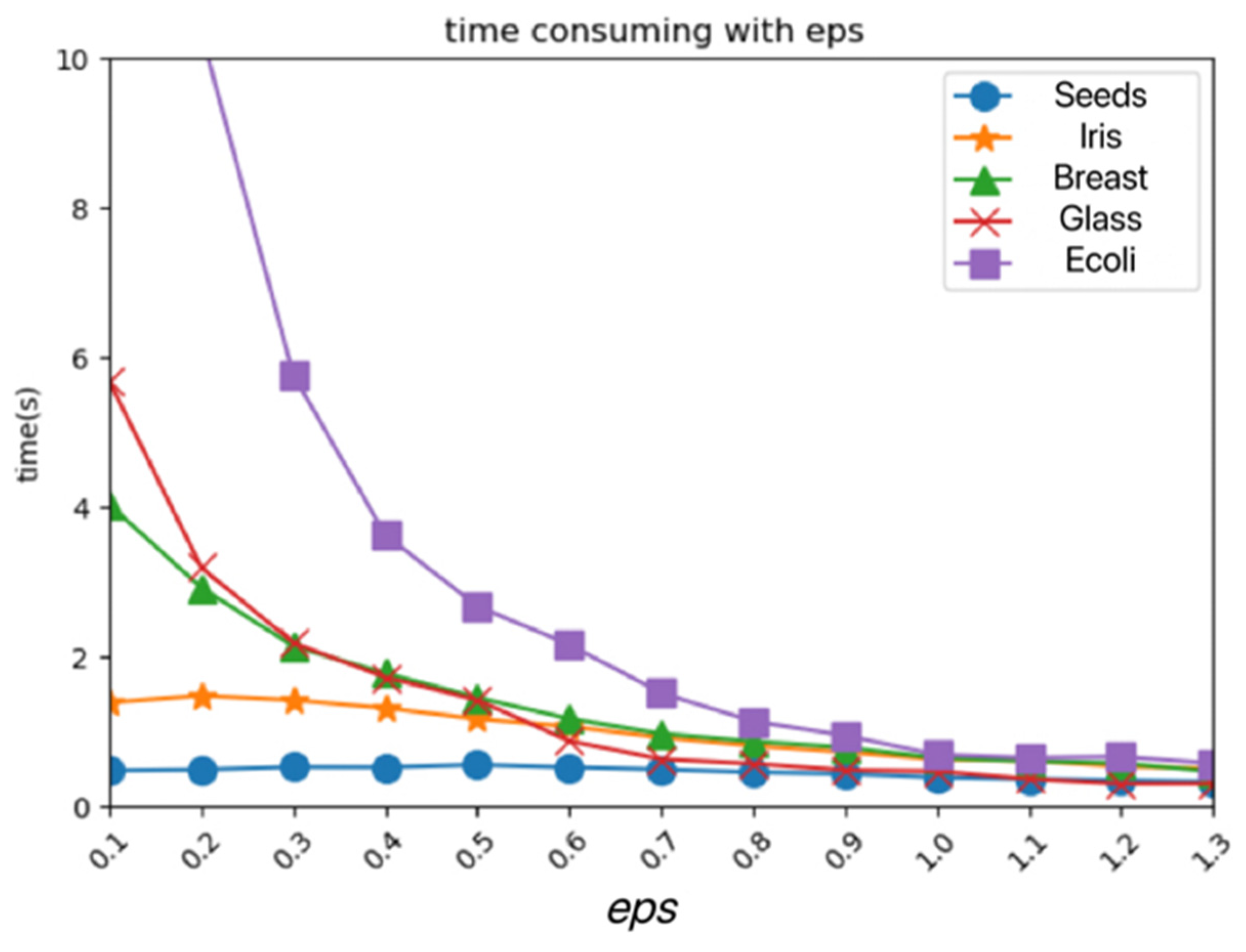
In this section, the PRI-MFC algorithm is tested on UCI, and the eps parameter value is modified. The time consumption of the PRI-MFC is shown in Figure 6. It can be seen that with an increase in the eps parameter value, the time consumption of the algorithm decreases again. It can be seen that the time of the algorithm is negatively correlated with the eps parameter. In the fuzzy pre-clustering stage of the PRI-MFC algorithm, the influence of the eps parameter on the time consumption of the algorithm is more obvious.

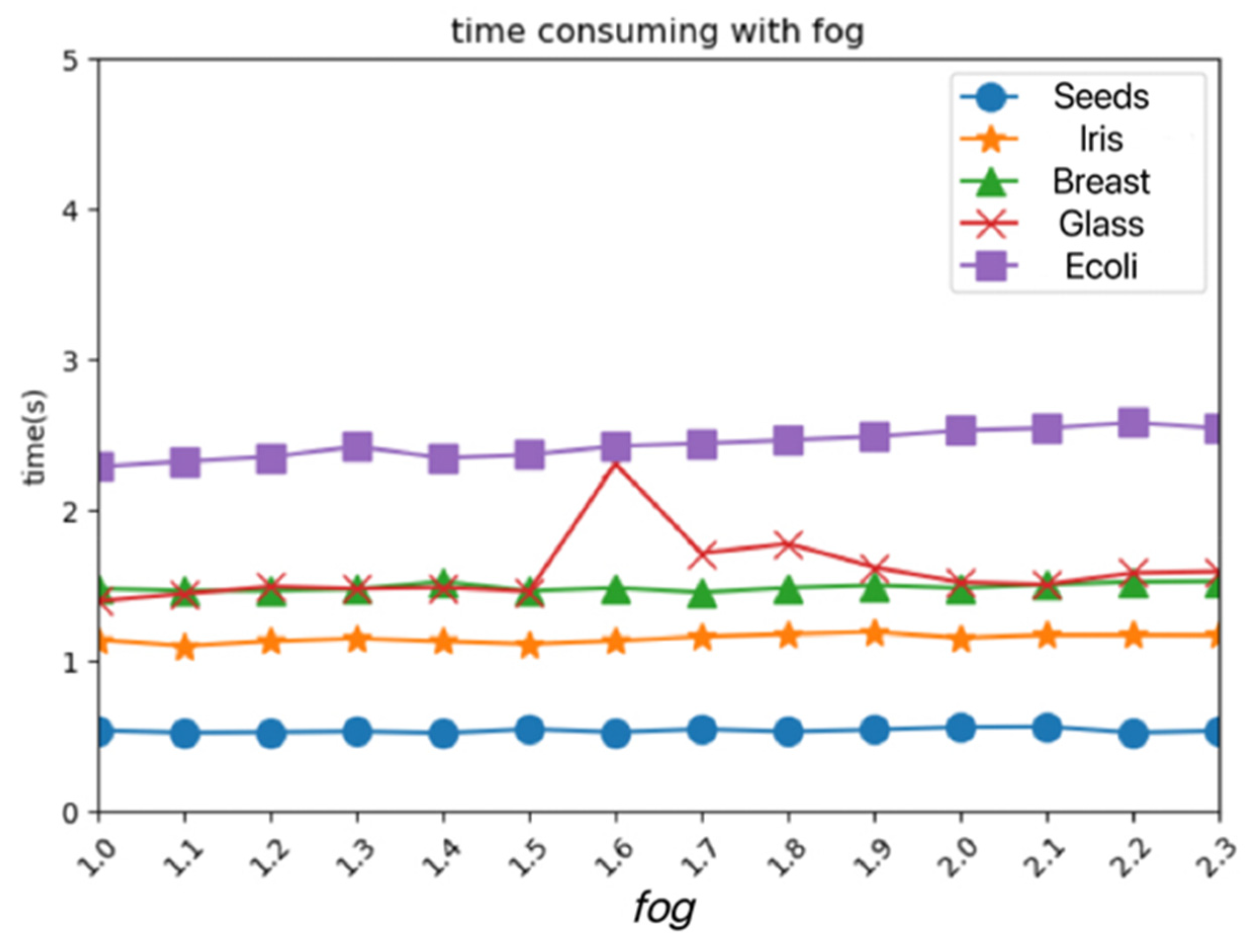
After modifying the fog parameter value, the time consumption of the PRI-MFC algorithm is shown in Figure 7. It can be seen that, with the increase of the fog parameter value, the time consumption of the algorithm increases again. It can be seen that the time of the algorithm is positively correlated with the fog parameter.

5.3.3. Experiments on China’s Financial Household Survey Data

The similarity of the hierarchical clustering algorithm is easy to define. It does not need to pre-determine the number of clusters. It can discover the hierarchical relationship of the classes and cluster them into various shapes, which is suitable for community analysis and market analysis [60]. In this section, the PRI-MFC algorithm conducts experiments on real Chinese financial household survey data, displays the clustering results, and then analyzes the household financial community to demonstrate the practicability of this algorithm.

Datasets

This section uses the 2019 China Household Finance Survey data, which covers 29 provinces (autonomous regions and municipalities), 343 districts and counties, and 1360 village (neighborhood) committees. Finally, the information of 34,643 households and 107,008 family members is collected. The data are nationally and provincially representative, including three datasets: family datasets, personal datasets, and master datasets. The data details are shown in

Table 10. China household finance survey data details from 2019.

Data Name	The Amount of Data	Attributes
family data	34,643	2656
Personal data	107,008	423
master data	107,008	54

.

The attributes that have high values for the family financial group clustering experiment in the three data sets are selected, redundant irrelevant attributes are deleted, and then duplicate data are removed, and the family data set and master data set are combined into a family data set. The preprocessed data are shown in

Table 11. Preprocessed China household finance survey data.

Data Name	The Amount of Data	Attributes
Family	34,643	53
Personal	107,008	13

.

Experiment

The experiments of the PRI-MFC algorithm are carried out on the two data sets in Table 11. The family data table has a total of 34,643 pieces of data and 53 features, of which there are 16,477 pieces of household data without debt. First, the household data of debt-free urban residents are selected to conduct the PRI-MFC algorithm experiment. The data features are selected as total assets, total household consumption, and total household income. Since there are 28 missing values in each feature of the data, there are 9373 actual experimental data. Secondly, the household data of non-debt rural residents are selected. The selected data features are the same as above. There are 10 missing values for each feature of these data, and the actual experimental data have a total of 7066 items. The clustering results obtained from the two experiments are shown in

Table 12. Financial micro-data clustering of Chinese debt-free households.

Area	Cluster	Sample	Proportion (%)	Mean 1	Mean 2	Mean 3	Tag
Town	1	8179	87.26	672,405.82	67,649.73	73,863.01	Well-off
	2	1047	11.17	4,454,086.8	130,084.35	185,686.23	Middle
	3	144	1.53	10,647,847.47	239,064.97	390,016.64	Rich
Rural	1	6956	98.44	307,014.13	52,879.74	41,349.55	Well-off
	2	105	1.48	4,647,506.43	113,648.82	228,253.08	Middle
	3	5	0.07	20,590,783.60	66,631.20	69,243.30	Rich

.

It can be seen from Table 12 that regardless of urban or rural areas, the population in my country can be roughly divided into three categories: well-off, middle-class, and affluent. The clustering results are basically consistent with the distribution of population income in my country. The total income of middle-class households in urban areas is lower than that of middle-class households in rural areas, but their expenditures are lower and their total assets are higher. It can be seen that the fixed asset value of the urban population is higher, the fixed asset value of the rural population is lower, and the well-off households account for the highest proportion of the total rural households, accounting for 98.44%. Obviously, urban people and a small number of rural people have investment needs, but only a few wealthy families can have professional financial advisors. Most families have minimal financial knowledge and do not know much about asset appreciation and maintaining capital value stability. This clustering result is beneficial for financial managers to make decisions and bring them more benefits.

5.4. Discussion

The experiment on artificial datasets shows that the clustering effect of the PRI-MFC algorithm is better than that of the classical partitioned K-means algorithm regardless of whether the data density is uniform or not. Because the first stage of PRI-MFC algorithm clustering relies on the idea of density clustering, it can cluster uneven density data. Experiments were carried out on the real data set from three aspects: clustering quality, time consumption, and parameter influence. The evaluation metrics of ACC, NMI, and ARI of the five algorithms obtained in the experiment were further analyzed. Calculating the weighted average of each evaluation index of each algorithm, the experiment concludes that the clustering quality of the PRI-MFC algorithm is better. The weighted average of the comprehensive evaluation index of each algorithm was further calculated, and it was concluded that the PRI-MFC algorithm is optimal in terms of clustering quality. The time consumption of each algorithm is displayed through the histogram. The PRI-MFC clustering algorithm wastes time in fuzzy clustering processing, and its time consumption is slightly longer than that of Agglomerative. However, in the Jaccard fusion clustering stage, the PRI-MFC algorithm only needs to read the number of labels to complete the statistics, which saves time, and the overall time consumption is less than other algorithms. Experiments from the perspective of parameters show that the time of this algorithm has a negative correlation with the parameter eps and a positive correlation with the parameter fog. When the parameter eps changes from large to small in the interval [0, 0.4], the time consumption of the algorithm increases rapidly. When the eps parameter changes from large to small in the interval [0.4, 0.8], the time consumption of the algorithm increases slowly. When the eps parameter in the interval between [0.8, 1.3] changes from large to small, the time consumption of the algorithm tends to be stable. In conclusion, from the perspective of the clustering effect and time consumption, the algorithm is better when the eps is 0.8. When the fog parameter is set to 1, the time consumption is the lowest, because the neighborhood radius and the dispersion radius are the same at this time. With the increase of the fog value, the time consumption of the algorithm gradually increases. In conclusion, from the perspective of the clustering effect and time consumption, the algorithm is better when fog is set to 1.8. Experiments conducted on Chinese household finance survey data show that the PRI-MFC algorithm is practical and can be applied in market analysis, community analysis, etc.

6. Conclusions

In view of the problems that the traditional hierarchical clustering algorithm cannot find clusters with uneven density, requires a large amount of calculation and has low efficiency, this paper takes advantage of the benefits of the classical hierarchical clustering algorithm and the advantages of the DBSCAN algorithm for clustering data with uneven density. Based on population reproduction and fusion, a new hierarchical clustering algorithm PRI-MFC is proposed. This algorithm can effectively identify clusters of any shape, and preferentially identify cluster-dense centers. It can effectively remove noise in samples and reduce outlier pairs by clustering and re-integrating multiple cluster centers. By setting different parameters for eps and fog, the granularity of clustering can be adjusted. Secondly, various experiments are designed on artificial datasets and real datasets, and the results show that this algorithm is better in terms of clustering effect, clustering quality, and time consumption. Due to the uncertainty of objective world data, the next step is to study the fuzzy hierarchical clustering algorithm further. With the advent of the era of big data, running the algorithm on a single computer is prone to bottleneck problems. The next step is to study the improvement of clustering algorithms under the big data platform.