
Low-Complexity Acoustic Scene Classification Using Time Frequency Separable Convolution

Abstract
:1. Introduction
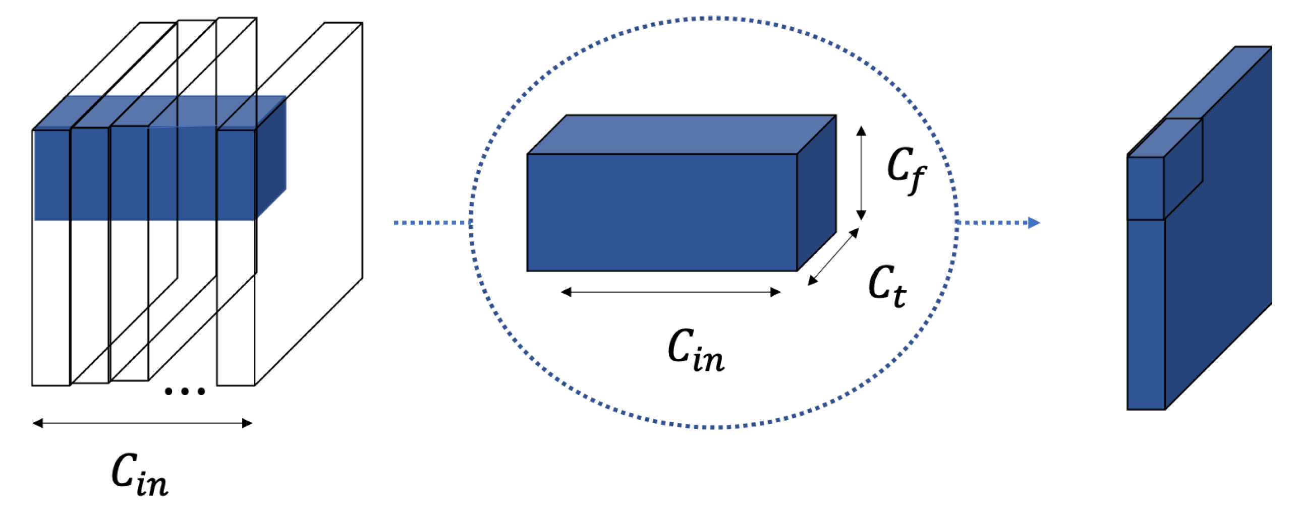
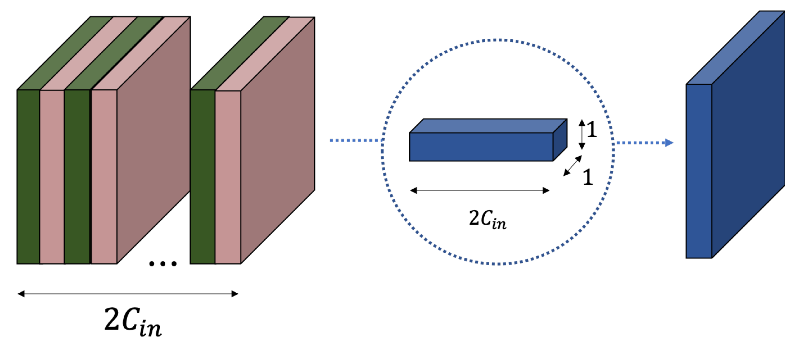
2. Time-Frequency Separable Convolution
3. Experiment with CNN-Based Network
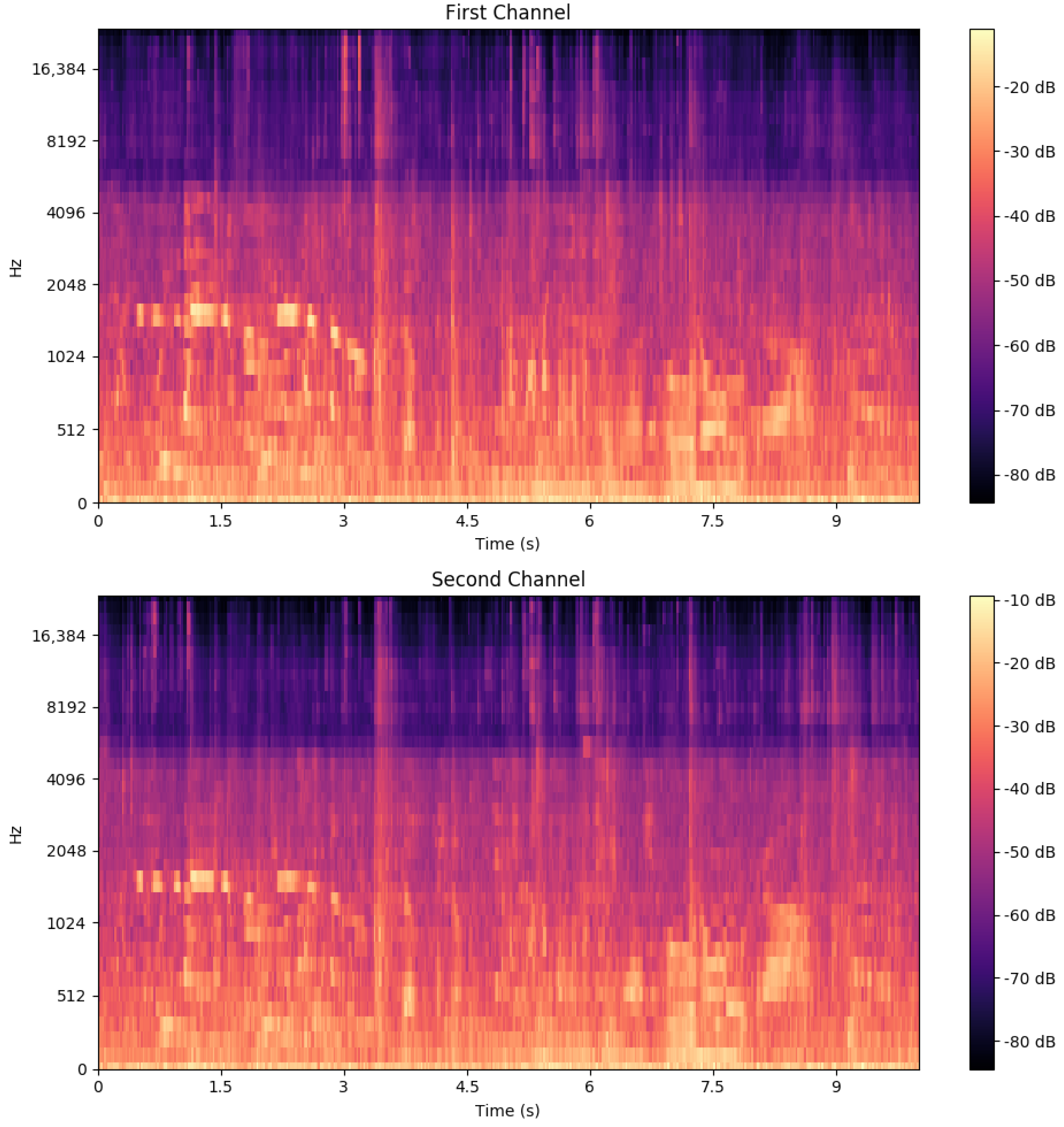
3.1. Dataset
3.2. CNN Baseline Architecture
3.3. Proposed Architecture
3.4. Experiment Setup
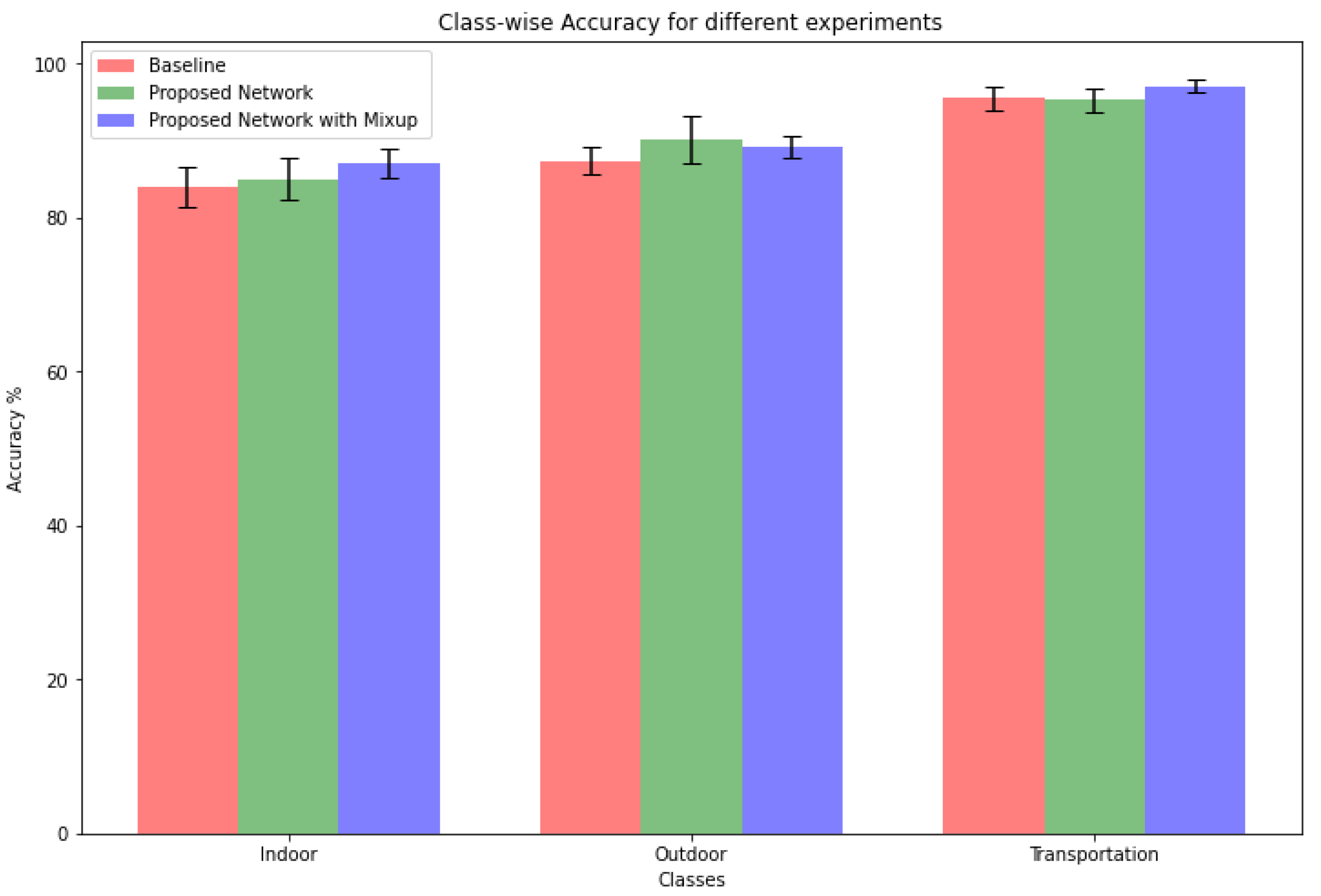
3.5. Performance
4. Experiment with Resnet Based Network
4.1. Dataset
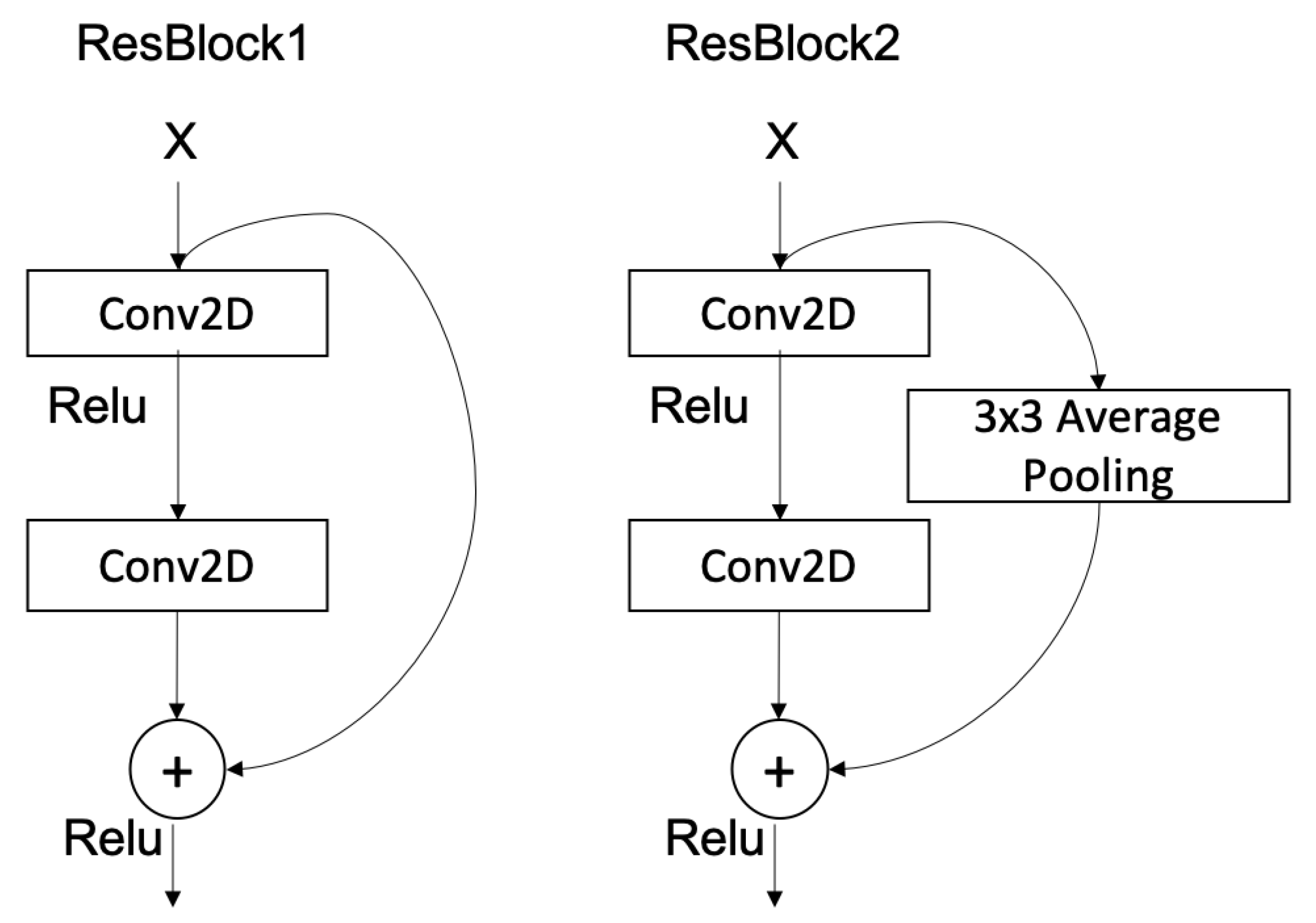
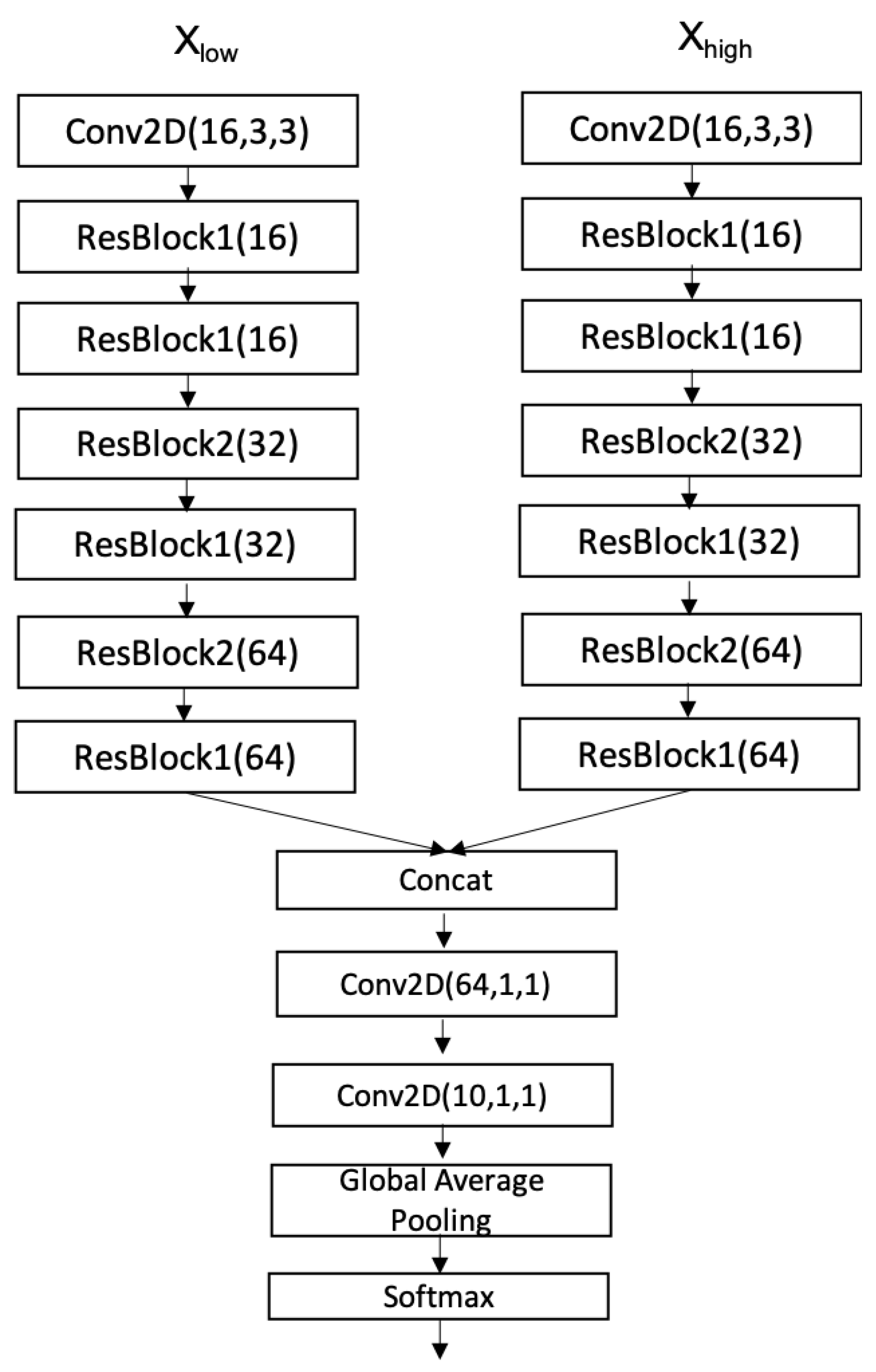
4.2. ResNet Baseline Model
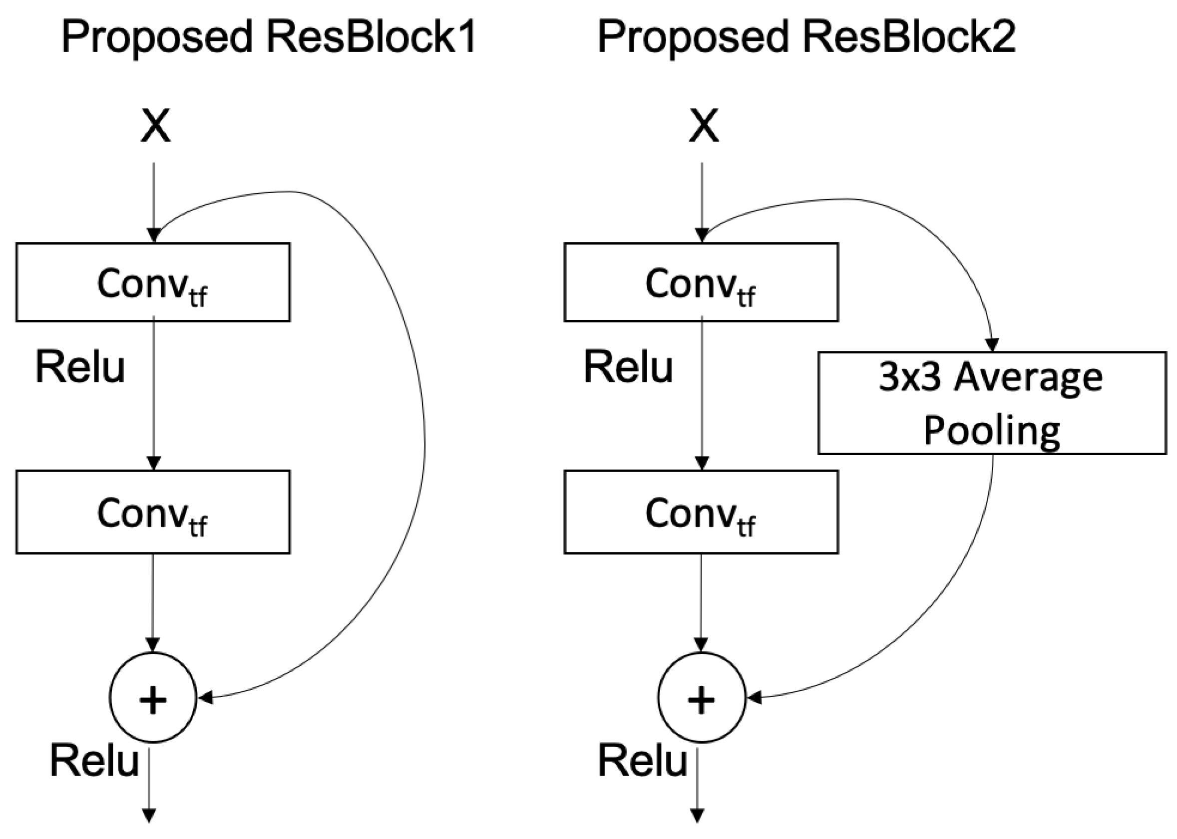
4.3. Compressed-ResNet Model
4.4. Experiment
4.5. Performance
5. Discussions and Conclusions
Author Contributions
Funding
Institutional Review Board Statement
Informed Consent Statement
Data Availability Statement
Acknowledgments
Conflicts of Interest
References
- Abeßer, J. A review of deep learning based methods for acoustic scene classification. Appl. Sci. 2020, 10, 2020. [Google Scholar] [CrossRef] [Green Version]
- Jung, J.W.; Heo, H.S.; Shim, H.J.; Yu, H.J. Knowledge Distillation in Acoustic Scene Classification. IEEE Access 2020, 8, 166870–166879. [Google Scholar]
- Basbug, A.M.; Sert, M. Acoustic scene classification using spatial pyramid pooling with convolutional neural networks. In Proceedings of the 2019 IEEE 13th International Conference on Semantic Computing (ICSC), Newport Beach, CA, USA, 30 January–1 February 2019; pp. 128–131. [Google Scholar]
- Khamparia, A.; Singh, K.M. A systematic review on deep learning architectures and applications. Expert Syst. 2019, 36, e12400. [Google Scholar]
- Zeinali, H.; Burget, L.; Cernocky, J. Convolutional neural networks and x-vector embedding for DCASE2018 acoustic scene classification challenge. arXiv 2018, arXiv:1810.04273. [Google Scholar]
- Koutini, K.; Eghbal-zadeh, H.; Widmer, G. Receptive-Field-Regularized CNN Variants For Acoustic Scence classification. In Proceedings of the Acoustic Scenes and Events 2019 Workshop (DCASE2019), New York, NY, USA, 25–26 October 2019; p. 124. [Google Scholar]
- Mesaros, A.; Heittola, T.; Virtanen, T. Acoustic scene classification in DCASE 2019 Challenge: Closed and open set classification and data mismatch setups. In Proceedings of the Workshop on Detection and Classification of Acoustic Scenes and Events, New York, NY, USA, 25–26 October 2019. [Google Scholar]
- Heittola, T.; Mesaros, A.; Virtanen, T. Acoustic scene classification in DCASE 2020 Challenge: Generalization across devices and low complexity solutions. In Proceedings of the Workshop on Detection and Classification of Acoustic Scenes and Events, Virtual, 2–4 November 2020; pp. 56–60. [Google Scholar]
- Simonyan, K.; Zisserman, A. Very deep convolutional networks for large-scale image recognition. arXiv 2014, arXiv:1409.1556. [Google Scholar]
- He, K.; Zhang, X.; Ren, S.; Sun, J. Deep residual learning for image recognition. In Proceedings of the IEEE Conference on Computer Vision and Pattern Recognition, Las Vegas, NV, USA, 27–30 June 2016; pp. 770–778. [Google Scholar]
- Huang, G.; Liu, Z.; Van Der Maaten, L.; Weinberger, K.Q. Densely connected convolutional networks. In Proceedings of the IEEE Conference on Computer Vision and Pattern Recognition, Honolulu, HI, USA, 21–26 July 2017; pp. 4700–4708. [Google Scholar]
- Suh, S.; Park, S.; Jeong, Y.; Lee, T. Designing acoustic scene classification models with CNN variants. In DCASE2020 Challenge; Technical Report; 2020; Available online: https://dcase.community/documents/challenge2020/technical_reports/DCASE2020_Suh_101.pdf (accessed on 23 August 2022).
- Howard, A.G.; Zhu, M.; Chen, B.; Kalenichenko, D.; Wang, W.; Weyand, T.; Andreetto, M.; Adam, H. Mobilenets: Efficient convolutional neural networks for mobile vision applications. arXiv 2017, arXiv:1704.04861. [Google Scholar]
- Albawi, S.; Mohammed, T.A.; Al-Zawi, S. Understanding of a convolutional neural network. In Proceedings of the 2017 International Conference on Engineering and Technology (ICET), Antalya, Turkey, 21–23 August 2017; pp. 1–6. [Google Scholar]
- Hinton, G.; Vinyals, O.; Dean, J. Distilling the Knowledge in a Neural Network. Statistics 2015, 1050, 9. [Google Scholar]
- Han, S.; Pool, J.; Tran, J.; Dally, W.J. Learning both weights and connections for efficient neural networks. In Proceedings of the 28th International Conference on Neural Information Processing Systems, Montreal, QC, Canada, 7–12 December 2015; Volume 1, pp. 1135–1143. [Google Scholar]
- Frankle, J.; Carbin, M. The Lottery Ticket Hypothesis: Finding Sparse, Trainable Neural Networks. In Proceedings of the International Conference on Learning Representations, Vancouver, BC, Canada, 30 April–3 May 2018. [Google Scholar]
- Zhu, M.H.; Gupta, S. To prune, or not to prune: Exploring the efficacy of pruning for model compression. Statistics 2017, 1050, 13. [Google Scholar]
- Sandler, M.; Howard, A.; Zhu, M.; Zhmoginov, A.; Chen, L.C. Mobilenetv2: Inverted residuals and linear bottlenecks. In Proceedings of the IEEE Conference on Computer Vision and Pattern Recognition, Salt Lake City, UT, USA, 18–22 June 2018; pp. 4510–4520. [Google Scholar]
- Chollet, F. Xception: Deep learning with depthwise separable convolutions. In Proceedings of the IEEE Conference on Computer Vision and Pattern Recognition (CVPR), Honolulu, HI, USA, 21–26 July 2017; pp. 1251–1258. [Google Scholar]
- Wang, X.; Hersche, M.; Tömekce, B.; Kaya, B.; Magno, M.; Benini, L. An accurate eegnet-based motor-imagery brain–computer interface for low-power edge computing. In Proceedings of the 2020 IEEE International Symposium on Medical Measurements and Applications (MeMeA), Bari, Italy, 1 June–1 July 2020; pp. 1–6. [Google Scholar]
- Schneider, T.; Wang, X.; Hersche, M.; Cavigelli, L.; Benini, L. Q-EEGNet: An energy-efficient 8-bit quantized parallel EEGNet implementation for edge motor-imagery brain-machine interfaces. In Proceedings of the 2020 IEEE International Conference on Smart Computing (SMARTCOMP), Bologna, Italy, 14–17 September 2020; pp. 284–289. [Google Scholar]
- Morato, I.M.; Heittola, T.; Mesaros, A.; Virtanen, T. Low-complexity acoustic scene classification for multi-device audio: Analysis of DCASE 2021 Challenge systems. In Proceedings of the Detection and Classication of Acoustic Scenes and Events, Online, 15 November 2021; pp. 85–89. [Google Scholar]
- Hu, H.; Yang, C.H.H.; Xia, X.; Bai, X.; Tang, X.; Wang, Y.; Niu, S.; Chai, L.; Li, J.; Zhu, H.; et al. A two-stage approach to device-robust acoustic scene classification. In Proceedings of the ICASSP 2021–2021 IEEE International Conference on Acoustics, Speech and Signal Processing (ICASSP), Toronto, ON, Canada, 6–11 June 2021; pp. 845–849. [Google Scholar]
- Goodfellow, I.; Bengio, Y.; Courville, A. Deep Learning; MIT Press: Cambridge, MA, USA, 2016; Available online: http://www.deeplearningbook.org (accessed on 23 August 2022).
- Kingma, D.P.; Ba, J. Adam: A Method for Stochastic Optimization. arXiv 2015, arXiv:1412.6980. [Google Scholar]
- Inoue, H. Data augmentation by pairing samples for images classification. arXiv 2018, arXiv:1801.02929. [Google Scholar]
- Hajek, B. Random Processes for Engineers; Cambridge University Press: Cambridge, UK, 2015. [Google Scholar]


| Layer | Number of Parameters |
|---|---|
| Input | 0 |
| Conv2D(32,7,7) | 3136 |
| Batchnorm | 128 |
| Relu | 0 |
| MaxP(5,5) | 0 |
| Dropout(0.3) | 0 |
| Conv2D(64,7,7) | 100,352 |
| Batchnorm | 256 |
| Relu | 0 |
| MaxP(4,100) | 0 |
| Dropout(0.3) | 0 |
| FC(100) | 12,900 |
| Batchnorm | 400 |
| Relu | 0 |
| Dropout(0.3) | 0 |
| FC(3) | 303 |
| Softmax | 0 |
| Output | 0 |
| Total parameters | 117,475 |
| Layer | Number of Parameters |
|---|---|
| Input | 0 |
| AverageP(1,5) | 0 |
| Conv(32,4,5) | 2980 |
| Batchnorm | 128 |
| Relu | 0 |
| AverageP(2,3) | 0 |
| Conv(64,5,5) | 4672 |
| Batchnorm | 256 |
| Relu | 0 |
| GlobalMaxPooling | 0 |
| FC(3) | 195 |
| Softmax | 0 |
| Output | 0 |
| Total parameters | 8003 |
| System | Number of Parameters | Total Size |
|---|---|---|
| Baseline | 117,475 | 469.9 KB |
| Proposed Structure | 8003 | 32 KB |
| System | Accuracy (%) | Log Loss |
|---|---|---|
| Baseline model | 88.96 ± 0.56 | 0.352 ± 0.064 |
| Proposed model | 90.15 ± 0.77 | 0.293 ± 0.024 |
| Proposed model with mixup | 91.14 ± 0.40 | 0.287 ± 0.006 |
| Model | Total Number of Parameters |
|---|---|
| Baseline ResNet | 363,084 |
| Compressed ResNet | 57,484 |
| System | Accuracy (%) | Log Loss |
|---|---|---|
| DCASE2021 Task 1A Baseline | 47.7 ± 0.9 | 1.473 ± 0.05 |
| Baseline ResNet | 65.99 ± 0.12 | 1.4700 ± 0.0037 |
| Compressed ResNet | 64.65 ± 0.35 | 1.4958 ± 0.0033 |
Publisher’s Note: MDPI stays neutral with regard to jurisdictional claims in published maps and institutional affiliations. |
© 2022 by the authors. Licensee MDPI, Basel, Switzerland. This article is an open access article distributed under the terms and conditions of the Creative Commons Attribution (CC BY) license (https://creativecommons.org/licenses/by/4.0/).
Share and Cite
Phan, D.H.; Jones, D.L. Low-Complexity Acoustic Scene Classification Using Time Frequency Separable Convolution. Electronics 2022, 11, 2734. https://doi.org/10.3390/electronics11172734
Phan DH, Jones DL. Low-Complexity Acoustic Scene Classification Using Time Frequency Separable Convolution. Electronics. 2022; 11(17):2734. https://doi.org/10.3390/electronics11172734
Chicago/Turabian StylePhan, Duc H., and Douglas L. Jones. 2022. "Low-Complexity Acoustic Scene Classification Using Time Frequency Separable Convolution" Electronics 11, no. 17: 2734. https://doi.org/10.3390/electronics11172734
APA StylePhan, D. H., & Jones, D. L. (2022). Low-Complexity Acoustic Scene Classification Using Time Frequency Separable Convolution. Electronics, 11(17), 2734. https://doi.org/10.3390/electronics11172734