Abstract
The China Coastal Bulk Coal Freight Index (CBCFI) is the main indicator tracking the coal shipping price volatility in the Chinese market. This index indicates the variable performance of current status and trends in the coastal coal shipping sector. It is critical for the government and shipping companies to formulate timely policies and measures. After investigating the fluctuation patterns of the shipping index and the external factors in light of forecasting accuracy requirements of CBCFI, this paper proposes a nonlinear integrated forecasting model combining ARMA (Auto-Regressive and Moving Average), GM (Grey System Theory Model) and BP (Back-Propagation) Model Optimized by GA (Genetic Algorithms). This integrated model uses the predicted values of ARMA and GM as the input training samples of the neural network. Considering the shortcomings of the BP network in terms of slow convergence and the tendency to fall into local optimum, it innovatively uses a genetic algorithm to optimize the BP network, which can better exploit the prediction accuracy of the combined model. Thus, establishing the combined ARMA-GM-GABP prediction model. This work compares the short-term forecasting effects of the above three models on CBCFI. The results of the forecast fitting and error analysis show that the predicted values of the combined ARMA-GM-GABP model are fully consistent with the change trend of the actual values. The prediction accuracy has been improved to a certain extent during the observation period, which can better fit the CBCFI historical time series and can effectively solve the CBCFI forecasting problem.
1. Introduction
The China (Coastal) Bulk Coal Freight Index (CBCFI) published by the Shanghai Shipping Exchange reflects the pricing of coastal coal shipping in China [1]. It includes the daily complex index and spot ratios relating to various routes/kinds of vessels in the coastal coal service market [2]. CBCFI is used to reflect the changes in the level of bulk freight in China’s coastal bulk transport market [3]. It can not only reflect the changes in the level of shipping rates in the coastal bulk market but also objectively reflect the degree of fluctuations in the transport market. So, it can, to a certain extent, reflect the economic development of China and the trend of coastal bulk trade. The release of CBCFI helps the development of the shipping index system in the China coastal coal transportation market [4]. As the “barometer” of the coastal coal transportation market, the index can accurately and timely reflect the dramatic and frequent price fluctuations in the coastal coal transportation market [5]. So, it is essential for shipping operators and investors to use an effective model to forecast CBCFI accurately when developing relevant strategies. However, there is a scarcity of analytical studies on the volatility of China’s coastal bulk cargo market. At the same time, although the existing studies can provide guidance for CBCFI prediction, the prediction accuracy of the models is not high enough to accurately predict CBCFI data with volatility. All of these make it worthwhile and meaningful to propose an effective method for the accurate prediction of CBCFI.
Scholars worldwide have conducted studies on the potential volatility patterns and trend forecasting of the shipping index. For example, Chen [6] developed a grey system theory based on the Baltic dry bulk shipping index forecasting model; Liang et al. [7] presented a neural network based on the export container shipping index estimation model; Lian et al. [8,9] constructed the ARMA model to forecast the shipping index, and demonstrated the applicability of the time series model in index forecasting; Zhou et al. [10] developed a GARCH model to analyze the seasonality, cyclicality, persistence and asymmetry patterns of the fluctuations of the coastal container shipping index; Adland et al. [11] used a nonlinear randomness model to explore the trend of the international market shipping index; Shan et al. [12] used wavelet analysis and ARIMA model to forecast China’s export container shipping index. In addition, Li et al. [13] created a prediction model with BP neural network improved by genetic algorithm and verified that the improved BP neural network gets higher prediction accuracy and faster convergence speed than the traditional BP neural network. By analyzing the research methods of the above scholars, we find that the forecasting methods for CBCFI mainly including: the ARIMA model, GARCH model, neural network, SVM model, wavelet analysis and so on. The above models have good guiding significance for CBCFI forecasting research, but there are also certain shortcomings. First, the GARCH model is based on statistics and theory. Before building these forecasting models, the non-linear and non-stationary shipping index need to be smoothed, which will inevitably destroy the intrinsic characteristics of the shipping index to a certain extent. Second, wavelet analysis is not free from the constraint of pre-selected basis functions, there is too much subjectivity in the selection of parameters, and the selection of different parameters produces results that vary greatly and lack adaptability. Third, the above scholars mostly use a single linear or a nonlinear model to forecast the shipping index. However, because of the complexity of CBCFI series, these models are easily influenced by their own characteristics, which can result in a decrease in forecast credibility.
Considering the shortcomings mentioned above, this paper proposes a combined ARMA-GM-BP model based on GA optimization for short-term forecasting of CBCFI, and then presents a BP network optimized by genetic algorithm to simulate nonlinear combination functions and creates an ARMA-GM-GABP combined forecasting model. First, we use the ARMA model and GM (1,1) model to take the prediction value of CBCFI for the given time respectively. Then, these two values are two-dimensionally input into a GA-BP neural network, the GA-BP neural network model then combines these two predicted values nonlinearly, predicts its fitting error and further corrects the predicted values, finally outputs the predicted CBCFI value. In this paper, we innovatively use a genetic algorithm to optimize the BP network, allowing it to avoid the defects of the BP model and improve the combined model’s prediction accuracy. The combined model compensates well for the slow error correction of the ARMA model and the fact that the GM model is only suitable for predicting sequences that grow monotonically at an approximately exponential rate. Furthermore, the combined model has a high prediction accuracy and fits the CBCFI historical time series better.
The paper is organized as follows. Section 1 introduces the research background, literature review and the significance of this work, including research motivation, knowledge gap, problem statement and a brief introduction to combinatorial model building. Section 2 provides a theoretical introduction of the models used in this paper and introduces the construction principle of the combined forecasting model. Section 3 builds the models and uses the ARMA model, the GM (1,1) model and the ARMA-GM-GABP combined forecasting model to predict the CBCFI values respectively, and then compares the predicting results of these three models through the error evaluation index. Section 4 reviews the whole paper and proposes directions for future improvement.
2. Combination Construction of the Forecasting Model
The CBCFI sequence’s extreme volatility proves the coal transportation market’s considerable risk. According to data volatility research, CBCFI has complicated nonlinear properties. And the typical single prediction model has limits in data prediction. Therefore, on the basis of in-depth research on ARMA, GM and BP models, this paper establishes the ARMA-GM-GABP nonlinear combination model to predict CBCFI.
2.1. ARMA Model
American statisticians Box and Jenkins proposed the Autoregressive Moving Average Model as a time series forecasting method [14]. A time series is a collection of continuous observations of a single variable over a period of time, organized in a time sequence. We mainly use the autoregressive model (AR model) and moving average model (MA model) to statistically describe the stochastic nature of time series [15]. Although both the ARMA and ARIMA models are a hybrid of AR and MA models, their application objects are different. The ARMA model is used to model stationary time series, while the ARIMA model is used to model non-stationary time series [16,17]. The term “stationarity of time series” refers to the fact that the statistical law of time series does not vary over time [18]. It means that the statistical properties of the random process of time series data that generate variables do not change. A stationary time series can be regarded as a curve moving up and down around its mean value [19]. In practical applications, it is necessary to check whether the time series is stable first. If it is a non-stationary series, it must be smoothed. After stationary processing, ARMA can analyze these data. The most common expression of ARMA (p,q) is:
In the formula, the first half is the autoregressive part and the non-negative integer p is the autoregressive order, is the autoregressive coefficient, the second half is the moving average part, the non-negative integer q is the moving average order and is the moving average coefficient.
In summary, the ARMA model is built on a smooth time series. Before using the ARMA model for forecasting, the data used should be pre-processed first to eliminate periodicity and trendiness and make it meet the smoothness requirements. Then, the truncated and trailing tails of the autocorrelation and partial correlation functions are judged to make pattern recognition [20]. The model structure that is most similar to the change process of the pre-processed data series is selected. After determining the order of the model by the fixed-order method, use the least squares estimation method to find the model parameters and . Finally, the model is tested for suitability by determining whether the residual series of the model is a white noise series. If it passes the test, we can use this model to predict the value.
2.2. GM Model
In grey system theory, the GM (1,1) model is the most widely used grey dynamic prediction model. The grey model accumulates the original data to generate a new series in order to weaken the random terms and increase their regularity. It is mainly used to fit and estimate the eigenvalues of a single principal element in a complex system [21]. CBCFI has obvious dynamic characteristics and uncertainties, which is consistent with the characteristics of the gray system [22]. The GM (1,1) model typically uses newly generated data sequences. Taking the cumulative generation as an example:
- 1.
- Suppose the original time series data: ;
- 2.
- Data accumulation generates a new sequence: , where ;
- 3.
- Grade ratio test: Generally, the level ratio of to and its range are used to judge whether a high precision GM (1,1) model can be established for a given sequence. Grade ratio definition: , If is satisfied, can be regarded as the modeling object of GM (1,1);
- 4.
- The change trend of the new series is approximately described by the following differential equation, where is the development gray level and is the endogenous control gray level:
- 5.
- Using the ratio of mean square error and the probability of small error to test the prediction accuracy of the GM (1,1) model.
As a very important grey forecasting model, the GM (1,1) model has a number of significant modeling advantages [23]. For example, the theoretical principles of the model are relatively simple, the model requires fewer sample data and does not require the sample data to meet specific probability distribution characteristics. At the same time, the parameter solution of the model is relatively simple, the prediction precision is relatively high, and the prediction test of the model is relatively simple. As a result, the GM (1,1) model has now been applied with some success in a number of areas.
2.3. BP Model Improved by GA
There are many unknown variables in the change process of CBCFI, and the neural network does not need to consider the relationship among variables. As long as the nodes of the input layer and the output layer are defined, the network system can be trained continuously until the test accuracy reaches the set value [24].
BP neural networks, also known as back propagation neural networks, are trained with sample data to continuously modify the network weights and thresholds so that the error function decreases in the negative gradient direction, approximating the desired output [25]. The BP neural network model topology consists of an input layer, a hidden layer and an output layer. The input layer receives the sample and calculates it through the hidden layer and outputs it through the output layer. When the output value differs significantly from the expected value, the error is propagated backward and the weights of each layer are modified by the output layer through the hidden layer. This process repeats alternately until the error is reduced to an acceptable range or a predetermined number of training periods are performed. The main components of a predictive model using the BP neural network algorithm include: the determination of the input samples, the number of input and output layers and the number of hidden layers [26].
The initial weights and biases of a single BP neural network are completely random. Although the BP network corrects the initial weights and biases during the training process, they have a significant impact on the outcome. The basic idea of genetic algorithms is to simulate the process of biological evolution [27]. It starts from a population that represents a potential set of solutions to a problem and uses fitness as a basis for evaluating the merits of individuals. Then, it repeatedly uses selection, crossover and variation operators on the population so that the population gradually approaches the optimal solution. Genetic algorithms have strong environmental self-adaptation and self-learning capabilities, and their highly parallel global search algorithms can overcome the shortcomings of BP neural networks [28,29]. The combination of genetic algorithms and BP neural network not only helps to avoid BP neural networks from falling into local minima but also accelerates the convergence speed of the network and enhances the learning ability and the generalization ability of the model [30]. Therefore, we use a genetic algorithm to optimize the BP network to achieve the purpose of efficient solution and global optimization search.
The GA-BP neural network model uses a genetic algorithm to perform a global search on the range of weights to find the optimal initial weight values and thresholds for the BP neural network model first. Then the BP neural network model begins the training process with the optimal initial weight values and thresholds provided by the genetic algorithm and approximates the optimal solution to the prediction problem. Finally, this model outputs the prediction values that achieve the desired prediction accuracy of the initial setting.
Steps of improving the BP neural network by GA.
- Initialize the population.
- We encode all the weights and thresholds in the network as real numbers. Each individual is represented by a set of chromosomes with the following chromosome form: . is the connection weight between the input and hidden layers; is the hidden layer threshold; is the hidden layer and output layer connection weight; is the output layer threshold. This experiment started with a population of 100 persons.
- Choose a fitness function.
- The less the absolute value of the error in the BP neural network, the better. The higher the fitness score in the genetic algorithm, the better. As a result, the fitness function is the inverse of the BP neural network goal function.
- Select genes.
- Using the roulette method to choose individuals in the population. Those with high fitness are chosen to be passed down to the next generation.
- Operation of crossover mutation.
- The basic action of a genetic algorithm is to generate new individuals. The goal is to improve the coding structure of the individual. The mutation process includes changing the gene value at some sites of an individual string in the population, which can lead to the generation of new individuals and allow the genetic algorithm to perform a local random search.
- Operation on a cyclic basis.
- If the fitness of an individual reaches a certain threshold, or if the fitness of the individual and group no longer rises, the algorithm can terminate. Otherwise, the loop will restart at the second stage. We use the connection weights and thresholds optimized by the genetic algorithm as the initial weights and thresholds. The GA-BP neural network is trained until the error requirements are met or the maximum number of training times is reached.
2.4. ARMA-GM-GABP Combined Model Construction
In recent years, combined forecasting models have been increasingly used in forecasting problems because of their general advantage of higher forecasting accuracy compared to single forecasting models. Normally, there are limitations to the practical application of a single forecasting model. For example, although the GM (1,1) model is very good at reducing the volatility of the original modeled data series, there are certain disadvantages relative to other models in terms of portraying the periodicity and trend of the original modeled data series. Combined models can be a good way to overcome the shortcomings of individual prediction models.
In this paper, we consider the construction of the combination model from the following aspects. First of all, the success of the combination model depends largely on the choice of the model. Considering the volatility and periodicity of CBCFI, our work chooses the ARMA model, which is suitable for linear prediction and has high short-term prediction accuracy and the GM (1,1) model, which can effectively reduce the volatility of the data. These two models provide better prediction results than other machine learning models. The ARMA model captures the periodicity and trend information in the original modeling data series, and the GM (1,1) model can effectively reduce the volatility of the original modeling data series. Then, considering the defects of slow convergence speed and the easy falling into a local optimum of the BP network, the genetic algorithm is used to optimize the BP network. This operation significantly improves the convergence speed and convergence performance of the model and at the same time, it greatly reduces the prediction error of the model and better exploits the prediction accuracy of the model. Considering the characteristics of the three models above, we finally choose to combine these three models, the combined ARMA-GM-GABP prediction model is obtained.
The principle of the nonlinear combination forecasting model refers to the nonlinear combination of different forecasting methods. The nonlinear function is:
where (i = 1, 2, …, n) represents the prediction results of -th prediction methods. The combined forecasting model makes comprehensive use of the advantages of each single model, so the forecast accuracy of is higher than that of . Since a single hidden layer BP network can arbitrarily approximate a continuous nonlinear function, this paper attempts to use BP neural networks to model the nonlinear combinatorial prediction function , so as to achieve the purpose of nonlinear combinatorial modeling and prediction using the ARMA model and GM (1,1) model. The basic idea of the ARMA-GM-BP combined forecasting model: First, we obtain the CBCFI prediction values of the ARMA and grey GM (1,1) models for the given date. Then, we two-dimensionally input the predicted values into the BP neural network model optimized by the genetic algorithm, the GA-BP neural network model then combines these two predicted values nonlinearly, predicts its fitting error and further corrects the predicted values, finally outputs the predicted CBCFI value. Figure 1 shows the specific process of the combined ARMA-GM-BP forecasting model.
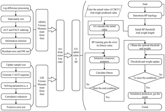
Figure 1.
Structure of the ARMA-GM-GABP combined model.
The specific implementation steps of the combined forecasting model are as follows:
- 1.
- Establish an ARMA single-term forecast model to obtain the forecast value , , ..., ) ( is the predicted value in the i-th day).
- 2.
- Establish a GM (1,1) single prediction model to obtain the predicted value , , ..., ) ( is the predicted value in the i-th day).
- 3.
- Determine the BP neural network structure according to the number of input and output parameters of the fitting function: Use the predicted value (, ), (,) …, (, ) of ARMA model and GM (1,1) model as the two-dimensional input training sample of the BP neural network (m < n), the number of input nodes is 2. Use , ,…, ) as an output target (where is the true CBCFI value at day i), the number of the output node is 1.
- 4.
- Attempt to use genetic algorithms to improve the weight and threshold of the BP neural network. First, we use the fitness function to calculate the individual fitness value, then use selection, crossover and mutation operations to determine the optimal fitness value corresponding to persons.
- 5.
- Initial weight and threshold assignment to the network using a genetic algorithm to obtain the optimal individual, and then we use the trained combination model to predict the test sample (, )…, (, ). Predict the CBCFI for the test date and compare it with the true value to test the prediction ability of the network.
3. Empirical Analysis
In this paper, we use the China Coastal Bulk Coal Freight Index from January 2014 to November 2019 as the sample. This work set the data from January 2014 to July 2019 as the training set and the data from August to October 2019 as the test set. The training set contains 2038 data and the test set contains 61 data. Then, we use November 2019 data as the forecast set to conduct a comparative analysis of forecast accuracy based on three models, the ARMA model, GM model and ARMA-GM-GABP combination model.
3.1. Data Volatility Analysis
Figure 2 depicts the trend of CBCFI in the sample range. The figure shows that the CBCFI data fluctuate greatly and there is a phenomenon of sharp rise and fall. In addition, the data show obvious fluctuation clustering characteristics, the larger changes are relatively concentrated in one period, while the smaller changes are relatively concentrated in another period.
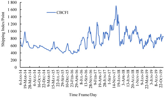
Figure 2.
Historical data of CBFI.
The large volatility of CBCFI data is mainly caused by comprehensive changes in the shipping market’s capacity and turnover in different periods. Since 2014, the growth rate of coal demand has slowed down, leading to oversupply in the charter market. The overall trend of the domestic coastal coal shipping market is sluggish, and CBCFI continues to bottom out. Coal transport prices remained low in 2015, shipping rates were able to rebound sharply in May due to a significant reduction in coal imports and a significant reduction in domestic coal prices. In December 2017, due to the accelerated pace of coal reserves in power plants in winter and the obstacles to shipping capacity in the northern region, shipping rates have jumped, reaching their highest value in recent years, which is 1706.2. The increase in hydropower squeezed coastal thermal power production in July 2019, prompting a reduction in coal consumption by high-energy-consuming enterprises, making coal pulling less active, but then, affected by typhoons and a lack of capacity supply in the market, supporting higher freight prices.
Table 1 shows the descriptive statistical characteristics of the mean, standard deviation, kurtosis and JB statistic of the CBCFI data within the sample interval. The skewness is 1.046825 > 0, the kurtosis is 4.349061 > 3 and the probability p corresponding to the JB statistic is 0, which shows that the data have a clear spike-right skew, a large deviation from the normal distribution, and a spike and fall situation.

Table 1.
Statistics characteristics of sample.
3.2. Predicting from ARMA Model
First, we establish the ARMA prediction model. It can be seen from Figure 2 that the CBCFI data fluctuate greatly in the selected sample interval, and the changing trend shows a non-stationary state. In order to eliminate the instability of the coal shipping index, we choose the daily return rate of the index as the research object. The daily return rate of the index adopts the calculation formula of the logarithmic return rate, and the daily return rate of CBCFI is expressed as:
RCBCFI = lnCBCFIt − lnCBCFIt−1
In the above formula, RCBCFI is the daily return on CBCFI after first order logarithmic differencing, CBCFIt is the daily coal freight index corresponding to day t, and CBCFIt−1 is the daily coal shipping index corresponding to day t − 1. After the first-order logarithmic difference processing, the change trend of CBCFI’s daily return is shown in Figure 3.
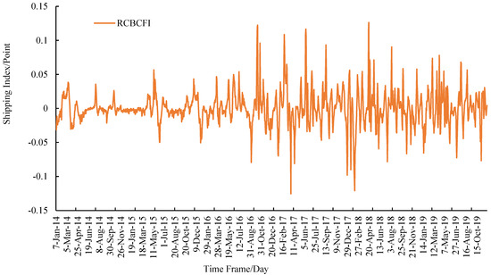
Figure 3.
Historical data of CBFI return series.
We use the ADF method to test whether RCBCFI is stationary. The T statistic is −15.97711 less than the critical value of 1% of the significance level −2.566702. The concomitant probability is 0.0000, indicating that the RCBCFI sequence does not have a unit root and is a stationary sequence, which is suitable for constructing the ARMA forecast model. By analyzing the statistical characteristics of the autocorrelation function and partial autocorrelation function, we preliminarily determine that there are two preselected models, ARMA (1,1) and ARMA (1,2).
Our work sequentially tests the two preselected models from the low level. It can be seen from the comparison of model statistics and T test results in Table 2 that the ARMA (1,2) model has passed the T test, and all indicators are overall better than the ARMA (1,1). Therefore, the ARMA (1,2) model is determined as the optimal prediction model. Then we perform an autocorrelation test on the estimated ARMA (1,2) model residuals. It is found that the autocorrelation functions of the samples are all within the 95% confidence interval, and the corresponding probability p values of the Q statistic are far greater than the test level of 0.05. Therefore, it is considered that there is no autocorrelation in the residual sequence of the model ARMA (1,2) estimation results, that is, the model construction is reasonable.
Table 2.
Parameter estimation results of ARMA model.
3.3. Predicting from GM Model
According to the modeling steps of the GM model, we first test the original CBCFI sequence for extreme ratios. The test results find that the extreme ratios of the sequence are included in the required range and meet the modeling requirements. Then we use MATLAB software to write a program and train the model to obtain the GM (1,1) model parameters , . The model prediction formula is:
To test the prediction accuracy of the above model, we use the formula C = , and to calculate the mean square error ratio C of the model, where is the difference between the original sequence and the predicted sequence; is the average of the residual sequence ; and are the standard deviations of the original series and the residual series respectively. The calculation result shows the mean squared error ratio . Then we continue to use the formula to calculate the probability of small error p = 1 > 0.95. Finally, we refer to the gray prediction accuracy test grade standard table to know that the above model has passed the test, which is the better model with level 1.
3.4. ARMA-GM-GABP Combined Model Prediction
According to the previous analysis, we use the BP neural network optimized by GA to simulate the nonlinear function. The number of nodes in the input layer is 2 and the number of nodes in the output layer is 1. In this paper, the number of hidden layer neurons affects the model fitting effect and calculation time. According to the empirical formula , the number of hidden layer neurons is preliminarily determined, where m is the number of input layer nodes, n is the number of output layer nodes and is an adjustment constant between 1–10. After calculation, it is found that is between 2 and 11. After investigating the effect of BP training with different hidden layers, we check the effect for each BP prediction result with the test group data and calculate the difference between the fitted value and the corresponding actual value. The results show that when the number of neurons is 5, the fitting effect of the neural network is better and the calculation time is shorter. Therefore, our work selects the 2-5-1 BP network prediction model. The activation function of the hidden layer is the tansig function, and the activation function of the output layer is the purelin function. The number of training times is 1000, and the error setting is 0.0001.
GA uses real number coding. Based on Equation , where is the number of neurons in the input layer, is the number of neurons in the output layer, and is the number of neurons in the hidden layer, we can calculate the length of each individual code is 21.The initial population size of the experiment is 100. We select the inverse of the BP neural network objective function as the fitness function. The selection operation uses the roulette method, the crossover operation uses the two-point arithmetic crossover method, the mutation operation uses the basic bit mutation method, and the number of iterations is 600. Finally, the 2-5-1 BP neural network with the best fit is found through iterative training and is used to predict the CBCFI values for November 2019.
3.5. Analysis of the Predicting Results
Figure 4 shows the prediction results of the ARMA model, Figure 5 shows the GM model prediction results and Figure 6 shows the prediction results of the combined model. It can be seen from the prediction fitting that the prediction result of the ARMA model can reflect the changing trend of the actual CBCFI value to a certain extent, but when the data change greatly, a big error will occur. At the same time, after an error occurs, it takes at least two units of time to correct it. For data with large fluctuations, the ARMA model will cause the predicted data to be too big or too small. The prediction of the GM model shows that it is suitable for approximating the prediction of exponential growth, so the prediction value is credible under the premise of no large data fluctuations. Therefore, the GM model is suitable for data prediction of wavelet motion. For data with large fluctuations, there is a big error between the predicted results and actual values in most cases. Through the ARMA-GM-GABP combined model, the trend of the predicted sequence is close to the actual sequence, and the correction time after an error in the forecast is no more than 1 time unit. Compared with the ARMA model and the GM model, the prediction accuracy is greatly improved.
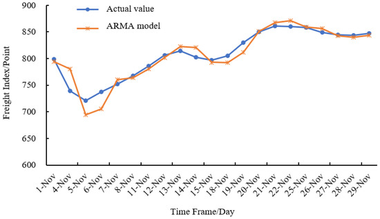
Figure 4.
Comparison between forecasting result of ARMA model and real value.
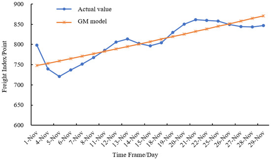
Figure 5.
Comparison between forecasting result of GM model and real value.
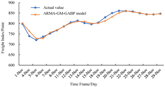
Figure 6.
Comparison between forecasting result of ARMA-GM-GABP model and real value.
In order to comprehensively assess the forecasting performance of the ARMA-GM-GABP combined model, we use the following four indicators as the assessment criteria: Mean Absolute Error (MAE), Root Mean Square Error (RMSE), Hill Inequality Coefficient (TIC) and Absolute Error (AE). MAE is used to evaluate the predictive effect of the smooth part of the CBCFI, RMES is used to evaluate the predictive effect of the high values in the CBCFI, and TIC and AE are used to evaluate the predictive power of the model and the degree of model fit. These four indicators are used to test the prediction accuracy of each model. The lower these four values, the lower the prediction error. Compared to other evaluation indicators, these four indicators can provide a more accurate assessment of the model’s prediction of the high part, the smooth part and the overall trends of the CBCFI. Therefore, it is very suitable to use these assessment indicators for evaluating the predictive effectiveness of the volatile CBCFI. The calculation formula is as follows:
In the above formula: is the predicted value of CBCFI; is the actual value of CBCFI; N is the data sample size.
The comparative analysis of predictive indicators of these three models ARMA, GM and ARMA-GM-GABP is shown in Table 3 and Figure 7. The test results show that:
- The MAE of the combined ARMA-GM-GABP forecasting model is 5.8780, a decrease of 44.16% compared to the ARMA model and 67.37% compared to the GM (1,1) model. This suggests that the ARMA-GM-GABP model has improved the prediction of the smooth part of the CBCFI series.
- The RMSE of the combined ARMA-GM-GABP forecasting model is 8.5889, a decrease of 42.25% compared to the ARMA model and 60.1% compared to the GM (1,1) model. It shows that the prediction accuracy of the high-value part of the model is then significantly improved.
- The combined ARMA-GM-GABP forecasting model has improved the predictive ability and fits of the CBCFI with a TIC of 0.0053, a decrease of 42.4% compared to the ARMA model and 60.15% compared to the GM (1,1) model. It shows that the combined ARMA-GM-GABP forecasting model has better forecasting ability compared to other models.
- From Figure 7, we can find that the AE curve of the combined model is the lowest in the vast majority of cases. There are only four instances where it is not the lowest and will correct to be the lowest within a unit of time.
Table 3.
Forecasting index of three models.
Table 3.
Forecasting index of three models.
| Predictive Model | |||
|---|---|---|---|
| ARMA | 10.5260 | 14.8729 | 0.0092 |
| GM | 18.0132 | 21.5242 | 0.0133 |
| Combined | 5.8780 | 8.5889 | 0.0053 |
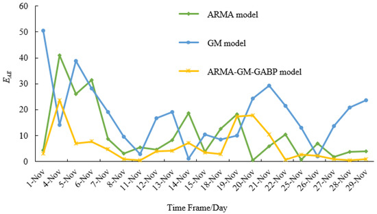
Figure 7.
EAE of three prediction models.
All of the above suggests that the ARMA-GM-GABP combined model is more suitable for CBCFI forecasting than the ARMA model and the GM (1,1) model.
4. Conclusions
In this paper, we select CBCFI as the research object. First of all, our work uses ARMA model prediction. ARMA model is the most commonly used model to deal with time series. By fitting the linear characteristics of the time series, it can often get good results. However, for the CBCFI, which is a noisy and non-smooth series, the linear analysis alone does not give a good result. Second, we use the GM (1,1) model, which is the most widely used grey dynamic prediction model in grey system theory. Only a few prediction values of this model have relatively small errors, but the other prediction values can only reflect the growth trend of the data series to a certain extent, and the prediction accuracy is relatively low.
In response to the large fluctuations in the CBCFI, which contains noise and the series itself is non-linear and non-stationary. This paper establishes a combined ARMA-GM-GABP forecasting model to forecast the CBCFI. The empirical analysis results show that the ARMA-GM-GABP combined model has the following advantages compared to traditional forecasting models:
- Effective capture of trend information.
- ARMA model can capture the periodicity and trend information of the original data series well. Therefore, using the predicted data from the ARMA model as input to the GABP model allows the combined model to more accurately predict trends of the CBCFI.
- Noise reduction.
- The GM (1,1) model allows for effective noise reduction of the original CBCFI series, providing stable input data for the GA-BP prediction model.
- Better prediction and accuracy.
- Compare to the ARMA model and GM (1,1) model, the MAE and RMESE of the combined ARMA-GM-GABP forecasting model decreased by 67.37% and 60.09%, respectively. Its prediction error is significantly smaller than that of the ARMA model and GM (1,1) model.
- General predictive applicability.
- The combined ARMA-GM-GABP forecasting model is constructed based on the CBCFI series in the years since 2014. Due to the extreme volatility of CBCFI over this time period, the ARMA-GM-GABP combined forecasting model is trained to have general predictive applicability to CBCFI over different time periods.
Above all, the ARMA-GM-GABP combined model can make up for the deficiency of the single prediction models. It has good modeling and prediction advantages for dealing with the original modeling data with volatility, periodicity and trend, so the model has good prediction performance. The ARMA-GM-GABP combined model provides scientifically accurate forecasts of the CBCFI, which can support the government and relevant departments in better macroeconomic regulation and control and enable relevant enterprises and participants in the coastal shipping market to better obtain market information and grasp market dynamics. The areas for improvement of the combined forecasting model include: (1) Optimization of single-term models ARMA and GM; (2) Considering the selection of models with better forecasting effects as single-term forecasting models. In the future, as our research progresses, we will try to improve the combined model and extend it to other shipping indices, in order to further verify the validity and practicality of the model in practical applications, and provide support for shipping market operators and investors to better grasp market trends and formulate strategies.
Author Contributions
Conceptualization, W.P. and L.W.; methodology, Z.L.; software, W.P. and L.W. and Y.F.; validation, W.P. and L.W.; formal analysis, X.W.; investigation, X.W. and Y.F.; resources, Z.L.; data curation, X.W and W.P.; writing—original draft preparation, W.P. and L.W.; writing—review and editing, Z.L. and R.F.; project administration, Y.F. All authors have read and agreed to the published version of the manuscript.
Funding
This work was funded by the National Natural Science Foundation of China under Grant 71801028, the Social Science Planning Fund of Liaoning Province Grant L18CTQ004, and China Postdoctoral Science Foundation Grant 2015M571292.
Institutional Review Board Statement
Not applicable.
Informed Consent Statement
Not applicable.
Data Availability Statement
The data presented in this study are available upon request.
Conflicts of Interest
The authors declare no conflict of interest.
References
- Tan, H.; Yang, J. An Empirical Analysis of the Correlation between China’s Coastal and Yangtze River Coal Freight Price Volatility Based on VAR. J. Wuhan Univ. Technol. 2021, 45, 161–165. [Google Scholar]
- Wang, S.; Chen, J.; Yu, S. China’s coastal and international dry bulk freight rates linkage. China Navig. 2016, 39, 114–118. [Google Scholar]
- Liu, C.; Liu, J.; Yang, J. Evaluation of Volatility of Coastal Coal Freight Index Based on ARCH Family Models. J. Wuhan Univ. Technol. 2012, 3, 445–449. [Google Scholar]
- Xiao, W.; Xu, C.; Liu, A. Hybrid LSTM-Based Ensemble Learning Approach for China Coastal Bulk Coal Freight Index Prediction. J. Adv. Transp. 2021, 2021, 5573650. [Google Scholar] [CrossRef]
- Wang, S. Analyzing the Influence of Each Influencing Factor on the Freight Rate of Coastal Coal Based on Analytic Hierarchy Process. Int. Core J. Eng. 2020, 6, 256–261. [Google Scholar]
- Chen, Y. Forecasting Baltic dry index with unequal-interval grey wave forecasting model. J. Dalian Marit. Univ. 2015, 41, 96–101. [Google Scholar]
- Liang, W.; Lu, C. Export Containerized Freight Index Estimation Model Based on Neural Network. Comput. Simul. 2013, 30, 421–425. [Google Scholar]
- Lian, Y. Crude Oil Tanker Freight Rate Forecasting Based on ARMA and Artificial Neural Network; Shanghai Jiao Tong University: Shanghai, China, 2015. [Google Scholar]
- Yuan, Y.; Wang, B. Forecast on highway logistics freight price index of China by ARIMA model. Math. Pract. Theory 2017, 47, 52–57. [Google Scholar]
- Zhou, Y.; Yang, J. A study on the fluctuation characteristics of China’s coastal container shipping index. J. Wuhan Univ. Technol. 2022, 44, 32–39. [Google Scholar]
- Adland, R.; Cullinane, K. The nonlinear dynamics of spot freight rates in tanker markets. Transp. Res. Part E Logist. Transp. Rev. 2006, 42, 211–224. [Google Scholar] [CrossRef]
- Shan, F. China Export Container Freight Index Forecast Based on Wavelet Analysis and ARIMA Model. Master’s thesis, Dalian Maritime University, Dalian, China, 2013. [Google Scholar]
- Li, C. Price Forecasting Analysis of BP Neural Network Based on Improved Genetic Algorithm. Comput. Technol. Dev. 2018, 28, 144–151. [Google Scholar]
- Wang, Y. Analysis and Forecast of Stock Price Based on ARMA Model. Product. Res. 2021, 09, 124–127. [Google Scholar]
- Xu, D.; Zhou, C.; Guan, C. Prediction method of equipment failure rate based on ARMA-BP combined model. Agriculture 2022, 12, 793. [Google Scholar]
- Wu, D.; Wu, C. Research on the Time-Dependent Split Delivery Green Vehicle Routing Problem for Fresh Agricultural Products with Multiple Time Windows. Agriculture 2022, 12, 793. [Google Scholar] [CrossRef]
- Xu, Y.; Chen, X. Comparison of Seasonal ARIMA Model and LSTM Neural Network Forecast. Stat. Decis. 2021, 37, 46–50. [Google Scholar]
- Liu, Z.; Ding, Y.; Yan, J. Frequency prediction of SVR-ARMA combined model based on particle swarm optimization. Vib. Test. Diagn. 2020, 40, 374–380. [Google Scholar]
- Wang, H. Multi-objective optimization design of ARMA control chart considering both efficiency and cost. Oper. Res. Manag. 2021, 30, 80–86. [Google Scholar]
- Chen, H.Y.; Miao, F.; Chen, Y.J.; Xiong, Y.J.; Chen, T.A. Hyperspectral image classification method using multifeature vectors and optimized KELM. IEEE J. Sel. Top. Appl. Earth Obs. Remote Sens. 2021, 14, 2781–2795. [Google Scholar] [CrossRef]
- Gao, C.; Kong, X.; Shen, X. Evaluation of Frost Resistance of Stress-damaged Lightweight Aggregate Concrete Based on GM (1,1). Eng. Sci. Technol. 2021, 53, 184–190. [Google Scholar]
- Wang, H.; Jing, W.; Zhao, G. Fatigue life prediction of hydraulic support base based on gray system model GM (1, 1) improved Miner criterion. J. Shanghai Jiao Tong Univ. 2020, 54, 106–110. [Google Scholar]
- Kang, C.; Gong, L.; Wang, Z. Predicting the deterioration of hydraulic concrete by using grey residual GM (1,1)-Markov model. J. Water Resour. Water Transp. Eng. 2021, 1, 95–103. [Google Scholar]
- Zhou, X.B.; Ma, H.J.; Gu, J.G.; Chen, H.L.; Deng, W. Parameter adaptation-based ant colony optimization with dynamic hybrid mechanism. Eng. Appl. Intell. 2022, 114, 105139. [Google Scholar] [CrossRef]
- Qian, K.; Hou, Z.; Sun, D. Sound Quality Estimation of Electric Vehicles Based on GA-BP Artificial Neural Networks. Appl. Sci. 2020, 10, 5567. [Google Scholar] [CrossRef]
- Wu, D.; Hong, N.; Yi, L.; Hui, C.; Hui, Z. An adaptive different evolution algorithm based on belief space and generalized opposition=based learning for resource allocation. Appl. Soft Comput. 2022, 127, 1568–4946. [Google Scholar]
- Chen, Y.; Hu, Y.; Zhang, S.; Mei, X.; Shi, Q. Optimized Erosion Prediction with MAGA Algorithm Based on BP Neural Network for Submerged Low-Pressure Water Jet. Appl. Sci. 2020, 10, 2926. [Google Scholar] [CrossRef]
- Zhang, G.; Zheng, Y.; Liao, K. Research on Ink Color Matching Based on GABP Algorithm. J. Xi’an Univ. Technol. 2019, 35, 113–119. [Google Scholar]
- Yao, R.; Guo, C.; Deng, W.; Zhao, H.M. A novel mathematical morphology spectrum entropy based on scale-adaptive techniques. ISA Trans. 2022, 126, 691–702. [Google Scholar] [CrossRef]
- Yu, Q.; Zhang, Z.; Qu, Y. Prediction of Lost Load of Power Grid Blackout Based on ARMA-GABP Combined Model. China Power 2018, 51, 38–44. [Google Scholar]
Publisher’s Note: MDPI stays neutral with regard to jurisdictional claims in published maps and institutional affiliations. |
© 2022 by the authors. Licensee MDPI, Basel, Switzerland. This article is an open access article distributed under the terms and conditions of the Creative Commons Attribution (CC BY) license (https://creativecommons.org/licenses/by/4.0/).