Abstract
Surface-defect detection is crucial for assuring the quality of strip-steel manufacturing. Strip-steel surface-defect detection requires defect classification and precision localization, which is a challenge in real-world applications. In this research, we propose an improved PP-YOLOE-m network for detecting strip-steel surface defects. First, data augmentation is performed to avoid the overfitting problem and to improve the model’s capacity for generalization. Secondly, Coordinate Attention is embedded in the CSPRes structure of the backbone network to improve the backbone network’s feature extraction capabilities and obtain more spatial location information. Thirdly, Spatial Pyramid Pooling is specifically replaced for the Atrous Spatial Pyramid Pooling in the neck network, enabling the multi-scale network to broaden its receptive field and gain more information globally. Finally, the SIoU loss function more accurately calculates the regression loss over GIoU. Experimental results show that the improved PP-YOLOE-m network’s AP, AP, and AP, respectively, achieved 44.6%, 80.3%, and 45.3% for strip-steel surface defects detection on the NEU-DET dataset and improved by 2.2%, 4.3%, and 4.6% over the PP-YOLOE-m network. Further, our method has fast and real-time detection capabilities and can run at 95 FPS on a single Tesla V100 GPU.
1. Introduction
The need for strip-steel has gradually increased across all sectors of society as the social economy has expanded. Yet, quality control in strip-steel manufacturing has always been a severe concern for industrial production. Many defects, including scratches, burrs, iron scales, contamination, inclusions, and bright marks, may appear during the manufacture of strip-steel due to variables including the production raw materials, rolling technique, and system control. These defects, in addition to the strip’s surface, significantly reduce the strip’s high-temperature resistance, corrosion resistance, wear resistance, and strength. As a result, improving strip-steel quality and production efficiency requires a rapid and accurate strip-steel surface-defect-detection method.
Methods for detecting early strip-steel surface defects include manual sampling, eddy current detection, magnetic flux leakage detection, infrared detection, laser scanning detection, and others [1]. The manual sampling method includes picking and detecting defect samples using the naked eye. This detection method easily fatigues inspectors and is a great test of the inspector’s dedication and level. The eddy current detection is a non-destructive testing method based on electromagnetic induction theory. When detecting large areas, the detecting speed cannot meet the demands of high-speed strip-steel manufacturing lines.
The magnetic flux leakage detection is limited in the types of defects, and it is unsuitable for faults with minor flaws. Due to infrared’s limited capacity for absorption, the accurate classification of defect categories is not possible using infrared detection technology for strip defects. The laser scanning detection method dramatically reduces the effectiveness and applicability of this method because the dust and substances on the production line will affect the reflection of light.
At the end of the 20th century, due to the rapid development of CCD technology, conventional machine-vision-detection methods made tremendous strides in recognizing strip defects. Traditional machine-vision-detection methods have a number of benefits over earlier detection methods, including improved dependability, increased efficiency, and enhanced practicability. This detection approach still necessitates manual feature extraction, which is detrimental to boosting industrial production efficiency and industry automation.
Deep learning has advanced quickly in recent decades, with applications ranging from autonomous driving to image identification, natural language processing, intelligent predictions, and so on. To fully automate industrial quality detection, deep learning technology solutions are progressively being implemented in strip surface-defect detection.
The use of convolutional neural networks (CNN) to extract defective features for classification produced good results [2,3,4,5]; however, defect location remained a challenge. There are two types of object detection algorithms: one-stage and two-stage algorithms. The one-stage algorithms are represented by the you only look once (YOLO) series of algorithms, single shot multiBox detector (SSD), RetinaNet, etc. The two-stage algorithms are represented by Fast Region-CNN (Fast R-CNN), Faster R-CNN, Mask R-CNN, Cascade R-CNN, etc.
The one-stage algorithms conduct unified classification and regression directly and do not produce regional recommendations. This type of algorithm has low accuracy but outperforms the two-stage algorithm in terms of the detection speed. The two-stage algorithms generate some region proposals before classification and regression. This algorithm has high accuracy; however, the detection speed is slow. Many academics have undertaken successful studies on strip-steel surface defect recognition using algorithms, such as YOLO [6], SSD [7], YOLOv3 [8], RetinaNet [9], and Faster R-CNN [10,11,12].
On the basis of the aforementioned theoretical foundation, the NEU-DET dataset is used as the study object in this paper, and a network that is based on an improved PP-YOLOE-m is proposed in order to perform rapid and accurate recognition of surface defects in strip-steel.
In a nutshell, the following are the four most significant contributions in this paper:
- We employ an automated data augmentation strategy to solve the issue of overfitting during model training when the NEU-DET dataset is insufficient;
- To boost the feature extraction capability of the backbone network, we embed coordinate attention in the CSPRes structure of the backbone network;
- To enhance multi-scale fusion and expand the receptive field, we replace the Spatial Pyramid Pooling module with the Atrous Spatial Pyramid Pooling in the CSPBlock structure of the neck network;
- The GIoU loss function does not take into consideration the distance, aspect ratio, and angle between two box factors. Therefore, we use the SIoU loss function, which does.
The remainder of this paper is divided into the following sections. Related work study on strip surface-defect detection is introduced in Section 2. PP-YOLOE algorithm, and its improvements are thoroughly depicted in Section 3. The experimental implementation details, evaluation metrics, ablation experiments, and experimental results are described in Section 4. Our conclusions and recommendations for further study are provided in Section 5.
2. Related Work
There are currently two primary approaches to strip surface-defect detection based on machine vision. These approaches are divided into two categories: tradition and deep learning.
2.1. Traditional Strip-Steel Surface-Detection Approaches
Traditional approaches for detecting strip-steel surface defects based on machine vision may be divided into three main categories: those that are based on local anomaly [13,14,15,16], those that use template matching [17,18,19,20,21], and those that use machine learning [22,23,24,25].
(1) Local anomaly: The texture of the picture under test is analyzed in order to detect normal behavior that does not adhere to an explicit definition. In the space domain, one-stage and two-stage statistical approaches, such as the covariance matrix [13], the weighted covariance matrix [14] and the Weibull model [15,16], are used. In the frequency domain, the spectrum features are extracted by means of wavelet and Fourier transforms.
(2) Template matching: Defect detection is achieved by conducting location operations on the defect-free template image and the image to be examined, such as similarity computation or image registration. During detection, the approaches are readily influenced by the imaging environment, and the spatial location, light qualities, and geometric properties of objects in the picture will also change significantly.
(3) Machine learning: The procedure consists of image processing, feature extraction, and defect classification using models. Typical classifiers consist of SVM, K-nearest neighbor, and decision tree, among others. Numerous scholars have also improved the detection performance of the strip-steel surface-defect detection classifier by studying and bolstering the classifier’s performance [22,23,24,25].
The aforementioned approaches necessitate substantial professional knowledge, require hand-crafted extracting features, are susceptible to environmental influences, and are not conducive to complete industrial automation.
2.2. Strip-Steel Surface-Detection Approaches of Deep Learning
In deep learning, strip-steel surface-defect detection is possible using three approaches: object detection, semantic segmentation, and GAN.
(1) Object detection: Li et al. [6] proposed an end-to-end detection approach based on improved YOLO, including 27 convolutional layers in the improved network. Lin et al. [7] proposed an improved SSD detector for defect localization and a ResNet50 network for defect classification.
Zhang et al. [8] proposed a CP-YOLOv3-dense detection approach that preferentially uses convolutional networks to classify pictures and then locates defects. Cheng et al. [9] proposed a deep neural network for differential channel attention and adaptive spatial feature fusion based on the RetinaNet detection network. Refs. [6,7,8,9] used the one-stage algorithm, which has significant speed benefits; however, the two-stage algorithm’s precision is better. In [6], the approach is less feasible.
Refs. [7,8] separated the work of defect localization and classification into two phases in the defect detection process, which costs greater detection time. In [8], the classification priority concept was applied to a single image with a single defect but not to a single image with multiple defects. In [9], adaptive feature fusion resulted in an increase in the computation and model parameters, as well as a prolonged in the model inference process. In [10,11,12], these approaches are all based on the Faster R-CNN architecture.
He et al. [10] proposed two distinct deep networks as convolutional layers, ResNet34 and ResNet50, to generate multi-level features from convolutional neural networks and fuse them into one feature. Ren et al. [11] substitutes the backbone network VGG’s convolution with a depthwise separable convolution and introduces center loss. Tang et al. [12] adopted Resnet50 as the backbone network, while also introducing the attention and MSMP module. These approaches of two-stage [10,11,12] are extremely precise in detecting strip defects; however, they do not fulfill the actual manufacturing process speed requirements.
(2) Semantic segmentation: Praveen et al. [26] explored two encoders, ResNet and DenseNet, based on U-Net on the Severstal dataset, employing migration learning to obtain excellent results in classification and segmentation tasks. Dong et al. [27] proposed a pixel-level surface-defect detection system based on pyramid feature fusion and global context attention network (PGA-Net), which was experimentally validated on several defect datasets and yielded great results. Bao et al. [28] proposed a novel TGRNet network that employs triple to segment defect and background areas and multi-graph reasoning to explore the similarity between different images. These approaches are all pixel-level defect detection methods, which are more accurate for defect identification and location. Still, the training and inference process takes longer than the object detection method.
(3) GAN: Liu et al. [29] proposed a GAN-based strip-steel surface-defect detection approach that uses the GAN generator’s second to last output layer as the feature layer and normal samples to conduct single-class classification by comparing the characteristics of normal and abnormal samples. This approach can perform unsupervised learning on a limited number of samples; however, it can only categorize single-class flaws and cannot locate defects.
The deep learning methodology has a significant benefit over traditional strip surface-defect detection approaches in that the extraction is automated, thereby, eliminating the need to extract features manually. Manual feature extraction is a time-consuming and challenging task that demands high-level expertise. The above-mentioned algorithms for object detection are anchor-based, and the detection accuracy is dependent on the initial anchor setting. This paper proposes an improved method based on the PP-YOLOE-m anchor-free paradigm detection network, which addresses the slow detection speed and dependence on anchor settings and guarantees high-precision detection results.
3. Methods
3.1. PP-YOLOE Algorithm
The PP-YOLOE algorithm [30] is described in detail in three aspects: network structure, sample matching, and loss function.
3.1.1. PP-YOLOE-m Network Structure
The PP-YOLOE-m network structure is divided into three sections: backbone, neck, and head. Backbone uses the CSPResNet network to extract defect features, and its internal structure comprises mainly CBS, RepVGG Block, Res Block, EffectiveSE, CSPRes, and so on. Neck employs the PANet structure for multi-scale fusion, which is a top-down and bottom-up bi-directional feature pyramid. Head completes the defect classification and regression tasks. Figure 1 shows the PP-YOLOE-m network structure as well as core module components. In the backbone of Figure 1, the first parameter denotes the change in the number of channels, while the second parameter represents the number of Res Blocks in the CSPRes structure.

Figure 1.
The PP-YOLOE-m network structure.
3.1.2. Sample Matching
PP-YOLOE is an anchor-free algorithm that matches samples employing Adaptive Training Sample Selection (ATSS) and Task Alignment Learning (TAL). ATSS selects appropriate anchors as positive samples based on the correlation statistic characteristics of ground truth (gt), and TAL and then calculates the degree of task alignment for each anchor. The loss of task alignment might progressively unite the optimal anchor for classification and location. The ATSS calculation process is shown in Algorithm 1, and the TAL calculation process is shown in Algorithm 2.
| Algorithm 1 Adaptive Training Sample Selection Algorithm |
|
| Algorithm 2 Task Alignment Learning Algorithm |
|
3.1.3. Loss Function
The PP-YOLOE algorithm’s total loss is composed of three components: classification loss, regression loss, and DF loss, which may be expressed as:
where a, b, and c denote weight coefficient.
The classification loss is improved via the asymmetric treatment of positive and negative data and the construction of a new classification loss function based on Focal Loss:
where denotes positive and negative sample weight, denotes an adjustable factor, p denotes the predicted IoU-aware classification score, and q denotes the object IoU score.
The box regression loss is computed by the GIoU loss function:
where C denotes the smallest external rectangular box of A and B.
Since the actual distribution is usually not far from the labeled locations, to allow the network to focus quickly on areas near the label, PP-YOLOE adds an additional DF loss, which is calculated as follows:
where y denotes the labeled dot, and denote closed dots, and and denote the output node.
3.2. Data Augmentation
Due to the limited number of NEU-DET datasets, we employed an automatically learned data augmentation (Autoaugment) strategy [31] to prevent model overfitting. This strategy defines 22 data processing operations, the majority of which are color, geometry transformation, and bounding box. The data augmentation strategy is divided into 20 sub-strategies, each with two data operations. Each operation defines two hyperparameters: probability P and intensity M, which will be discretized into six equal intervals. Finding a sub-policy entails searching in a discrete space of size , while the overall search space is .
The cost of searching for a sub-strategy is high due to a large number of possibilities in the search space, and a Proximal Policy Optimization (PPO) method is utilized for the search. The PPO calculation process is shown in Algorithm 3, and the data augmentation operation details are depicted in Table 1.
| Algorithm 3 Proximal Policy Optimization Algorithm (adapted from [32]) |
|

Table 1.
Examples of learned augmentation sub-strategies. Each operation in an augmentation sub-strategy is represented by a triplet: the operation, its likelihood of being used, and its magnitude.
3.3. Improved PP-YOLOE-m Network Structure
The PP-YOLOE-m network structure is improved in two ways in this paper: the attention mechanism is embedded in the backbone network’s CSPRes module, and the SPP is replaced with ASPP in the neck network’s first CSPBlock module. The improved PP-YOLOE-m network structure is shown in Figure 2. These two parts for improvements are discussed in depth in the following sections.
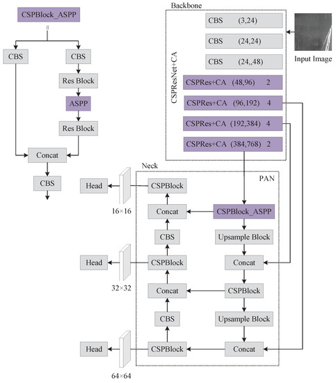
Figure 2.
The improved PP-YOLOE-m network structure.
3.3.1. Coordinate Attention
Since the backbone network can only extract local relationships and the feature extraction ability is limited with the network depth, we emploedy a Coordinate Attention [33] that considers direction-related location information in addition to channel information, thereby, allowing the model to better localize and identify defects. We embed the coordinate attention into the Res Block module of the backbone network, and the specific embedding position of the coordinate attention is shown in Figure 3.
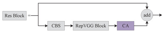
Figure 3.
Embedding coordinate attention to the Res Block.
The Coordinate Attention encodes channel and distant dependencies with accurate location information. Coordinate information embedding and attention generation, which are represented in Figure 4, are two processes that make up coordinated attention. It is more difficult to preserve location information with the global pooling strategy since it compresses spatial data globally into channels. Global pooling is converted into two one-dimensional feature encodings so that the attention module may capture long-distance spatial relationships with precise location information.
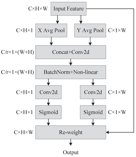
Figure 4.
Coordinate attention generation process.
Given an input , each channel is encoded with one dimension and along the horizontal and vertical axes, respectively. Hence, the expression for the output of the c-th channel with height h is:
Likewise, the output of the c-th channel of width w is expressed as:
The aggregated feature maps from Equations (6) and (7) are concatenated. The concatenated feature subsequently was placed in a common convolutional transform function to find:
where denotes the concatenation operation, is a activation function and is an intermediate feature mapping that encodes spatial information in the horizontal and vertical directions. Along the spatial dimension, is separated into two distinct tensors and . Utilizing two convolutions, and , and are converted into two tensors with the same number of input channels. The equation can be formulated as follows:
where is the sigmoid activation function. After that, and are expanded, and then, accordingly, they are employed as attention weights. The coordinate attention module’s output is:
3.3.2. Atrous Spatial Pyramid Pooling
Spatial Pyramid Pooling (SPP) is capable of extracting information from different receptive fields but does not adequately capture the semantic relations in global and local contexts. Atrous Spatial Pyramid Pooling (ASPP) [34] can enlarge the network’s receptive field without downsampling and improve the network’s ability to obtain multiscale contextual information. In actuality, the PP-YOLOE-m network utilizes SPP only in the first CSPBlock module of the multiscale structured PANet but not in the other CSPBlocks.
Thus, we replaced the SPP module in the first CSPBlock module of the multiscale structured PANet with the ASPP module. We applied various rate expansion factors to complete convolution operations to the input feature, concatenate several feature maps and feature maps of pooling the input feature, and finally, output fused feature using convolution. Figure 5 depicts the SPP and ASPP work pross.

Figure 5.
Network structure of two pooling ways. (a) Spatial Pyramid Pooling (SPP). (b) Atrous Spatial Pyramid Pooling (ASPP).
3.4. SIoU Loss Function
The GIoU loss function is used in the bounding box regression loss computation of the PP-YOLOE. On the basis of IoU, GIoU proposed the notion of the minimal circumscribed rectangle of the ground truth and the prediction bounding box of it to solve the problem of the two bounding boxes not intersecting. GIoU, on the other hand, ignores the distance, aspect ratio, and angle between the two bounding boxes. We employed the SIoU loss function [35] that takes the aforementioned aspects into consideration.
The SIoU loss function has four components: angle cost, distance cost, shape cost, and IoU cost. Angle loss is accomplished by reducing the values of distance-related variables, which is referred to as the angle-aware LF component. To achieve this, the accomplishment process will first attempt to minimize if and otherwise minimize . The angle coast contribution is shown in Figure 6a. The LF component is defined as follows:
where
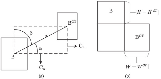
Figure 6.
Ground truth and bounding box relationship diagram. (a) The scheme for calculating the loss function’s angle cost contribution. (b) The scheme of the relation of the IoU component contribution.
The angle loss is mostly used to aid in the calculation of the distance between the two bounding boxes, and the distance cost is defined as:
where
As , the contribution to the total loss decreases; however, as , the contribution to the overall loss increases. The shape cost of the form between the two bounding boxes is defined as:
where
and denotes the shape costs. The overlapping area loss is the IoU loss, and thus the total loss is calculated as follows:
where
4. Results
The validity of the improved PP-YOLOE was experimentally validated using the NEU-DET dataset [17], which is classified into six defect categories: crazing (Cr), inclusion (In), patches (Pa), rolled-in scale (RS), pitted surface (Ps), and scratches (Sc). Each defect category has 300 grayscale images of size , for a total of 1800 images.
4.1. Implementation Details
(1) Computation Platform: We ran our method in a NVIDIA Tesla V100 GPU (with 16G memory), CUDA 11.2, and cuDNN 7.6 on Ubuntu 16.04. Our method was implemented with an end-to-end PaddleDetection Suite.
(2) Parameter Setting:The PP-YOLOE algorithm includes four network architectures with varying widths and depths, PP-YOLOE-s, PP-YOLOE-m, PP-YOLO-l, and PP-YOLO-x. We tested each of PP-YOLOE’s networks and found that PP-YOLOE-m performed the best.
As a result, we chose PP-YOLOE-m as the baseline experiment, and all of the improvement trials in this study are based on it. During the training process, the input image be resized to , the CSPResNet backbone network be loaded with weights that had already been trained with the COCO2017 dataset, the network parameters are iteratively updated using the Momentum method with the initial momentum parameter set to 0.9, the initial learning rate set to 0.0035, the batch size set to 12, the trained epochs set to 300, and the model saved once every 10 epochs.
4.2. Defect Detection on NEU-DET
The NEU-DET dataset was divided into the training set and test set in an 8:2 ratio. 1440 pictures were fed to the network for training, and 360 pictures were used for testing the model. In terms of data augmentation, we attempted many tactics, including GridMask, Mixup, Mosaic, and AutoAugment; however, only AutoAugment was successful. In terms of network structure improvement, we attempted to add an additional detecting head; however, the experimental results were unsatisfactory.
We attemptted to embed Coordinate Attention in various network locations with some success in the backbone network and the Neck. When we utilized ASPP pooling instead of SPP, we found that employing Coordinate Attention on PANet performed worse than not using it. Thus, we no longer embed coordinated attention in PANet. For the loss function, we used EIoU and SIoU loss functions, and SIoU outperformed EIoU in the experiment, which is the reason why we chose SIoU. Finally, we also conduct ablation experiments and compare the results of our improved approach to those of the most prevalent major object detection algorithms currently being used.
The Average Precision (AP) is used as an evaluation metric of experimental findings in this research. AP considers both precision and recall metrics. Precision and recall are defined as follows:
where denotes the bounding box numbers of , denotes the bounding box numbers of , and denotes the ground truth that is not detected. For a continuous precision and recall relationship curve, AP is defined as follows:
In this paper, AP signifies the AP mean value of 0.5:0.05:0.95, AP signifies the AP value of , AP signifies the AP value of , AP signifies the AP value of 0.5:0.05:0.95 and for small objects, AP signifies the AP value of 0.5:0.05:0.95 and for medium objects, and AP signifies the AP value of 0.5:0.05:0.95 a and for large objects.
Figure 7 shows the comparison of the results before and after data augmentation of the PP-YOLOE-m network. When data augmentation is used, the AP obviously improves by 1.7%. According to the AP evaluation metrics, data augmentation does not boost the effectiveness of small object recognition. The AP evaluation metrics show a significant improvement in detection precision for large objects, with a 2.8% improvement. With the exception of AP, all indicators improved to varying degrees when the data augmentation was implemented.
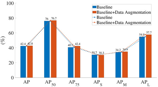
Figure 7.
Comparison of the results before and after data augmentation.
Figure 8 shows a comparison of the heat map visualization results of the baseline experiment and embedding the Coordinate Attention’s network. The baseline network on the crazing (Cr) category defect did not concentrate on the defective region, and the embedding of Coordinate Attention was significantly improved. With the embedding of the Coordinate Attention, attention was primarily focused on areas with inclusion (In) category flaws rather than on extra regions with no faults as it had been in the baseline experiment.
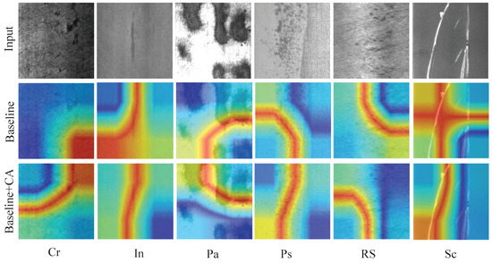
Figure 8.
Comparison of the heat map visualization results before and after embedding Coordinate Attention.
On pitted surface (Ps) category defects, the embedding of Coordinate Attention focuses on the faulty area was more comprehensive than the baseline experiment’s focus on the defective region. The area of attention after embedding the Coordinate Attention was also better than the baseline experiment on patches (Pa), rolled-in scale (RS), and scratches (Sc) category defects. The experimental results show that the embedding Coordinate Attention strengthens the defect feature extraction capability of the backbone network and can obtain more defect location information.
We set up three separate sets of parameters for comparative studies in order to assess the influence of different rate expansion factors of ASPP modules on detection results. To avoid the impact of variable rate expansion factors on the detection results, this study directly replaced the SPP module with the ASPP module with varied rate expansion factors for experiments based on the baseline model. A large expansion factor step, as illustrated in Table 2, is not as beneficial for detection precision as a small expansion factor step. When we increased the small step size by one more expansion factor, this had the opposite effect of improving detection. Thus, we chose (1,6,12,18) as the expansion factors of ASPP.
Table 2.
Comparison of different rates in the ASPP module.
Figure 9 depicts the monitoring of critical SIoU and GIoU indicators in the training of the 200 epochs. In the around 150th epoch, the SIoU loss function’s AP, AP, and AP eventually surpasses the GIoU loss function. However, the SIoU loss function does not outperform GIoU loss function in Average Recall (AR) metrics. There, AR signifies the mean AR value of 0.5:0.05:0.95.
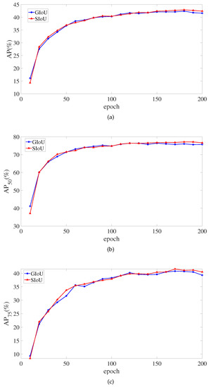

Figure 9.
The AP and AR value changes during training. (a) The change curves of the AP value. (b) The change curves of the AP value. (c) The change curves of the AP value. (d) The change curves of the AR value.
To verify the validity of the improvement on the baseline PP-YOLOE-m network, ablation experiments were conducted on the NEU-DET dataset in this paper. For each of the improvements in the baseline model PP-YOLOE-m, separate experiments were conducted, and from Table 3, it can be seen that each improvement point improved the detection precision from the original. In particular, the average accuracy improvement is most obvious when the SPP module is replaced by the ASPP module, and AP, AP, and AP improved by 1.3%, 2.5%, and 1.6%, respectively.
Table 3.
Ablation study with different component combinations on the NEU-DET dataset.
The ASPP pooling approach expands the receptive fields and obtains more global information on strip defects. AP, AP, and AP are further improved by using the SIoU loss function based on the data enhancement. Embedding CA attention mechanism and the ASPP module replacing the SPP module are improvements belonging to the network structure, and we conducted experiments on the combination of these two.The average precision was better than the results of the experiments conducted separately, and the AP substantially improved.
The CA attention mechanism captures more information and enhances the backbone network for strip defect feature extraction ability. We conducted experiments with data augmentation and using SIoU loss function based on the improved network structure, respectively, and the average precision was improved to an extent.
Table 4 shows the detection results of the current mainstream algorithms on NEU-DET data. The improved PP-YOLOE-m has the best detection precision, with AP, AP, and AP reaching 44.6%, 80.3%, 45.3%, respectively. In terms of speed, it is slightly slower than the original PP-YOLOE-m. Compared with YOLOv4, the best performing one-stage algorithm on the NEU-DET dataset, AP, AP, and AP improved by 6.8%, 8%, and 10%, respectively.
Table 4.
Detection results with other methods on the NEU-DET dataset.
AP, AP, and AP, respectively, improved by 6.5%, 7.7% and 9.1% compared to the best performing Cascade R-CNN in the two-stage algorithm. The above algorithms are anchor-based; however, this paper’s algorithm is based on anchor-free, which does not depend on the anchor setting.
4.3. Defect Result
Figure 10 shows how the algorithm in this paper tracks changes in each significant indicator while it is being trained. It is clear that, at about the 150th epoch, the values of AP begin to converge. The loss value rapidly decreases, revealing that the model fits fast.
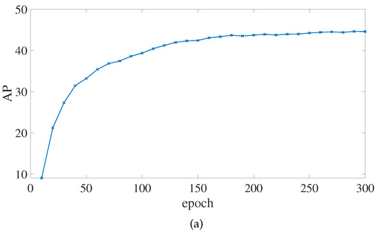

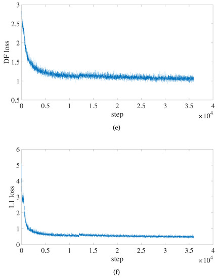
Figure 10.
AP and loss values change of the improved PP-YOLOE-m network during training. (a) The change curve of the AP value. (b) The change curve of the toatl loss value. (c) The change curve of the classification loss value. (d) The change curve of the regression loss value. (e) The change curve of the DF loss value. (f) The change curve of the L1 loss value.
Figure 11 shows the comparison of the detection results between the algorithm in this paper and PP-YOLOE-m. This paper method detects the defects above, whereas PP-YOLOE-m detects the defects below in the category of crazing (Cr) defects. While our method does not detect overlapping regions and achieves accurate location of defects, PP-YOLOE-m discovers a significant number of overlapping defect areas in the inclusion (In) and scratches (Sc) defect categories.
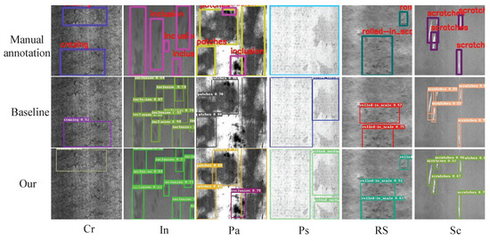
Figure 11.
The detection results of the PP-YOLOE-m and improved PP-YOLOE-m networks on the NEU-DET dataset.
There are two sorts of defects in patches (Pa); PP-YOLOE-m only picks up a single category defect; however, our approach detects the defect of the second kind. Our approach is able to identify small object defects in the pitted surface (Ps) and rolled-in scale (RS) defect categories when PP-YOLOE-m is unable to do so. The experiment results show that the algorithm in this paper has better detection and more accurate defect localization.
5. Conclusions
For the purpose of detecting strip surface defects, an improved PP-YOLOE-m network was proposed in this paper. With AP, AP, and AP reaching 44.6%, 80.3%, and 45.3%, respectively, the improved PP-YOLOE-m had the best detection precision in this paper.
The network had stronger feature extraction capability, larger receptive fields, and more accurate bounding box regression. In specific, the ASPP pooling strategy contributed to the strip’s defect detection average precision improvement, which increased by 1.3%, 2.5%, and 1.6%, respectively, for Ap, AP, and AP. On a single Tesla v100 GPU, the improved network in this paper reached 95 FPS detection performance and rapidly identified surface defects on strip steel.
The approach in this paper is based on the anchor-free method, which does not need to consider the optimization of the anchor frame and which reduces the hyperparameters, while earlier studies mostly used anchor-based networks. The following work is necessary for future research to enlarge the number of sample defect samples utilizing GAN regarding the phenomenon that insufficient samples are prone to overfitting. Additionally, knowledge distillation is an interesting approach to raising a model’s accuracy.
Author Contributions
Conceptualization, Y.Z. and X.L.; methodology, Y.Z.; software, Y.Z.; validation, Y.Z., J.G. and P.Z.; formal analysis, J.G.; investigation, P.Z.; resources, Y.Z.; data curation, P.Z.; writing—original draft preparation, Y.Z.; writing—review and editing, Y.Z., X.L. and J.G.; visualization, J.G.; supervision, X.L.; project administration, X.L.; funding acquisition, X.L. All authors have read and agreed to the published version of the manuscript.
Funding
This research was supported in part by the Science and Technology Department Project of Sichuan Provincial of China, under Grant 2017GZ0303, in part by Special Fund for Training High Level Innovative Talents of Sichuan University of Science and Engineering, under Grant B12402005, and Sichuan University of Science and Engineering for Talent introduction project, under Grant 2021RC16, and in part by University-Industry Cooperation Collaborative Education Project of the Higher Education Department of the Ministry of Education, under Grant 202101038016.
Data Availability Statement
The data that support the findings of this research are openly available at http://faculty.neu.edu.cn/songkechen/zh_CN/zhym/263269/list/index.htm (accessed on 25 June 2022).
Conflicts of Interest
The authors declare no conflict of interest.
References
- Mi, C.; Lu, K.; Wang, W.; Wang, B. Research Progress on Hot-rolled Strip Surface Defect Detection Based on Machine Vision. J. Anhui Univ. Technol. (Nat. Sci.) 2022, 39, 180–188. Available online: https://kns.cnki.net/kcms/detail/detail.aspx?FileName=HDYX202202009&DbName=CJFQ2022 (accessed on 27 May 2022).
- Yi, L.; Li, G.; Jiang, M. An end-to-end steel strip surface defects recognition system based on convolutional neural networks. Steel Res. Int. 2017, 88, 1600068. [Google Scholar] [CrossRef]
- Vannocci, M.; Ritacco, A.; Castellano, A.; Galli, F.; Vannucci, M.; Iannino, V.; Colla, V. Flatness defect detection and classification in hot rolled steel strips using convolutional neural networks. In Advances in Computational Intelligence; Rojas, I., Joya, G., Catala, A., Eds.; Springer International Publishing: Cham, Germany, 2019; pp. 220–234. [Google Scholar] [CrossRef]
- Feng, X.; Gao, X.; Luo, L. X-SDD: A new benchmark for hot rolled steel strip surface defects detection. Symmetry 2021, 13, 706. [Google Scholar] [CrossRef]
- Konovalenko, I.; Maruschak, P.; Brevus, V. Steel surface-defect detection using an ensemble of deep residual neural networks. J. Comput. Inf. Sci. Eng. 2022, 014501. [Google Scholar] [CrossRef]
- Li, J.; Su, Z.; Geng, J.; Yin, Y. Real-time detection of steel strip surface defects based on improved yolo detection network. IFAC-PapersOnLine 2018, 51, 76–81. [Google Scholar] [CrossRef]
- Lin, C.Y.; Chen, C.H.; Yang, C.Y.; Akhyar, F.; Hsu, C.Y.; Ng, H.F. Cascading convolutional neural network for steel surface defect detection. In Advances in Artificial Intelligence, Software and Systems Engineering; Ahram, T., Ed.; Springer International Publishing: Cham, Germany, 2020; pp. 202–212. [Google Scholar] [CrossRef]
- Zhang, J.; Kang, X.; Ni, H.; Ren, F. Surface-defect detection of steel strips based on classification priority YOLOv3-dense network. Ironmak. Steelmak. 2021, 48, 547–558. [Google Scholar] [CrossRef]
- Cheng, X.; Yu, J. RetinaNet with difference channel attention and adaptively spatial feature fusion for steel surface-defect detection. IEEE Trans. Instrum. Meas. 2020, 70, 2503911. [Google Scholar] [CrossRef]
- He, Y.; Song, K.; Meng, Q.; Yan, Y. An end-to-end steel surface-defect detection approach via fusing multiple hierarchical features. IEEE Trans. Instrum. Meas. 2019, 69, 1493–1504. [Google Scholar] [CrossRef]
- Ren, Q.; Geng, J.; Li, J. Slighter Faster R-CNN for real-time detection of steel strip surface defects. In Proceedings of the 2018 Chinese Automation Congress (CAC), Xi’an, China, 30 November–2 December 2018; pp. 2173–2178. [Google Scholar] [CrossRef]
- Tang, M.; Li, Y.; Yao, W.; Hou, L.; Sun, Q.; Chen, J. A strip-steel surface-defect detection method based on attention mechanism and multi-scale maxpooling. Meas. Sci. Technol. 2021, 32, 115401. [Google Scholar] [CrossRef]
- Luo, Q.; He, Y. A cost-effective and automatic surface defect inspection system for hot-rolled flat steel. Robot. Comput.-Integr. Manuf. 2016, 38, 16–30. [Google Scholar] [CrossRef]
- Tsai, D.M.; Chen, M.C.; Li, W.C.; Chiu, W.Y. A fast regularity measure for surface-defect detection. Mach. Vis. Appl. 2012, 23, 869–886. [Google Scholar] [CrossRef]
- Timm, F.; Barth, E. Non-parametric texture defect detection using Weibull features. Proc. SPIE Int. Soc. Opt. Eng. 2011, 7877, 78770J. [Google Scholar] [CrossRef]
- Liu, K.; Wang, H.; Chen, H.; Qu, E.; Tian, Y.; Sun, H. Steel surface-defect detection using a new Haar–Weibull-variance model in unsupervised manner. IEEE Trans. Instrum. Meas. 2017, 66, 2585–2596. [Google Scholar] [CrossRef]
- Song, K.; Yan, Y. A noise robust method based on completed local binary patterns for hot-rolled steel strip surface defects. Appl. Surf. Sci. 2013, 285, 858–864. [Google Scholar] [CrossRef]
- Wang, H.; Zhang, J.; Tian, Y.; Chen, H.; Sun, H.; Liu, K. A simple guidance template-based defect detection method for strip steel surfaces. IEEE Trans. Ind. Inform. 2018, 15, 2798–2809. [Google Scholar] [CrossRef]
- Luo, Q.; Sun, Y.; Li, P.; Simpson, O.; Tian, L.; He, Y. Generalized completed local binary patterns for time-efficient steel surface defect classification. IEEE Trans. Instrum. Meas. 2018, 68, 667–679. [Google Scholar] [CrossRef]
- Liu, K.; Luo, N.; Li, A.; Tian, Y.; Sajid, H.; Chen, H. A new self-reference image decomposition algorithm for strip-steel surface-defect detection. IEEE Trans. Instrum. Meas. 2019, 69, 4732–4741. [Google Scholar] [CrossRef]
- Zhang, J.; Wang, H.; Tian, Y.; Liu, K. An accurate fuzzy measure-based detection method for various types of defects on strip-steel surfaces. Comput. Ind. 2020, 122, 103231. [Google Scholar] [CrossRef]
- Xiang, Y.; Chen, L.; Zhang, X. Research on Recognition of Strip-Steel Surface Defect Based on Support Vector Machine. Ind. Control Comput. 2012, 25, 99–101. Available online: https://kns.cnki.net/kcms/detail/detail.aspx?FileName=GYKJ201208045&DbName=CJFQ2012 (accessed on 25 June 2022).
- Guo, H.; Xu, W.; Liu, Y. Steel Plate Surface Defect Recognition Based on Support Vector Machine. J. Donghua Univ. (Nat. Sci.) 2018, 44, 635–639. Available online: https://kns.cnki.net/kcms/detail/detail.aspx?FileName=DHDZ201804021&DbName=CJFQ2018 (accessed on 25 June 2022).
- Hu, H.; Liu, Y.; Liu, M.; Nie, L. Surface defect classification in large-scale strip-steel image collection via hybrid chromosome genetic algorithm. Neurocomputing 2016, 181, 86–95. [Google Scholar] [CrossRef]
- Liu, Q.; Tang, B.; Kong, J.; Wang, X. SVM Classification of Surface Defect Images of Strip Based on Multi-scale LBP Features. Modul. Mach. Tool Autom. Manuf. Tech. 2020, 27–30. Available online: http://qikan.cmes.org/zhjc/EN/10.13462/j.cnki.mmtamt.2020.12.007 (accessed on 25 June 2022).
- Damacharla, P.; Rao, A.; Ringenberg, J.; Javaid, A.Y. TLU-net: A deep learning approach for automatic steel surface defect detection. In Proceedings of the 2021 International Conference on Applied Artificial Intelligence (ICAPAI), Suzhou, China, 15–17 October 2021; pp. 1–6. [Google Scholar] [CrossRef]
- Dong, H.; Song, K.; He, Y.; Xu, J.; Yan, Y.; Meng, Q. PGA-Net: Pyramid feature fusion and global context attention network for automated surface-defect detection. IEEE Trans. Ind. Inform. 2019, 16, 7448–7458. [Google Scholar] [CrossRef]
- Bao, Y.; Song, K.; Liu, J.; Wang, Y.; Yan, Y.; Yu, H.; Li, X. Triplet-graph reasoning network for few-shot metal generic surface defect segmentation. IEEE Trans. Instrum. Meas. 2021, 70, 5011111. [Google Scholar] [CrossRef]
- Liu, K.; Li, A.; Wen, X.; Chen, H.; Yang, P. Steel surface-defect detection using GAN and one-class classifier. In Proceedings of the 2019 25th International Conference on Automation and Computing (ICAC), Lancaster, UK, 5–7 September 2019; pp. 1–6. [Google Scholar] [CrossRef]
- Xu, S.; Wang, X.; Lv, W.; Chang, Q.; Cui, C.; Deng, K.; Wang, G.; Dang, Q.; Wei, S.; Du, Y.; et al. PP-YOLOE: An evolved version of YOLO. arXiv 2022, arXiv:2203.16250. [Google Scholar]
- Zoph, B.; Cubuk, E.D.; Ghiasi, G.; Lin, T.Y.; Shlens, J.; Le, Q.V. Learning data augmentation strategies for object detection. In Proceedings of the European Conference on Computer Vision, Online, 23–28 August 2020; pp. 566–583. [Google Scholar] [CrossRef]
- Heess, N.; TB, D.; Sriram, S.; Lemmon, J.; Merel, J.; Wayne, G.; Tassa, Y.; Erez, T.; Wang, Z.; Eslami, S.; et al. Emergence of locomotion behaviours in rich environments. arXiv 2017, arXiv:1707.02286. [Google Scholar]
- Hou, Q.; Zhou, D.; Feng, J. Coordinate attention for efficient mobile network design. In Proceedings of the 2021 IEEE/CVF Conference on Computer Vision and Pattern Recognition (CVPR), Online, 19–25 June 2021; pp. 13708–13717. [Google Scholar] [CrossRef]
- Chen, L.C.; Papandreou, G.; Schroff, F.; Adam, H. Rethinking atrous convolution for semantic image segmentation. arXiv 2017, arXiv:1706.05587. [Google Scholar]
- Gevorgyan, Z. SIoU Loss: More Powerful Learning for Bounding Box Regression. arXiv 2022, arXiv:2205.12740. [Google Scholar]
Publisher’s Note: MDPI stays neutral with regard to jurisdictional claims in published maps and institutional affiliations. |
© 2022 by the authors. Licensee MDPI, Basel, Switzerland. This article is an open access article distributed under the terms and conditions of the Creative Commons Attribution (CC BY) license (https://creativecommons.org/licenses/by/4.0/).