Small Sample Hyperspectral Image Classification Method Based on Dual-Channel Spectral Enhancement Network

Abstract

Deep learning has achieved significant success in the field of hyperspectral image (HSI) classification, but challenges are still faced when the number of training samples is small. Feature fusing approaches based on multi-channel and multi-scale feature extractions are attractive for HSI classification where few samples are available. In this paper, based on feature fusion, we proposed a simple yet effective CNN-based Dual-channel Spectral Enhancement Network (DSEN) to fully exploit the features of the small labeled HSI samples for HSI classification. We worked with the observation that, in many HSI classification models, most of the incorrectly classified pixels of HSI are at the border of different classes, which is caused by feature obfuscation. Hence, in DSEN, we specially designed a spectral feature extraction channel to enhance the spectral feature representation of the specific pixel. Moreover, a spatial–spectral channel was designed using small convolution kernels to extract the spatial–spectral features of HSI. By adjusting the fusion proportion of the features extracted from the two channels, the expression of spectral features was enhanced in terms of the fused features for better HSI classification. The experimental results demonstrated that the overall accuracy (OA) of HSI classification using the proposed DSEN reached 69.47%, 80.54%, and 93.24% when only five training samples for each class were selected from the Indian Pines (IP), University of Pavia (UP), and Salinas Scene (SA) datasets, respectively. The performance improved when the number of training samples increased. Compared with several related methods, DSEN demonstrated superior performance in HSI classification.

1. Introduction

Hyperspectral remote sensing is an important research field in remote sensing science [1]. Typically, the number of spectral segments and the data size of HSI are much greater than that of ordinary images, thereby presenting challenges to the storage and analysis of HSI. However, due to the rich spatial and spectral information contained, HSI plays an especially important role in a wide range of applications, such as vegetation research [2], fine agriculture [3,4], agricultural product detection [5], and environmental monitoring [6]. The classification and recognition of ground cover based on HSI represents an important step in promoting the application of hyperspectral remote sensing technology. HSI classification is used to determine the class of each pixel of HSI and has become a hot research topic in the field of hyperspectral remote sensing [7].

The traditional HSI classification methods include support vector machine (SVM) [8], random forest [9,10], etc. Due to the spectrum of HSI, the Hughes phenomenon easily occurs in HSI classification. Therefore, researchers proposed various methods for the dimensionality reduction of HSI, such as PCA [11], PPCA [12], and ICA [13]. Dimensionality reduction can effectively eliminate the redundancy of HSI data, thereby extracting HSI features better. In the traditional HSI classification, the classification method and the intermediate parameter setting depend on past experience, resulting in an unsatisfactory classification result and robustness.

At present, deep learning technology boasts significant successes in many tasks, such as speech recognition [14], natural language processing [15], and computer vision [16]. It also has excellent performance in remote sensing applications such as optical remote sensing, radar remote sensing, and aerial remote sensing [17]. Compared to traditional methods, deep learning methods can automatically learn features from HSI, and use gradient descent to update model parameters conveniently.

1.1. Related Work

In 2006, Hinton et al. proposed the Deep Belief Network (DBN) [18], and Chen et al. applied the deep learning model to HSI classification for the first time [19]. Auto-encoders based on sparse constraint were used for the classification of hyperspectral data [20]. Zhong et al. proposed a variety of DBNs [21] and obtained good classification results. Without the use of labeling samples, DBN was used for HSI spectral space classification. However, these methods cannot effectively extract the spatial feature of HSI. Because convolutional neural networks (CNNs) have the characteristics of local connection and parameter sharing, the methods based on CNN not only significantly reduce the number of parameters in the deep learning model, but also effectively extract the spectral and spatial features contained in HSI samples [22,23]. Therefore, the CNN-based method has excellent performance in HSI classification and is favored by many researchers. Recently, 2DCNN (two-dimension CNN) and 3DCNN (three-dimension CNN) were adopted for HSI classification. The methods based on 2DCNN include DR-CNN [24], DC-CNN [25], HSI-DeNet [26], CNNDH [27], MCMS+2DCNN [28], etc. 2DCNN can effectively extract spatial features of HSI. M.E. Paoletti et al. proposed a novel 3D convolution method [29], in which the depth of the convolution kernel is set to the same depth of the data cube and the extracted feature dimensions can be determined by controlling the number of convolution kernels. Sellami, Akrem et al. combined adaptive dimension reduction (ADR) and 3DCNN for HSI classification [30]. Liu et al. proposed a central attention network for HSI classification [31]. The 2DCNN and 3DCNN can also be combined to build classification models. Roy S K proposed HybridSN [32], which consists of 3DCNN and 2DCNN, to improve the performance of HSI classification. HSI classification can also be implemented by utilizing image reconstruction technology [33,34,35]. Li et al. [33] proposed an HSI reconstruction model based on deep CNN firstly, and then classified the reconstructed HSI image by utilizing the efficient extreme learning machine. There also exist some graph convolutional network methods that combine CNN and graphs for HSI classification [36].

Moreover, researchers resorted to the feature fusion strategy for better HSI classification. Feature fusion can provide more discriminative features from HSI and improve the performance of HSI classification. Feature fusion based on multi-channel [37,38,39] generally uses two or more convolutional channels to extract features, and then fuses them together for HSI classification. Feature fusion based on multiple data sources [40,41,42], such as HSI and LiDAR, is also widely adopted. In the category of multi-scale feature fusion [43,44], HSI features are extracted using convolution kernels of different sizes firstly, which are then fused together.

Typically, in the field of HSI classification, most of the traditional deep learning models perform well with sufficient labeled training samples, but fail to achieve satisfactory results when fewer samples are available. The similarity between HSI spectra under fewer samples seriously affects the classification performance of the model. However, large HSI sample acquisition is difficult and the cost of sample labeling is high. Moreover, overfitting is often accompanied by deep learning, especially when the number of samples is low. Hence, how to extract high discrimination features of HSI when only a few samples are available for HSI classification is a problem that needs to be solved urgently. Researchers have proposed various solutions to improve the performance of HSI classification in the case of fewer HSI samples, such as using unsupervised methods to select the band with discrimination [45] and extracting the features of HSI after dimensionality reduction [46]. Other methods, such as meta-learning [47], transform learning [48] and cross-scene classification [49], have been implemented to solve the problem of HSI classification with fewer samples. By extracting discriminative features, feature fusing approaches that are multi-channel and multi-scale are also attractive for HSI classification when the number of training samples is low.

1.2. Contribution and Paper Organization

In order for HSI classification to perform well when there are only a few HSI samples, in this paper, besides the channel design for extracting joint spatial–spectral features using small convolution kernels, we focused on the spectral feature of specific pixels, and designed a specific HSI spectral feature extraction channel using 1 × 1 3D and 2D convolution to avoid the weakening of the pixel’s spectral feature representation. Moreover, the joint spatial–spectral features and the spectral features extracted by the designed model were fused with a plastic layer to enhance classification performance.

The rest of the paper is organized as follows. Section 2 presents features such as hybrid convolution, Dropout, and Dropblock used in the proposed model. The details and parameter settings of the proposed model are introduced in Section 3. Section 4 reports the experimental setup and results. Section 5 provides some conclusions.

2. Methodology

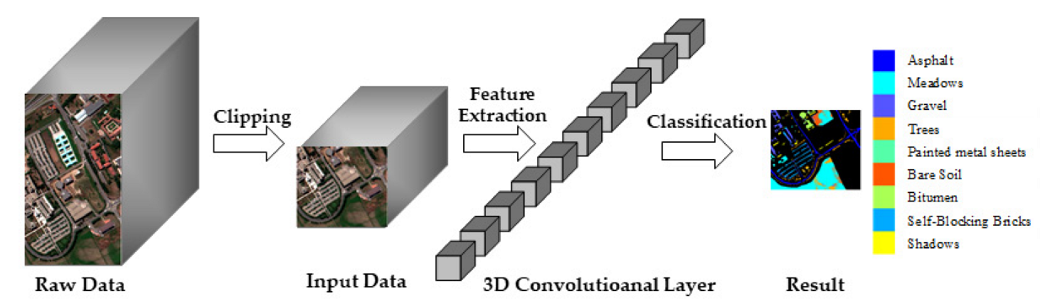
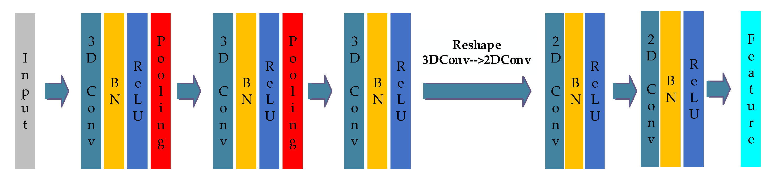
2.1. 3D–2D Hybrid Convolution

Two dimensional convolution for HSI classification [50], as shown in Figure 1, is generally divided into the following three steps: data dimension reduction (DR), feature extraction, and classification. DR is performed to reduce the spectral dimension of original HSI data. The main purpose is to reduce the number of HSI spectra, remove the redundancy between spectra, and facilitate subsequent feature extraction. Feature extraction uses a convolution operation to extract features from data. The 2D convolution operation for reduced HSI is similar to that for the ordinary image, except the difference in the number of channels. The number of channels in reduced HSI depends on the dimensionality reduction operation. The 2D feature information of the reduced HSI can be obtained after several runs of convolution operations. Classification refers to the classification function used, such as SoftMax, to analyze the feature extracted from the convolution layer and to obtain specific classes. The 2D convolution model is simple and the number of parameters is small, but the extracted features lack the spectral dimension, thereby reducing the classification performance for HSI.

3DCNN is used to extract the spatial–spectral joint features of HSI [51], as shown in Figure 2. Unlike 2D, 3D convolution can be directly applied on the raw HSI data, and can conduct convolution in both spatial and spectral dimensions. Compared to 2D convolution, the features obtained from 3D convolution contain additional spectral dimension and can be used to improve classification performance. However, the use of 3DCNN has the problems of increased model computation, a large number of parameters, and difficult training process.

There are certain shortcomings in using 2D or 3D convolution alone. To solve this problem, many researchers proposed the use of 3D–2D [52,53] hybrid convolution, as shown in Figure 3. Firstly, 3DCNN is used to extract the spatial–spectral joint features. Then, the last two dimensions of the features extracted by the 3D convolution layer are combined to achieve dimension reduction. The data after dimension reduction are used as the input of the 2D convolution layer to further extract more abstract spatial features. The use of hybrid convolution not only ensures the feature extraction ability, but also reduces the complexity and number of parameters of the model, which is easier for model training.

2.2. Dropout and Dropblock

Overfitting is a problem that is encountered in deep learning. When the number of training samples is low, the model learns the unique features from a few samples and ignores more general features, resulting in good performance in training and poor performance in testing. To solve this problem, researchers proposed some solutions, in which Dropout [54] was widely used in the application of deep learning due to its simple implementation and excellent results.

During forward propagation with Dropout, a neuron will stop working at a certain probability (Figure 4), which can make the model more generalizable, because the model does not heavily rely on specific local features. Dropout makes multiple neurons not necessarily appear in a dropout-based network every time. In this way, the updating of weights no longer depends on the joint action of hidden nodes with fixed relationships, which prevents some features from being effective under other specific features. Dropout forces the network to learn more robust features to achieve the purpose of enhancing the generalizability of the model. Dropout is generally used for the full connection layer in the deep learning model, rather than the convolution layer. This is because the convolution kernel corresponds to a region. If only a few neurons are stopped, the convolution kernel can learn information from the adjacent neurons, which does not improve the generalizability of the model. Dropblock [55] omits multiple neurons in continuous regions, as shown in Figure 5, the size of which are equal to that of the convolution kernel in the current layer. When the convolution kernel extracts a feature, it will lose the feature information of the relevant region. The network will focus on learning the features of other regions for classification, so as to improve the generalizability of the model.

The proposed model extracts the features of HSI using two convolution channels to improve the performance of HSI classification, and uses Dropblock in the convolution layer and Dropout in the full connection layer to manage the overfitting problem. The two feature extraction channels first use 3D convolution to extract features, and then carry out 2D convolution on the extracted features to further extract deeper features, which not only extracts discriminative features, but also enhances the generalizability of the model.

3. Proposed Model

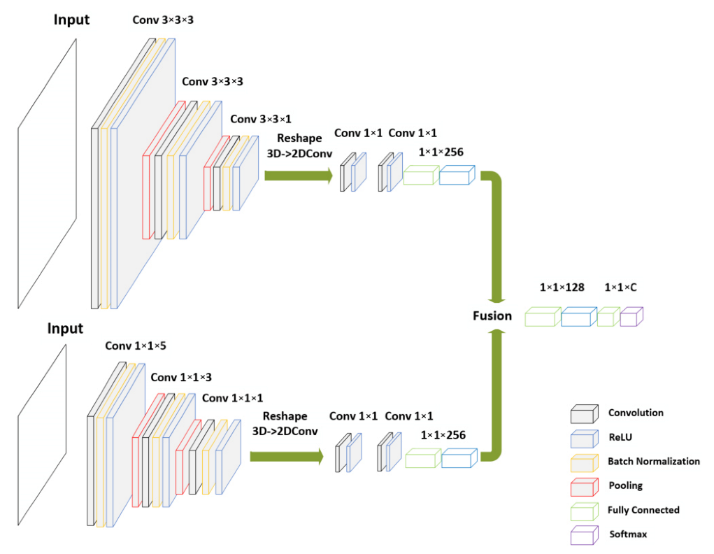
3.1. The Design of DSEN

As shown in Figure 6, the designed DSEN has two convolution channels. The upper channel is a spatial–spectral extraction channel, by which the spatial–spectral joint feature of HSI can be extracted from the data cube after dimension reduction. The lower channel is a spectral extraction channel focusing on the spectral feature representation of a specific pixel, by which the spectral features can be extracted from HSI. By adjusting the fusion proportion of the features extracted from the two feature extraction channels, the expression of spectral features can be enhanced in the fused features for better HSI classification. The model is mainly composed of the following four modules: data preprocessing, feature extraction, feature fusion, and classification. These modules are described in detail below.

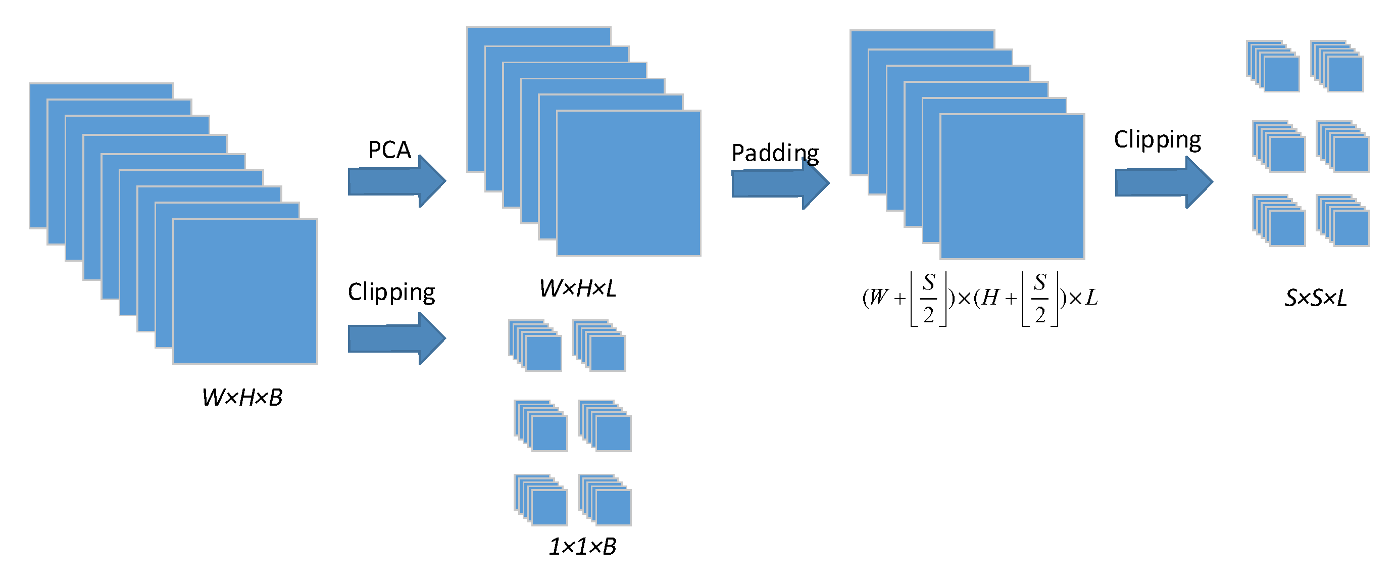
3.2. Data Preprocessing

The raw HSI cannot be directly used as the input of the proposed model, and needs to be processed first, as shown in Figure 7. It was assumed that the size of raw HSI data is $W\times H\times B$, where W and H are the length and width of the HSI, and B is the number of spectral bands.

For the spatial-spectral extraction channel, the size of input data is $S\times S\times L$, where L is much smaller than B, S is the length/width of the cube, L is the number of spectral segments. The classification refers to obtain the class of the central pixel of the data cube. In order to avoid the Hughes effect, PCA is used to reduce the dimension of the raw data. Assuming that L spectral bands are retained from the raw HSI, and hence the size of reduced HSI is $W\times H\times L$. In order to make full use of the data, mirror padding is firstly carried out on the four sides of the reduced HSI to obtain a data cube with size of $(W+\lfloor \frac{S}{2}\rfloor )\times (H+\lfloor \frac{S}{2}\rfloor )\times L$, and then the data are divided into cubes with size of $S\times S\times L$. Finally, the number of cubes is equal to the number of original pixels, and a total number of $W\times H$ data cubes are obtained.

For the spectral extraction channel, the input data size was $1\times 1\times B$. Because only spectral features were extracted from the spectral channel, the original data were standardized based on the spectral dimension, rather than global standardization. The purpose of this was to maximize the spectral dimension features. The standardized formula (Equation (1)) is:

$$x^{\prime }=\frac{x-\mu }{\delta }$$

(1)

where $x$ represents the original data, $\mu$ is the average, and $\delta$ is the standard deviation. The standardized data were divided into $W\times H$ blocks with a size of $1\times 1\times B$.

3.3. Feature Extraction

As shown in Figure 6, two extraction channels of the proposed model were implemented based on 3D–2D hybrid convolution, with similar structural settings as shown in Figure 8. Each extraction channel consists of five convolution modules, including three 3D convolution modules and two 2D convolution modules. Each 3D convolution module contains a convolution layer, Batch Normalization layer [56], RELU activation function layer, and 3D pooling layer. The Batch Normalization layer and RELU function effectively alleviate the problem of gradient disappearance, and accelerate the convergence speed of the model. The pooling layer retains the main features and reduces the calculation cost. The spatial–spectral extraction channel is similar to other CNN-based methods, using multiple convolutional layers to extract features [32]. In this paper, a 3D convolution kernel of size 3 × 3 instead of a larger size was used in the spatial–spectral extraction channel. Compared to a large convolution kernel, multiple small convolution kernels have a stronger feature extraction ability and lower computation cost.

It should be noted that in the design of the spectral channel, multiple 1 × 1 3D convolution kernels were adopted to extract the spectral features of HSI. The reason is that spectral features of neighbor pixels will be introduced when using large convolution kernels to extract HSI spectral features. When the number of samples is sufficient, the unrelated features brought by neighboring pixels is insignificant. However, if the number of samples is scarce, these will interfere with the expression of the spectral features of the specific pixel, thereby affecting classification performance. Using a convolution kernel with size 1 × 1 makes the model only focus on the specific pixel when extracting spectral features, which can solve the problem of introducing unrelated information and enhance the classification performance of the model.

As shown in Figure 8, there a reshape operation occurs after the last 3D convolution module. The purpose is to transform the output calculated by the 3D convolution module into the format that conforms to the subsequent 2D convolution module. The last two dimensions of the features extracted by 3D convolution are merged. The 2D convolution module contains a 2D convolution layer, batch normalization layer, and RELU function. The reason for removing the pooling layer is that the feature size is small after multiple downsampling operations. In the 2D convolution module, the size of the convolution kernel is 1 × 1, which can effectively integrate feature information. After the previous reshape operation, the number of channels is large, and the number of feature channels can be reduced by controlling the number of 2D convolution kernels.

3.4. Feature Fusion and Classification

The features extracted by the two extraction channels can be turned into a one-dimensional vector after flattening the layer. In order to obtain better classification results, the features extracted from the two extraction channels need to be fused. The method for this is to splice the two one-dimensional features into a new one-dimensional vector, and the dimension number of the new feature vector is the sum of the two feature dimensions.

Since the input data of the two extraction channels are different and the size of the convolution kernel is different, the feature dimensions obtained by the convolution layer are quite different, and the dimension of the feature extracted by the spatial–spectral channel is much larger than that of the spectral channel. If the features extracted from two extraction channels are directly fused, the feature expression of the spectral channel is weakened. In order to avoid this problem, this paper adopted the method described below. The features extracted by the two extraction channels are, respectively, passed through a fully connected layer first, and the output of the fully connected layer is then fused. Therefore, the dimension of the features extracted by the two channels can be determined by controlling the number of neurons in the fully connected layer. In this paper, this layer is referred to as the plastic layer. The features are further fused after passing through the plastic layer (Figure 9), and then are used to obtain the classification result by using the SoftMax function.

3.5. Parameter Setting

Table 1. Parameters of Spatial–Spectral channel, Spectral channel, and Fully connected layers.

Spatial–Spectral Channel			Spectral Channel			Fully Connected Layers
Layer	Channels/P	Size	Layer	Channels/P	Size	Layer	Type	Parameter
3DConv_1	16	1 × 1 × 5	3DConv_1	32	3 × 3 × 3	Dropout	Dropout	0.2
AvgPool_1	/	1 × 1 × 2	AvgPool_1	/	2 × 2 × 2	Dense_1	Fullyconnected + ReLU	128
DropBlock_1	0.15	1 × 1 × 3	DropBlock_1	0.25	3 × 3 × 3	Dropout	Dropout	0.2
3DConv_2	32	1 × 1 × 3	3DConv_2	32	3 × 3 × 5	Output	Fullyconnected + softmax	C
AvgPool_2	/	1 × 1 × 2	AvgPool_2	/	2 × 2 × 2
DropBlock_2	0.15	1 × 1 × 3	DropBlock_2	0.25	3 × 3 × 3
3DConv_3	64	1 × 1 × 1	3DConv_3	64	3 × 3 × 3
Dropout	0.2	/	Dropout	0.2	/
2DConv_1	256	1 × 1	2DConv_1	128	1 × 1
2DConv_2	128	1 × 1	2DConv_2	64	1 × 1
Flatten	/	/	Flatten	/	/
Dropout	0.2	/	Dropout	0.2	/
Plastic	/	256	Plastic	/	256

shows the basic parameters of the two feature extraction channels and the fully connected layers of the model, in which C represents the number of classes.

4. Experiments and Discussion

4.1. Experimental Data Sets

This paper used three public hyperspectral image datasets to test the classification performance of the proposed model, which are Indian Pines, University of Pavia and Salinas Scene, and are shown in

Table 2. Details of Indian Pines, University of Pavia, and Salinas Scene.

Indian Pines Dataset		University of Pavia Dataset		Salinas Scene Dataset
Land Cover Type	Samples	Land Cover Type	Samples	Land Cover Type	Samples
Alfalfa	46	Asphalt	6631	Brocoli_green_weeds_1	2009
Corn-notill	1428	Meadows	18,649	Brocoli_green_weeds_2	3726
Corn-min	830	Gravel	2099	Fallow	1976
Corn	237	Trees	3064	Fallow_rough_plow	1394
Grass/Pasture	483	Painted metal sheets	1345	Fallow_smooth	2678
Grass/Trees	730	Bare Soil	5029	Stubble	3959
Grass/Pasture-mowed	28	Bitumen	1330	Celery	3579
Hay-windrowed	478	Self-Blocking Bricks	3682	Grapes_untrained	11,271
Oats	20	Shadows	947	Soil_vinyard_develop	6203
Soybeans-notill	972			Corn_senesced_green_weeds	3278
Soybeans-min	2455			Lettuce_romaine_4wk	1068
Soybeans-clean	693			Lettuce_romaine_5wk	1927
Wheat	205			Lettuce_romaine_6wk	916
Woods	1265			Lettuce_romaine_7wk	1070
Bldg-Grass-Tree-Drives	386			Vinyard_untrained	7268
Stone-steel towers	93			Vinyard_vertical_trellis	1807
Total	10,349	Total	42,776	Total	54,129

in detail.

The Indian Pines (IP) dataset was collected using the AVIRIS sensor in the Indian Pines experimental field in northwest Indiana. The size of pixels is 145 × 145, and there are 224 spectral bands. The wavelength range is 400–2500 nm. This dataset mainly includes about two-thirds agriculture, one-third forest, and a small part natural vegetation. The data excluding crops with coverage less than 5% contain two roads, one railway, low-density houses and buildings, and are divided into 16 classes. The number of bands is reduced to 200 by removing 24 bands in water coverage area.

The University of Pavia (UP) dataset was obtained using an ROSIS sensor during flight over Pavia, northern Italy. The Pavia University scene is composed of 610 × 340 pixels with 103 spectral bands located in the wavelength range of 430–860 nm. The ground cover is divided into 9 urban land cover classes.

Salinas Scene (SA) dataset was captured by AVIRIS sensor at Salinas Valley, California. The data contains 512 × 217 pixels with a spatial resolution of 3.7 m and a total of 224 spectral bands. The data has 204 spectral bands after removing 20 water absorption bands. This dataset is divided into 16 classes, mainly composed of crops.

4.2. Experimental Setup

The training and testing of network models in this paper were carried out on the same server. The server hardware configuration was as follows: Intel (R) Xeon(R) Silver 4114 CPU @ 2.20GHz, 64GB RAM, and RTX2060 GPU with 6GB memory. Software configuration was as follows: Windows 10 [57], Python 3.7.0 [58], Tensorflow 2.3.0 [59], and Cuda 10.1 [60].

In order to verify the effectiveness of the proposed model, this paper used the overall accuracy (OA), average accuracy (AA) and Kappa coefficient to evaluate the HSI classification performance. OA is the ratio of the number of correctly classified samples to the total test sample. AA represents the mean classification accuracy of all classes. The Kappa co-efficient is used to test consistency and measure classification accuracy. DSEN was compared with HybridSN [32], MAPC [10], MFFN [44] and DC-CNN [39]. The dataset was randomly divided into 70% for training and 30% for testing first, and then the upper limit samples for each class were set to 5, 10 and 15, respectively, when selecting training samples. In other words, the number of training samples for each class was less than or equal to 5, 10 and 15 in the experiments. In the training process, the optimizer was Adam, the learning rate was 0.001, the decay rate was 0.000001, and the batch size was 16.

The plastic layer in the model controls the proportion of feature fusion of the two channels, and different fusion ratios have different effects on the classification performance. In order to clarify the influence, a series of experiments were conducted on different fusion ratios of the spatial–spectral channel (window size of input data: 25 × 25) and the spectral channel. The experimental results of model testing are presented in

Table 3. Classification performance of different fusion ratios (OA, Training sample = 10).

Dataset	4:1	3:1	2:1	1:1	1:2	1:3	1:4
IP	75.31	76.49	77.02	77.94	76.61	75.15	74.61
UP	85.19	86.66	87.51	88.53	86.18	85.35	84.02
SA	94.45	95.41	95.98	96.35	95.45	94.13	93.06

. The experimental result for the classification performance was optimum when the proportion was 1:1. When changing the fusion proportion of the two categories of features, the performance experienced different degrees of decline, so we selected 1:1 as the fusion rate, and this setting was used in all subsequent experiments.

In order to confirm the influence of the window size S of the input data for the spatial–spectral channel, experiments were carried out with different values of S. The number of training samples in the experiment was 10. The classification results of model testing are listed in

Table 4. Performance of different window sizes (OA).

Dataset	21 × 21	23 × 23	25 × 25	27 × 27
IP	71.80	75.23	77.75	77.89
UP	79.41	84.50	88.05	88.84
SA	92.18	94.06	96.31	96.01

. The time consumed with different S is shown in

Table 5. The total training and testing time of different window sizes (s).

Dataset	21 × 21	23 × 23	25 × 25	27 × 27
IP	87.03	93.04	99.12	120.68
UP	52.18	52.75	57.00	73.56
SA	74.47	79.41	85.70	98.31

. With the increase in S, the performance of the model improved. The performance improvement is obvious with S from 21 × 21 to 27 × 27, but it also increases the complexity of the model, the amount of calculation required, and the time consumed. When S = 27 × 27, compared to S = 25 × 25, the performance is slightly improved, but the time consumption is obviously increased. Therefore, in the subsequent experiments, the window size for the spatial–spectral channel is set to 25 × 25.

4.3. Experimental Results and Analysis

4.3.1. Experimental Result

Figure 10 shows the influence of a different number of training samples on classification accuracy for each dataset. Figure 11 shows the training process of DSEN in a different number of training samples. The model begins to converge when epoch = 50, which proves that DSEN has the ability of rapid convergence. When epoch = 100, the loss and accuracy of the model tend to remain stable without obvious fluctuations. With the increase in the number of training samples, the fluctuation of loss is lower, and the convergence is faster.

Due to the 3D–2D convolution used by DSEN, the number of parameters also reduced.

Table 6. Total Model Training and Testing Time (s).

Model	Indian Pines	University of Pavia	Salinas Scene
HybridSN	90.20	34.18	54.43
MAPC	706.67	1541.16	1469.79
MFFN	171.88	102.36	136.21
DC-CNN	32.33	30.44	30.46
DSEN	98.10	58.12	87.32

shows the total training (10 training samples) and testing time per model. Compared with MAPC, the time consumption of the model based on CNN significantly reduced. The time consumption of DC-CNN was lowest because it only uses 2D convolution and 1D convolution. Compared with HybridSN, DSEN has fewer parameters, but increased time consumption. This is because DSEN has more network layers and a more complex model structure.

Although MFFN also uses 3D convolution to extract features, there is no approach to reduce overfitting. The model performs well when the number of samples is sufficient, but will aggravate the overfitting phenomenon when few samples are available. Therefore, the final performance of MFFN is weakened.

DC-CNN is also a dual-channel design, which is divided into two channels of 2D convolution and 1D convolution. Its performance is stronger than HybridSN and MFFN, which also proves that, when the sample number is lower, enhancing the expression of spectral features can improve the classification performance.

4.3.2. Comparison and Analysis

To investigate the role of spatial–spectral and spectral channels in DSEN, this paper conducted experiments relying on a single channel. In the experiment, only one channel was used to extract features for classification. The experimental results were compared with that of Dual-channel, as shown in

Table 7. Experimental results using spatial–spectral channel, spectrum channel, and dual-channel under 5, 10, and 15 training samples per class from IP, UP, and SA, respectively (OA).

Sample	Spatial-Spectral			Spectral			Dual-Channel
	IP	UP	SA	IP	UP	SA	IP	UP	SA
5	61.59	75.77	91.87	45.21	61.27	72.31	69.47	80.54	93.24
10	71.01	83.80	94.17	50.19	68.35	75.51	77.94	88.53	96.35
15	78.55	87.69	95.71	54.03	72.91	84.51	83.94	90.64	97.61

.

Spatial–spectral joint features are extracted using the spatial–spectral channel. The joint features are very effective for HSI classification. So, the performance gap between the spatial–spectral channel and dual-channel is significantly smaller than that between the spectral channel and dual-channel.

Although the classification performance of the feature extracted by the spectral channel is not satisfactory when the number of HSI samples is low, spectral features can be combined with other features to enhance the expression of spectral features, which can significantly improve the classification performance of the model. It also proves that fully exploiting the spectral information of pixels is effective in HSI classification under scarce samples.

Table 8. Classification results of models.

Training Sample	Model	Indian Pines			University of Pavia			Salinas Scene
		OA (%)	AA (%)	Kappa	OA (%)	AA (%)	Kappa	OA (%)	AA (%)	Kappa
5	HybridSN	57.25	72.54	0.53	71.38	72.24	0.67	86.93	89.06	0.86
	MAPC	67.27	78.32	0.63	76.20	79.33	0.69	92.57	94.84	0.89
	MFFN	44.44	57.75	0.39	56.94	59.97	0.51	59.25	59.43	0.56
	DC-CNN	60.33	72.77	0.54	73.52	74.76	67.59	89.70	90.72	0.88
	DSEN	69.47	81.11	0.66	80.54	83.63	0.78	93.24	94.09	0.93
10	HybridSN	65.50	76.49	0.61	77.72	79.86	0.75	94.18	94.87	0.94
	MAPC	76.14	80.59	0.75	83.58	86.65	0.81	96.04	97.01	0.96
	MFFN	58.24	73.06	0.54	58.22	64.34	0.53	80.15	82.80	0.79
	DC-CNN	77.88	85.61	0.75	82.14	85.20	0.80	95.42	93.51	0.92
	DSEN	77.94	86.82	0.75	88.53	90.00	0.87	96.35	97.10	0.96
15	HybridSN	66.06	79.24	0.62	86.88	89.05	0.85	95.31	95.98	0.95
	MAPC	82.71	90.06	0.80	89.78	92.35	0.89	97.24	97.09	0.96
	MFFN	68.32	79.67	0.65	70.08	75.89	0.66	88.87	90.32	0.88
	DC-CNN	79.94	90.12	0.78	87.57	89.58	0.86	96.28	96.95	0.96
	DSEN	83.94	91.55	0.82	90.64	91.45	0.89	97.61	97.96	0.97

provides the classification performance of model testing. Among the methods, MAPC is based on random forest and the rest are based on CNN. Among the CNN-based methods, DSEN demonstrated the best integrated classification performance and MFFN had the worst performance. The multi-channel based DSEN and DC-CNN performed better than the single-channel based HybridSN and MFFN, which indicates that the multi-channel design can improve the classification performance of the model. Compared with HybridSN and MFFN, MAPC and DSEN have a significant lead regardless of the number of training samples. Compared with MAPC, DSEN leads in terms of performance when the samples are extremely small, such as when sample = 5 or 10. When the number of samples increases to 15 for each class, the performance gap between the two methods is very small, but DSEN still has a marginal advantage.

Figure 12, Figure 13 and Figure 14 show the classification results of DSEN trained by different sample numbers on three datasets, respectively. The overall classification accuracy improves significantly as the number of training samples increases, and the correct rate for the individual class also improves. In some of the datasets, there is a large number of classification errors for one category with a training sample size of 5. This situation improves significantly as the training sample size increases. It is worth noting that most of the incorrectly classified pixel points are at the border of the classes, which is because the spatial neighborhood information of the pixel points is used in the classification, thereby the feature information of other classes is mixed in the feature extraction of the specific pixels, and affects the correct classification rate of the pixels by the model.

Figure 15, Figure 16 and Figure 17 show the classification results of each model on three datasets with training sample = 10, respectively. From the results, it can be seen that DSEN is superior to other methods in terms of overall classification accuracy, but it is worth noting that the accuracy of each method varies significantly between different classes. For example, on the UP dataset, DSEN is weaker than HybridSN and DC-CNN for the classification of Bare Soil, but the overall accuracy is better. The experimental results show that although the proposed method is relatively weak in a few cases, the overall classification performance is superior to the compared methods in almost all cases.

5. Conclusions

This paper designed a novel dual-channel network model including two convolutional channels, in which one channel utilized 3D–2D hybrid convolution to extract the joint spatial–spectral features and the other channel used 1 × 1 3D and 2D convolution to extract the spectral features. The performance of the model for HSI classification with few samples improved after enhancing the expression of spectral features based on feature fusion. Through the experiments performed on three public datasets, the results revealed that DSEN has significant advantages in HSI classification performance compared with several other deep learning methods, thereby proving the effectiveness of our method.

References

1. Shippert, P. Why Use Hyperspectral Imagery? Photogramm. Eng. Remote Sens. 2004, 70, 377–396. [Google Scholar]
2. Yadav, B.K.; Lucieer, A.; Baker, S.C.; Jordan, G.J. Tree crown segmentation and species classification in a wet eucalypt forest from airborne hyperspectral and LiDAR data. Int. J. Remote Sens. 2021, 42, 7952–7977. [Google Scholar] [CrossRef]
3. Pacheco, A.; Bannari, A.; Deguise, J.C.; McNairn, H.; Staenz, K. Application of hyperspectral remote sensing for LAI estimation in precision farming. In Proceedings of the 23rd Canadian Remote Sensing Symposium, Sainte-Foy, QC, Canada, 21–24 August 2001; pp. 281–287. [Google Scholar]
4. Gevaert, C.M.; Suomalainen, J.; Tang, J.; Kooistra, L. Generation of spectral–temporal response surfaces by combining multispectral satellite and hyperspectral UAV imagery for precision agriculture applications. IEEE J. Sel. Top. Appl. Earth Obs. Remote Sens. 2015, 8, 3140–3146. [Google Scholar] [CrossRef]
5. Dale, L.M.; Thewis, A.; Boudry, C.; Rotar, I.; Dardenne, P.; Baeten, V.; Pierna, J.A.F. Hyperspectral imaging applications in agriculture and agro-food product quality and safety control: A review. Appl. Spectrosc. Rev. 2013, 48, 142–159. [Google Scholar] [CrossRef]
6. Gao, Y.; Li, W.; Zhang, M.; Wang, J.; Sun, W.; Tao, R.; Du, Q. Hyperspectral and multispectral classification for coastal wetland using depthwise feature interaction network. IEEE Trans. Geosci. Remote Sens. 2021, 60, 1–15. [Google Scholar] [CrossRef]
7. Manolakis, D.; Shaw, G. Detection algorithms for hyperspectral imaging applications. IEEE Signal Process. Mag. 2002, 19, 29–43. [Google Scholar] [CrossRef]
8. Sun, S.; Zhong, P.; Xiao, H.; Liu, F.; Wang, R. An active learning method based on Markov random fields for hyperspectral images classification. In Proceedings of the 2015 7th Workshop on Hyperspectral Image and Signal Processing: Evolution in Remote Sensing (WHISPERS), Tokyo, Japan, 2–5 June 2015. [Google Scholar]
9. Ren, Y.; Zhang, Y.; Li, L. A spectral-spatial hyperspectral data classification approach using random forest with label constraints. In Proceedings of the 2014 IEEE Workshop on Electronics, Computer and Applications, Ottawa, ON, Canada, 8–9 May 2014. [Google Scholar]
10. Liu, B.; Guo, W.; Chen, X.; Gao, K.; Zuo, X.; Wang, R.; Yu, A. Morphological attribute profile cube and deep random forest for small sample classification of hyperspectral image. IEEE Access 2020, 8, 117096–117108. [Google Scholar] [CrossRef]
11. Agarwal, A.; El-Ghazawi, T.; El-Askary, H.; Le-Moigne, J. Efficient hierarchical-PCA dimension reduction for hyperspectral imagery. In Proceedings of the 2007 IEEE International Symposium on Signal Processing and Information Technology, Giza, Egypt, 15–18 December 2007. [Google Scholar]
12. Vaddi, R.; Prabukumar, M. Probabilistic PCA based hyper spectral image classification for remote sensing applications. In International Conference on Intelligent Systems Design and Applications; Springer: Cham, Switzerland, 2018. [Google Scholar]
13. Wang, J.; Chang, C.-I. Independent component analysis-based dimensionality reduction with applications in hyperspectral image analysis. IEEE Trans. Geosci. Remote Sens. 2006, 44, 1586–1600. [Google Scholar] [CrossRef]
14. Zhang, Z.; Geiger, J.; Pohjalainen, J.; Mousa, A.E.D.; Jin, W.; Schuller, B. Deep learning for environmentally robust speech recognition: An overview of recent developments. ACM Trans. Intell. Syst. Technol. (TIST) 2018, 9, 1–28. [Google Scholar] [CrossRef]
15. Young, T.; Hazarika, D.; Poria, S.; Cambria, E. Recent trends in deep learning based natural language processing. IEEE Comput. Intell. Mag. 2018, 13, 55–75. [Google Scholar] [CrossRef]
16. Voulodimos, A.; Doulamis, N.; Doulamis, A.; Protopapadakis, E. Deep learning for computer vision: A brief review. Comput. Intell. Neurosci. 2018, 2018, 7068349. [Google Scholar] [CrossRef] [PubMed]
17. Li, S.; Song, W.; Fang, L.; Chen, Y.; Ghamisi, P.; Benediktsson, J.A. Deep learning for hyperspectral image classification: An overview. IEEE Trans. Geosci. Remote Sens. 2019, 57, 6690–6709. [Google Scholar] [CrossRef]
18. Hinton, G.E.; Ruslan, R.S. Reducing the dimensionality of data with neural networks. Science 2006, 313, 504–507. [Google Scholar] [CrossRef]
19. Chen, Y.; Lin, Z.; Zhao, X.; Wang, G.; Gu, Y. Deep learning-based classification of hyperspectral data. IEEE J. Sel. Top. Appl. Earth Obs. Remote Sens. 2014, 7, 2094–2107. [Google Scholar] [CrossRef]
20. Ma, X.; Wang, H.; Geng, J. Spectral–spatial classification of hyperspectral image based on deep auto-encoder. IEEE J. Sel. Top. Appl. Earth Obs. Remote Sens. 2016, 9, 4073–4085. [Google Scholar] [CrossRef]
21. Chen, Y.; Zhao, X.; Jia, X. Spectral–spatial classification of hyperspectral data based on deep belief network. IEEE J. Sel. Top. Appl. Earth Obs. Remote Sens. 2015, 8, 2381–2392. [Google Scholar] [CrossRef]
22. Fukushima, K. A self-organizing neural network model for a mechanism of pattern recognition unaffected by shift in position. Biol. Cybern. 1980, 36, 193–202. [Google Scholar] [CrossRef] [PubMed]
23. Chen, Y.; Jiang, H.; Li, C.; Jia, X.; Ghamisi, P. Deep feature extraction and classification of hyperspectral images based on convolutional neural networks. IEEE Trans. Geosci. Remote Sens. 2016, 54, 6232–6251. [Google Scholar] [CrossRef]
24. Zhang, M.; Wei, L.; Qian, D. Diverse region-based CNN for hyperspectral image classification. IEEE Trans. Image Process. 2018, 27, 2623–2634. [Google Scholar] [CrossRef]
25. Zhang, L.; Zhang, L.; Bo, D. Deep learning for remote sensing data: A technical tutorial on the state of the art. IEEE Geosci. Remote Sens. Mag. 2016, 4, 22–40. [Google Scholar] [CrossRef]
26. Chang, Y.; Yan, L.; Fang, H.; Zhong, S.; Liao, W. HSI-DeNet: Hyperspectral image restoration via convolutional neural network. IEEE Trans. Geosci. Remote Sens. 2018, 57, 667–682. [Google Scholar] [CrossRef]
27. Yu, C.; Zhao, M.; Song, M.; Wang, Y.; Li, F.; Han, R.; Chang, C.I. Hyperspectral image classification method based on CNN architecture embedding with hashing semantic feature. IEEE J. Sel. Top. Appl. Earth Obs. Remote Sens. 2019, 12, 1866–1881. [Google Scholar] [CrossRef]
28. He, N.; Paoletti, M.E.; Haut, J.M.; Fang, L.; Li, S.; Plaza, A.; Plaza, J. Feature extraction with multiscale covariance maps for hyperspectral image classification. IEEE Trans. Geosci. Remote Sens. 2018, 57, 755–769. [Google Scholar] [CrossRef]
29. Paoletti, M.E.; Haut, J.M.; Plaza, J.; Plaza, A. A new deep convolutional neural network for fast hyperspectral image classification. ISPRS J. Photogramm. Remote Sens. 2018, 145, 120–147. [Google Scholar] [CrossRef]
30. Sellami, A.; Farah, M.; Farah, I.R.; Solaiman, B. Hyperspectral imagery classification based on semi-supervised 3-D deep neural network and adaptive band selection. Expert Syst. Appl. 2019, 129, 246–259. [Google Scholar] [CrossRef]
31. Liu, H.; Li, W.; Xia, X.G.; Zhang, M.; Gao, C.Z.; Tao, R. Central Attention Network for Hyperspectral Imagery Classification. IEEE Trans. Neural Netw. Learn. Syst. 2022. [Google Scholar] [CrossRef]
32. Roy, S.K.; Krishna, G.; Dubey, S.R.; Chaudhuri, B.B. HybridSN: Exploring 3-D–2-D CNN feature hierarchy for hyperspectral image classification. IEEE Geosci. Remote Sens. Lett. 2019, 17, 277–281. [Google Scholar] [CrossRef]
33. Li, Y.; Xie, W.; Li, H. Hyperspectral image reconstruction by deep convolutional neural network for classification. Pattern Recognit. 2017, 63, 371–383. [Google Scholar] [CrossRef]
34. Zhang, T.; Fu, Y.; Wang, L.; Huang, H. Hyperspectral image reconstruction using deep external and internal learning. In Proceedings of the IEEE/CVF International Conference on Computer Vision, Seoul, Korea, 27 October–2 November 2019. [Google Scholar]
35. Wang, G.; Ye, J.C.; De Man, B. Deep learning for tomographic image reconstruction. Nat. Mach. Intell. 2020, 2, 737–748. [Google Scholar] [CrossRef]
36. Zhang, Y.; Li, W.; Zhang, M.; Qu, Y.; Tao, R.; Qi, H. Topological structure and semantic information transfer network for cross-scene hyperspectral image classification. IEEE Trans. Neural Netw. Learn. Syst. 2021. [Google Scholar] [CrossRef]
37. Li, X.; Ding, M.; Aleksandra, P. Deep feature fusion via two-stream convolutional neural network for hyperspectral image classification. IEEE Trans. Geosci. Remote Sens. 2019, 58, 2615–2629. [Google Scholar] [CrossRef]
38. Kong, Y.; Wang, X.; Cheng, Y. Spectral–spatial feature extraction for HSI classification based on supervised hypergraph and sample expanded CNN. IEEE J. Sel. Top. Appl. Earth Obs. Remote Sens. 2018, 11, 4128–4140. [Google Scholar] [CrossRef]
39. Zhang, H.; Li, Y.; Zhang, Y.; Shen, Q. Spectral-spatial classification of hyperspectral imagery using a dual-channel convolutional neural network. Remote Sens. Lett. 2017, 8, 438–447. [Google Scholar] [CrossRef]
40. Li, W.; Gao, Y.; Zhang, M.; Tao, R.; Du, Q. Asymmetric Feature Fusion Network for Hyperspectral and SAR Image Classification. IEEE Trans. Neural Netw. Learn. Syst. 2022. [Google Scholar] [CrossRef] [PubMed]
41. Zhang, M.; Li, W.; Du, Q.; Gao, L.; Zhang, B. Feature extraction for classification of hyperspectral and LiDAR data using patch-to-patch CNN. IEEE Trans. Cybern. 2018, 50, 100–111. [Google Scholar] [CrossRef]
42. Zhang, M.; Li, W.; Tao, R.; Li, H.; Du, Q. Information fusion for classification of hyperspectral and LiDAR data using IP-CNN. IEEE Trans. Geosci. Remote Sens. 2021, 60, 1–12. [Google Scholar] [CrossRef]
43. Yang, J.; Wu, C.; Du, B.; Zhang, L. Enhanced Multiscale Feature Fusion Network for HSI Classification. IEEE Trans. Geosci. Remote Sens. 2021, 59, 10328–10347. [Google Scholar] [CrossRef]
44. Ge, Z.; Cao, G.; Li, X.; Fu, P. Hyperspectral image classification method based on 2D–3D CNN and multibranch feature fusion. IEEE J. Sel. Top. Appl. Earth Obs. Remote Sens. 2020, 13, 5776–5788. [Google Scholar] [CrossRef]
45. Sellami, A.; Abbes, A.B.; Barra, V.; Farah, I.R. Fused 3-D spectral-spatial deep neural networks and spectral clustering for hyperspectral image classification. Pattern Recognit. Lett. 2020, 138, 594–600. [Google Scholar] [CrossRef]
46. Li, Z.; Wang, T.; Li, W.; Du, Q.; Wang, C.; Liu, C.; Shi, X. Deep multilayer fusion dense network for hyperspectral image classification. IEEE J. Sel. Top. Appl. Earth Obs. Remote Sens. 2020, 13, 1258–1270. [Google Scholar] [CrossRef]
47. Gao, K.; Liu, B.; Yu, X.; Qin, J.; Zhang, P.; Tan, X. Deep relation network for hyperspectral image few-shot classification. Remote Sens. 2020, 12, 923. [Google Scholar] [CrossRef]
48. He, X.; Chen, Y.; Pedram, G. Heterogeneous transfer learning for hyperspectral image classification based on convolutional neural network. IEEE Trans. Geosci. Remote Sens. 2019, 58, 3246–3263. [Google Scholar] [CrossRef]
49. Zhang, Y.; Li, W.; Tao, R.; Peng, J.; Du, Q.; Cai, Z. Cross-scene hyperspectral image classification with discriminative cooperative alignment. IEEE Trans. Geosci. Remote Sens. 2021, 59, 9646–9660. [Google Scholar] [CrossRef]
50. Hu, W.-S.; Li, H.C.; Pan, L.; Li, W.; Tao, R.; Du, Q. Spatial–spectral feature extraction via deep ConvLSTM neural networks for hyperspectral image classification. IEEE Trans. Geosci. Remote Sens. 2020, 58, 4237–4250. [Google Scholar] [CrossRef]
51. Liu, B.; Yu, X.; Zhang, P.; Tan, X.; Wang, R.; Zhi, L. Spectral–spatial classification of hyperspectral image using three-dimensional convolution network. J. Appl. Remote Sens. 2018, 12, 016005. [Google Scholar]
52. Mohan, A.; Venkatesan, M. HybridCNN based hyperspectral image classification using multiscale spatiospectral features. Infrared Phys. Technol. 2020, 108, 103326. [Google Scholar] [CrossRef]
53. Paul, A.; Sanghamita, B.; Nabendu, C. SSNET: An improved deep hybrid network for hyperspectral image classification. Neural Comput. Appl. 2021, 33, 1575–1585. [Google Scholar] [CrossRef]
54. Srivastava, N.; Hinton, G.; Krizhevsky, A.; Sutskever, I.; Salakhutdinov, R. Dropout: A simple way to prevent neural networks from overfitting. J. Mach. Learn. Res. 2014, 15, 1929–1958. [Google Scholar]
55. Golnaz, G.; Lin, T.-Y.; Le, Q.V. Dropblock: A regularization method for convolutional networks. arXiv 2018, arXiv:1810.12890. [Google Scholar]
56. Sergey, I.; Szegedy, C. Batch normalization: Accelerating deep network training by reducing internal covariate shift. In International Conference on Machine Learning; PMLR: New York, NY, USA, 2015. [Google Scholar]
57. Available online: https://www.microsoft.com/zh-cn/windows?r=1 (accessed on 2 August 2022).
58. Available online: https://www.python.org/ (accessed on 2 August 2022).
59. Available online: https://www.tensorflow.org/?hl=zh-cn (accessed on 2 August 2022).
60. Available online: https://developer.nvidia.com/cuda-toolkit (accessed on 2 August 2022).
Figure 1. HSI Classification Based on 2DCNN.
Electronics 11 02540 g001
Figure 2. HSI Classification Process Based on 3DCNN.
Electronics 11 02540 g002
Figure 3. HSI Classification Based on 3D–2DCNN.
Electronics 11 02540 g003
Figure 4. The difference between a standard neural network model and a neural network using Dropout (The red solid circle represents the dropped-out neurons).
Electronics 11 02540 g004
Figure 5. The difference between Dropout and Dropblock (Dropout omits multiple neurons randomly and Dropblock omits multiple neurons in continuous regions).
Electronics 11 02540 g005
Figure 6. DSEN (The upper channel is a spatial–spectral extraction channel and the lower channel is a spectral extraction channel).
Electronics 11 02540 g006
Figure 7. Data preprocessing.
Electronics 11 02540 g007
Figure 8. Feature extraction.
Electronics 11 02540 g008
Figure 9. Feature fusion process based on concat.
Electronics 11 02540 g009
Figure 10. Classification accuracy for different datasets when the number of training samples is increased. (a) IP; (b) UP; (c) SA.
Electronics 11 02540 g010
Figure 11. Training process for different number of training samples, (a) Training process for sample = 5; (b) Training process for sample = 10; (c) Training process for sample = 15.
Electronics 11 02540 g011
Figure 12. Classification maps on the IP dataset based on different number of training samples. (a) Sample = 5; (b) Sample = 10; (c) Sample = 15.
Electronics 11 02540 g012
Figure 13. Classification maps on the UP dataset based on different number of training samples. (a) Sample = 5; (b) Sample = 10; (c) Sample = 15.
Electronics 11 02540 g013
Figure 14. Classification maps on the SA dataset based on different number of training samples. (a) Sample = 5; (b) Sample = 10; (c) Sample = 15.
Electronics 11 02540 g014
Figure 15. Classification maps of different model (training sample = 10) on the IP dataset. (a) Ground-truth map. (b) HybridSN. (c) MAPC. (d) MFFN. (e) DC-CNN. (f) DSEN.
Electronics 11 02540 g015
Figure 16. Classification maps of different model (training sample = 10) on the UP dataset. (a) Ground-truth map. (b) HybridSN. (c) MAPC. (d) MFFN. (e) DC-CNN. (f) DSEN.
Electronics 11 02540 g016
Figure 17. Classification maps of different model (training sample = 10) on the SA dataset. (a) Ground-truth map. (b) HybridSN. (c) MAPC. (d) MFFN. (e) DC-CNN. (f) DSEN.
Electronics 11 02540 g017