A Reconfigurable Modular Vehicle Control Strategy Based on an Improved Artificial Potential Field

Abstract

The reconfigurable modular vehicle group can transform into different configurations according to different requirements to be competent for various tasks and scenarios and to facilitate the utilization of robots in unstructured scenarios. Efficient and effective reconfiguration strategies and path planning are essential for improving the performance of modular vehicle groups. First, a multi-sensing four-wheel-drive Mecanum vehicle was built, which was equipped with UWB positioning (based on wireless carrier communication technology), communication based on ESP8266 modules, ultrasonic ranging and a magnetic structure. Second, concerning the indoor storage environment, a UWB two-way bilateral ranging and positioning system was designed, and the experimental accuracy for positioning could reach ±0.1 m. Third, a path planning strategy based on the improved artificial potential field method was adopted. According to the target configuration as well as the obstacle avoidance requirements, the motion space was converted into a gravitational field and a repulsive force field, and the vector superposition of the gradients was used for the path planning of each vehicle in turn. Depending on the reconfiguration command and the connection matrix, the magnetic structure would strengthen or disconnect the vehicle group configuration. Finally, the vehicle reconfiguration from the stochastic dispersion state to the target configuration and the transition between different configurations were accomplished using the proposed strategy in both simulations and experiments.

1. Introduction

At present, most factories still use manual transportation, which features low automation. From the perspective of the entire production cycle, more than 90% of the time is used for loading and unloading, transshipment, etc., and inefficient manual transportation significantly limits production efficiency. An Automated Guided Vehicle (AGV) is automated transportation equipment that integrates machinery, electricity, control and sensing, which has been widely used in automobiles, manufacturing, logistics, storage and other fields. Compared with manual transportation, an AGV has the advantages of a lower cost, higher efficiency, higher accuracy and easier management [1].

For complicated unstructured spaces, a smaller and more flexible reconfigurable modular vehicle group can effectively increase the utilization of the whole system and further improve the overall automation level. Compared with traditional AGVs, the reconfigurable modular vehicle group can change the configuration of the group according to the requirements of special tasks and scenarios, which increases the diversity of configuration and adaptability to unknown environments.

With the goal of moving freely in a small space, many companies have designed a variety of omnidirectional mobile vehicles. This kind of vehicle usually has three degrees of freedom and can move freely in all directions, including moving forward and backward, rotating, multi-angle lateral movement, etc. [2].

Path planning is finding the shortest possible path between two points [3]. There exist many mature algorithms for path planning, such as Breadth First Search (BFS) and Depth First Search (DFS), and further optimization algorithms include the Dijkstra algorithm [4], A* algorithm [5], Bellman–Ford algorithm [6], etc., which traverse the map structure based on the path weight and iteratively calculate the path cost during the search, followed by backtracking to obtain an optimal solution when the calculation is completed. The artificial potential field method abstracts the motion of a robot in the surrounding environment into motion in an artificial gravitational field [7]. The target point generates “gravity” to the mobile robot, and the obstacle generates “repulsion” to the mobile robot. Finally, the motion of the mobile robot is controlled by calculating the resultant force [8]. The path planned by the potential field method is generally smooth and safe, but the results obtained may fall into local optimal solutions [9,10].

Multiple AGVs need to consider the possibility of route conflicts, node occupancy, etc., in path optimization. Nishi et al. [11] established a colored time Petri net to decompose the AGV scheduling model, which solved the conflict and deadlock problems (due to unreasonable scheduling and multiple AGVs coming into the blocking status to avoid collision) of the multi-AGV system. However, this method is computationally complex, and the efficiency is generally low when there is a large number of AGVs. Van et al. [12] proposed a distributed planning algorithm based on traffic rules, which reduces computational complexity. Konar et al. [13] used reinforcement learning to predict possible conflicts, and waiting times are planned in advance. However, this method requires a large amount of calculation, and the real-time performance of AGV planning is poor.

The reconfiguration rule of the reconfigurable modular vehicle group refers to the vehicle group moving to the corresponding position in the target configuration from a random dispersion state, and connecting as a whole in the original and final state. The reconfiguration strategy is very important for the reconfigurable modular vehicle group to complete various tasks. On the other hand, the path planning of the reconfigurable modular vehicle group focuses more on the reorganization process of multiple vehicles. Under the constraint of not colliding with obstacles and other vehicles, a unique path is determined for each vehicle in the group to accomplish the overall reconfiguration task.

The previous literature on the path planning of multiple vehicles mainly focuses on either search graph algorithms, such as the A* algorithm, or intelligent optimization algorithms, such as the ant colony algorithm and the particle swarm optimization algorithm. This paper designs and develops a group of multi-sensor reconfigurable vehicles from a systematic level, and bilateral UWB ranging and triangulation are utilized to construct a vehicle positioning system suitable for an indoor warehouse environment, due to its high positioning accuracy and strong anti-interference ability. According to the improved artificial potential field method, by taking any selectable position within the positioning range as the end point, the motion path of each vehicle is planned. Through simulations and experiments, the effectiveness of the proposed reconfiguration control strategy is demonstrated and verified.

The main contributions of this paper are summarized as follows: (i) A set of modular vehicle groups with electromagnets and ultrasonic obstacle avoidance abilities is designed and implemented; (ii) A Mecanum wheel is utilized in each vehicle, which guarantees high mobility; (iii) Based on the artificial potential field method for local path planning, the system has higher robustness, adaptability and functional versatility.

2. Reconfigurable Modular Vehicle

In order to improve control accuracy, the reconfigurable modular vehicle is required to be capable of free movement, connection and separation, the detection and avoidance of obstacles, communication and positioning and other functions through reasonable and efficient structural design. Each vehicle is equipped with four-motor-drive Mecanum wheels. The electric-driven magnetic structure can connect and separate modular vehicles. The ultrasonic module can detect obstacles in the environment. WiFi and UWB modules help to transmit a variety of vehicle information.

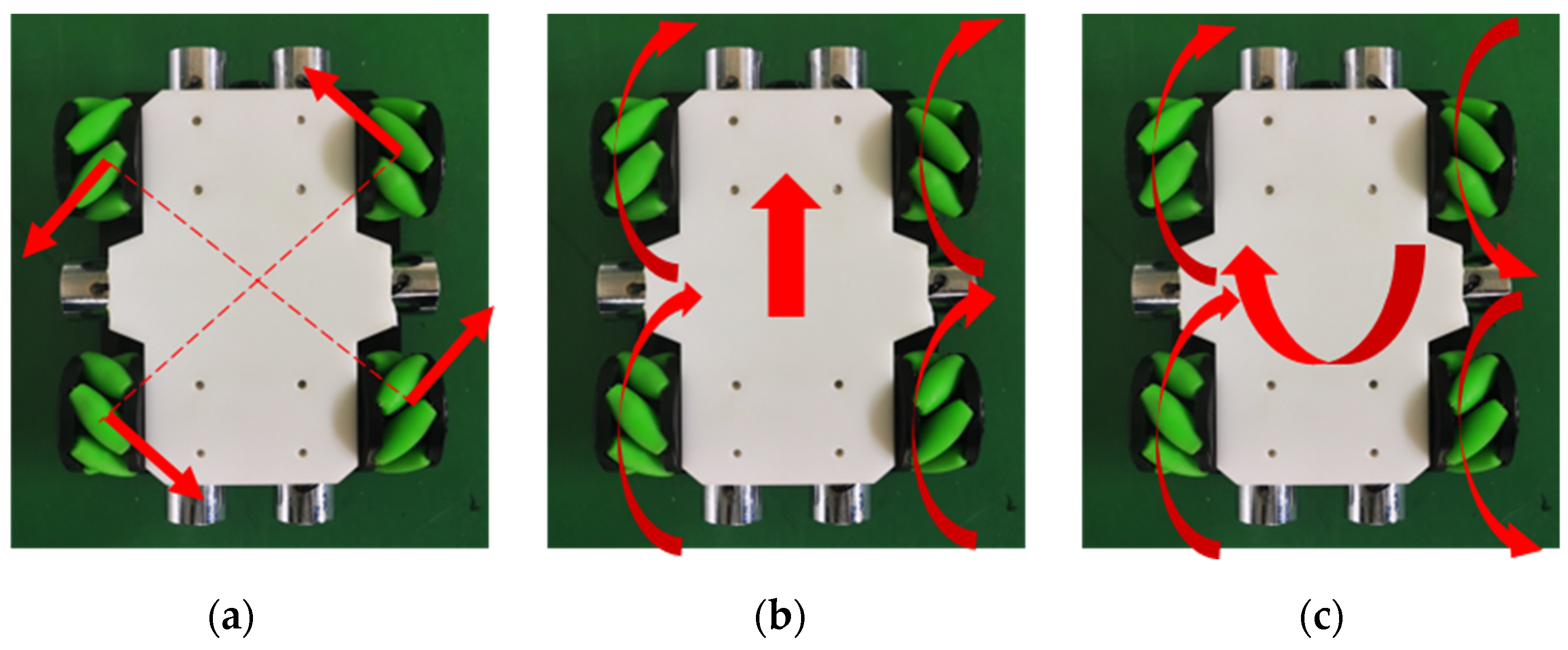
The structure and layout of the Mecanum wheel on the vehicle is shown in Figure 1. Using the forward kinematics and inverse kinematics equations of the Mecanum wheel, the motor speed is transformed into a motion vector; therefore, the modular vehicle can move omnidirectionally in the plane.

In order to reduce the influence of unpredictable random interference on the vehicle during the reconfiguration process, and to improve the robustness of the control strategy, the electric-driven magnetic structure is installed on both the x-axis surface and the y-axis surface of the modular vehicle, as shown in Figure 2a. The orders of the four magnetic structures on each vehicle are shown in Figure 2b. When the position of each vehicle meets the target configuration, the electromagnets in the corresponding direction are energized to enhance the connection stability of the configuration. When the vehicle group is determined to separate, the control system on the module vehicle disables the electromagnet in the corresponding direction.

During the process of reconfiguration, there may be obstacles in the motion path of each vehicle. Therefore, the modular vehicle is required to have the ability to identify and avoid obstacles. In this paper, ultrasonic obstacle detection modules are installed on the four plane directions of each modular vehicle, as shown in Figure 3. (Lidar is also an effective method to detect obstacles, which is not utilized here mainly because of its size and energy consumption). During the reconfiguration process, the ultrasonic probe is used to detect whether there are obstacles in the space, and at the same time, it is also used to judge its distance to other vehicles.

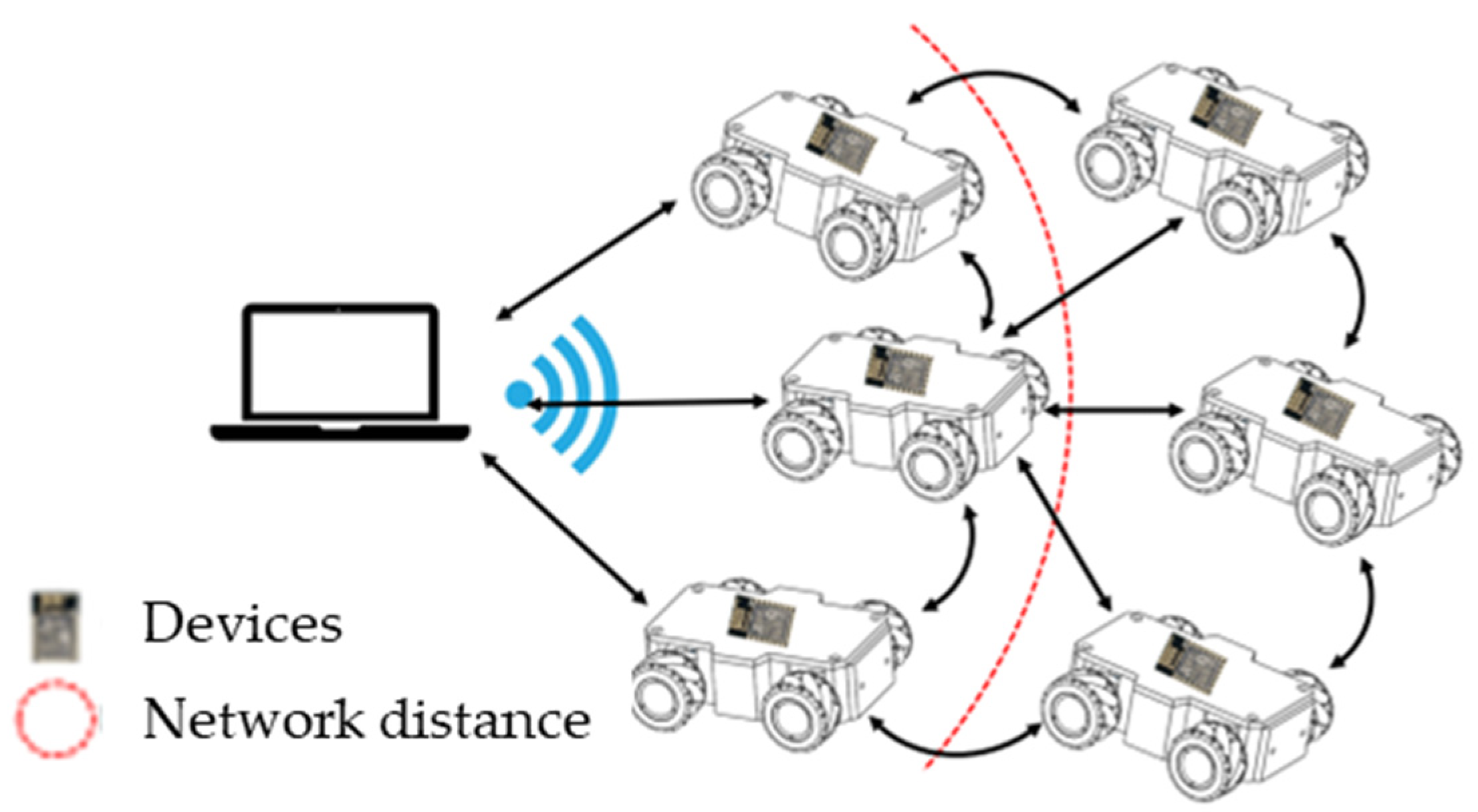
The ESP8266 module is used to complete the data transmission between the vehicle and the master computer. The ESP8266 has a set of network protocols (ESP-MESH) built on the basis of the WiFi protocol. It can form a self-organized network and is not limited by the distance between the central node and the device. In the reconfiguration system, using the ESP8266-MESH network protocol can enable the host computer to send commands to different modular vehicles in a multi-threaded manner, as shown in Figure 4.

3. UWB Positioning System

Acquiring the position of each vehicle is a prerequisite for reconfiguration. At present, the main indoor positioning methods mainly include computer vision [14], A-GPS (assisted GPS) [15], WiFi [16], Zigbee [17], UWB [18], etc.

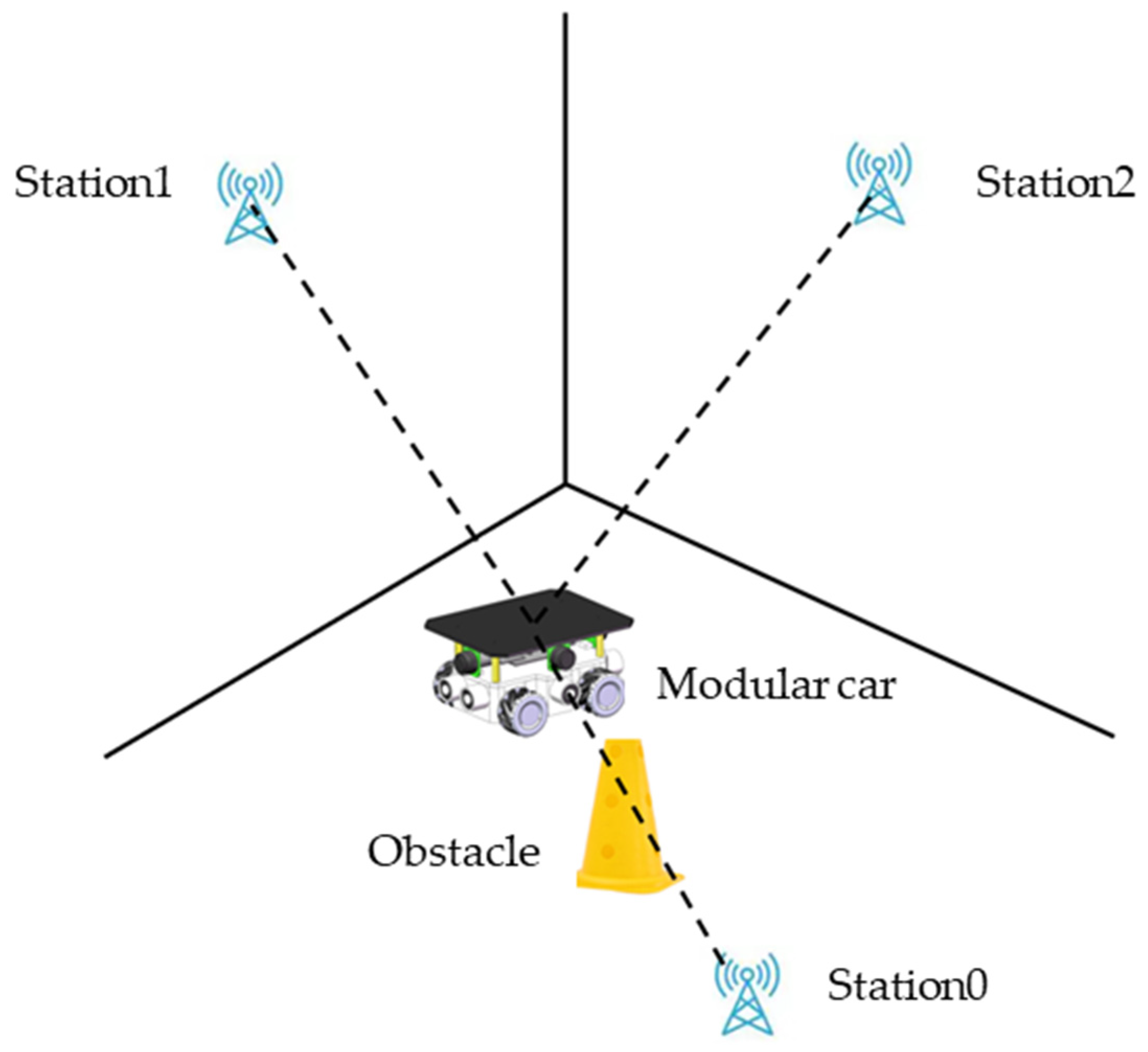
The modular vehicle positioning system based on UWB is shown in Figure 5. The system consists of positioning base stations and positioning tags on the vehicles. There are many obstacles in the room, such as load-bearing columns and furniture. Since the optical path is seriously blocked, it is inconvenient to use infrared positioning or visual positioning. Since the UWB system has good signal penetration, and since its base station can be placed at a high position, it cannot be affected by most obstacles, and it can achieve precise positioning and effective control of the self-reconfigurable modular vehicle.

In the UWB ranging system, the UWB signal is transmitted between the base station and the point to be located, and then the distance between the base station and the point is obtained. The two-way bilateral ranging method is used between the vehicle and the base station, as shown in Figure 6. According to Equation (1), the propagation time of the UWB signal can be calculated:

$$t_f=\frac{T_{round1}\ast T_{round2}-T_{reply1}\ast T_{reply2}}{T_{round1}+T_{round2}+T_{reply1}+T_{reply2}}$$

(1)

where t_f is the propagation time of the UWB signal, T_round1 is the time difference between the signal emitting time and the response receiving time in the vehicle, T_round2 is the time difference between the signal emitting time and the response receiving time in the station, T_reply1 is the response time in the station and T_reply2 is the response time in the vehicle.

Assuming that the clock drifts between the base station and that the modular vehicle are e_a and e_b, respectively, the error is:

$$error={\widehat{t}}_f-t_f=t_f\ast \frac{T_{reply1}(e_b{e}_a+e_a)*T_{reply2}(e_b{e}_a+e_b)}{T_{reply1}(1+e_a)+T_{reply2}(1+e_b)}$$

(2)

where ${\widehat{t}}_f$ is the absolute propagation time of the single UWB signal.

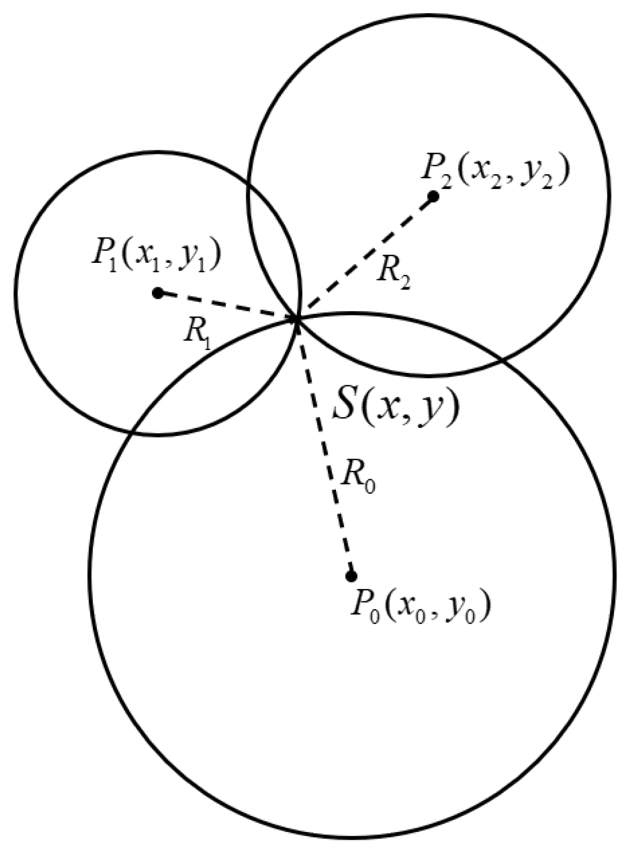
When the modular vehicle communicates with three base stations with the two-way bilateral method at the same time, the distance between the vehicle and the three base stations can be obtained, as shown in Figure 7. Among them, P₀(x₀,y₀), P₁(x₁,y₁) and P₂(x₂,y₂) are the coordinates of the three base stations in the UWB positioning system. S(x,y) is the label position of the modular vehicle. R₀, R₁ and R₂ are the absolute distances between the modular vehicle and the base station. The coordinates of the modular vehicle in the base station are obtained.

$$\left[\begin{array}{c}x\\ y\end{array}\right]={\left[\begin{array}{c}2(x_0-x_2)2(y_0-y_2)\\ 2(x_1-x_2)2(y_1-y_2)\end{array}\right]}^{-1}\times \left[\begin{array}{c}{x}_0^2-x_2^2+y_0^2-y_2^2+R_2^2-R_0^2\\ x_0^2-x_2^2+y_1^2-y_2^2+R_2^2-R_1^2\end{array}\right]$$

(3)

The UWB positioning system needs to ensure that all base stations are located in the same plane to reduce the distance error in the vertical direction when the vehicle communicates with the three base stations. The range of motion of the modular vehicle should be within the area surrounded by the three positioning base stations as close as possible; therefore, accurate positioning results can be obtained. If the vehicle is located at the edge of the positioning base station or within the range surrounded by the deviation base station, the positioning error may be large. When the modular vehicle exceeds the farthest ranging distance of the positioning base station, the UWB positioning system fails.

The UWB positioning system is mainly composed of a DW1000 chip and an STM32F103C8T6 chip. The UWB positioning label is placed in the middle of the vehicle, as shown in Figure 8a. The positioning system on the modular car realizes two-way bilateral data transmission with three positioning base stations. The distance between the modular car and the three positioning base stations is obtained by calculating the transmission time of the electromagnetic wave signal. Each positioning base station consists of a UWB signal antenna, UWB positioning module, support frame and 5 V power supply (Figure 8b). Since, in the whole positioning algorithm, each UWB positioning module transmits UWB electromagnetic wave signals through the UWB antenna, except base station 0 that needs to be connected to the upper computer, other base stations only need to send data back to base station 0 through radio signals.

4. Reconfiguration Path Planning Based on an Improved Artificial Potential Field Method

According to the input information of the vehicle, the path planning of the smart vehicle can be mainly divided into two categories: the global path planning that knows all the path and obstacle information, and the local path planning that only specifies the end point without inputting the obstacle information in advance. When working in a designated environment, it is necessary to store all obstacle sizes, map boundaries and their coordinate address information in advance. Then, the smart vehicle plans a specific route based on its own position and maps information with the goal of not colliding.

In local path planning, the vehicle does not know the location of obstacles in the path beforehand, but it relies on the sensors installed on the vehicle to detect the obstacles in the path in real time in the motion and according to the global path and obstacle information [19].

Global path planning has high requirements for data storage, data operation and the map modeling capabilities of a single vehicle, and information delay is likely to be caused when multiple modular vehicles are reconfigured. Considering that other modular vehicles also become dynamic obstacles during the reconfiguration process, it is more appropriate to use local path planning than global path planning.

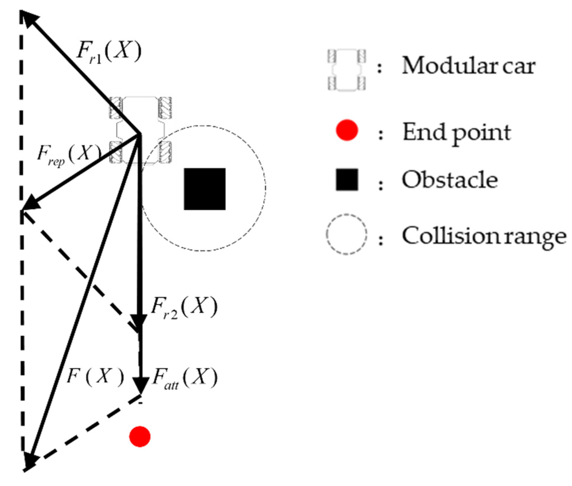
The artificial potential field method transforms the entire space into an artificial force field, sets the end point of the modular vehicle as the gravitational point and sets the obstacles on the reconfiguration path of the modular vehicle as the repulsive force point. Through the action of the potential field or the resultant force, the modular vehicle based on the artificial potential field method can move between its own position as the starting point and any position in space as the end point. Compared with the original artificial potential field, this improved method avoids the problem of falling into local optimal solutions.

The artificial potential field method is a virtual method proposed by Khatib to avoid the collision of the manipulator [20]. However, the traditional artificial potential field method has huge limitations when used for the reconfiguration of the modular vehicles. Therefore, the improved repulsion field function U_rep(x) is designed as:

$$U_{rep}(X)\{\begin{array}{l}\frac{1}{2}m{\left(\frac{1}{d}-\frac{1}{d_0}\right)}^2{d}_a{}^2,d\le d_0\\ 0,d>d_0\end{array}$$

(4)

The gravitational field function U_att(x) is designed as:

$$U_{att}(X)=\frac{1}{2}k\cdot d_a{}^2$$

(5)

Among them, X = (x,y) is the position of the modular vehicle; m is the repulsion gain coefficient; d is the distance between the modular vehicle and the obstacle; d₀ is the influence distance of the obstacle; d_a is the distance between the modular vehicle and the target reconfiguration point; and k is the gravitational gain coefficient.

According to the negative gradient, the repulsive force and the attractive force can be obtained, as shown in Figure 9.

$$F_{rep}(X)=\{\begin{array}{l}{F}_{r1}(X)+F_{r2}(X),d\le d_0\\ 0,d>d_0\end{array}$$

(6)

$$F_{r1}(X)=m\left(\frac{1}{d}-\frac{1}{d_0}\right)\frac{1}{d^2}{d}_a{}^2$$

(7)

$$F_{r2}(X)=-m{\left(\frac{1}{d}-\frac{1}{d_0}\right)}^2{d}_a$$

(8)

$$F_{att}(X)=-k\cdot d_a$$

(9)

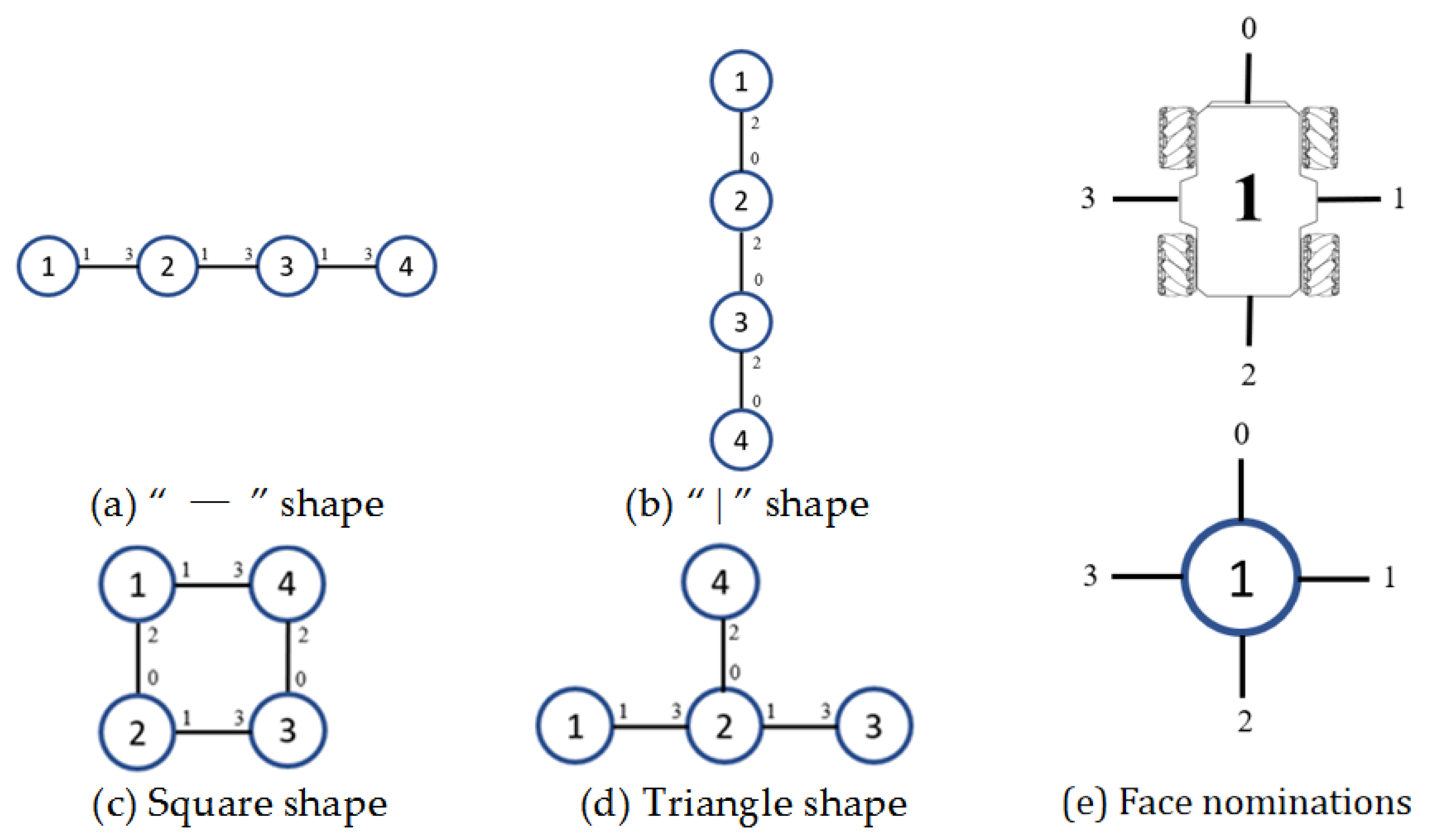
Considering the numbering of the magnetic device mentioned above, the four common configurations of modular vehicles and the connection relationship between the modular vehicles are shown in Figure 10, in which the number in the circle refers to the number of the vehicle, whereas the number outside the circle represents the connection face number. The nomination rule is explained in Figure 10e.

In order to describe the connection relationship between different configurations, a connection matrix C is defined, with a total of N rows and four columns, where each row represents a labeled modular vehicle, and each column represents the magnetic structure state corresponding to each modular vehicle:

$$C=\left[\begin{array}{cccc}{C}_{11}& C_{12}& C_{13}& C_{14}\\ C_{21}& C_{22}& C_{23}& C_{24}\\ & \dots & & \\ C_{n1}& C_{n2}& C_{n3}& C_{n4}\end{array}\right]$$

(10)

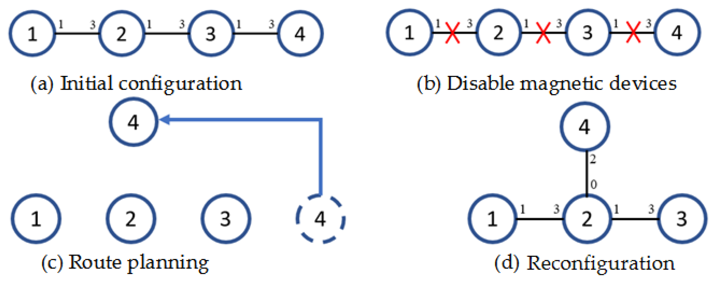
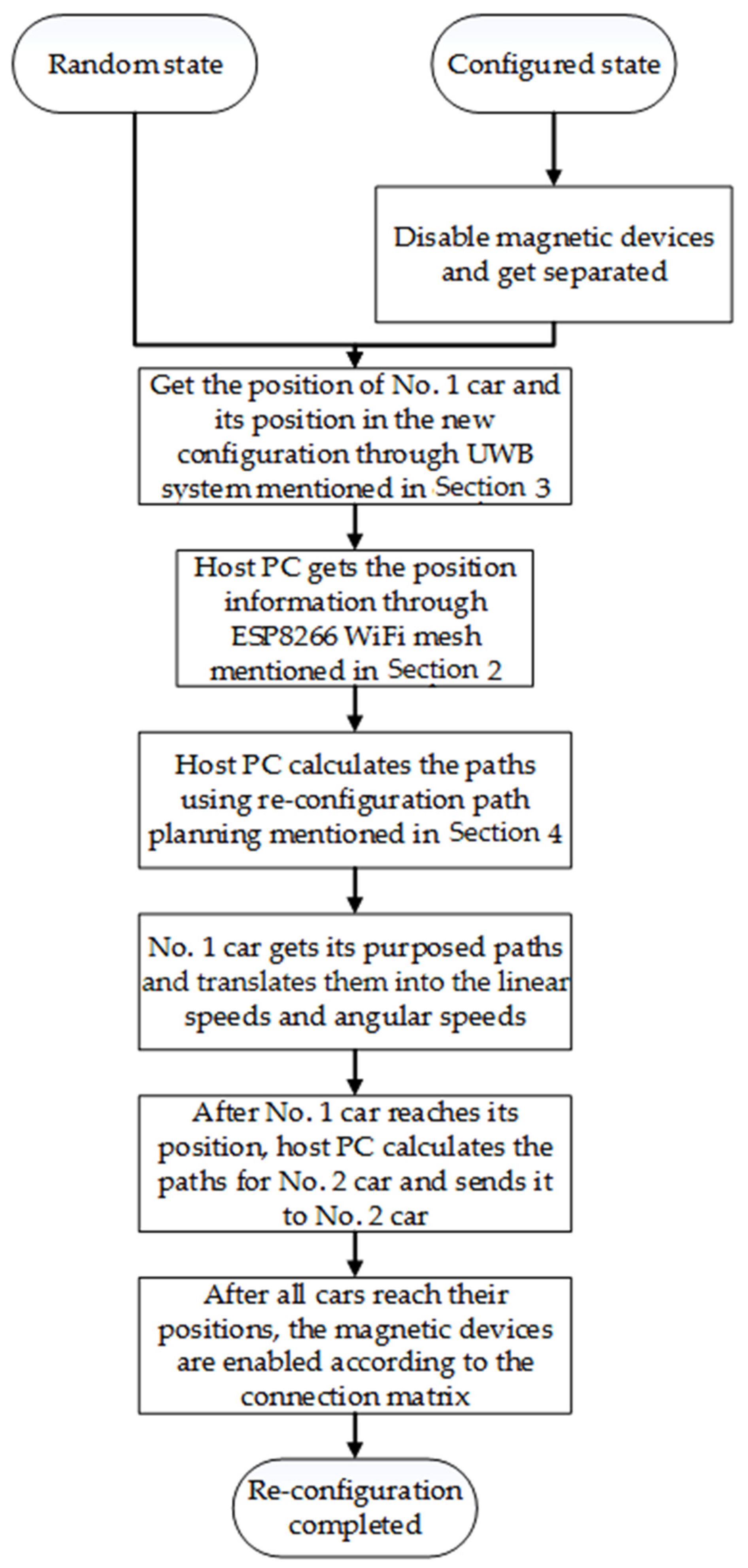
When the modular vehicle group is to be reconfigured, all magnetic structures are disabled, and then the UWB positioning system is used to obtain the position of the modular vehicle and the position of the target configuration. Local path planning based on the improved artificial potential field method is utilized to reach the target location. Finally, the connection matrix is sent to each modular car, thereby enhancing the stability of the configuration. The specific implementation process is shown in Figure 11.

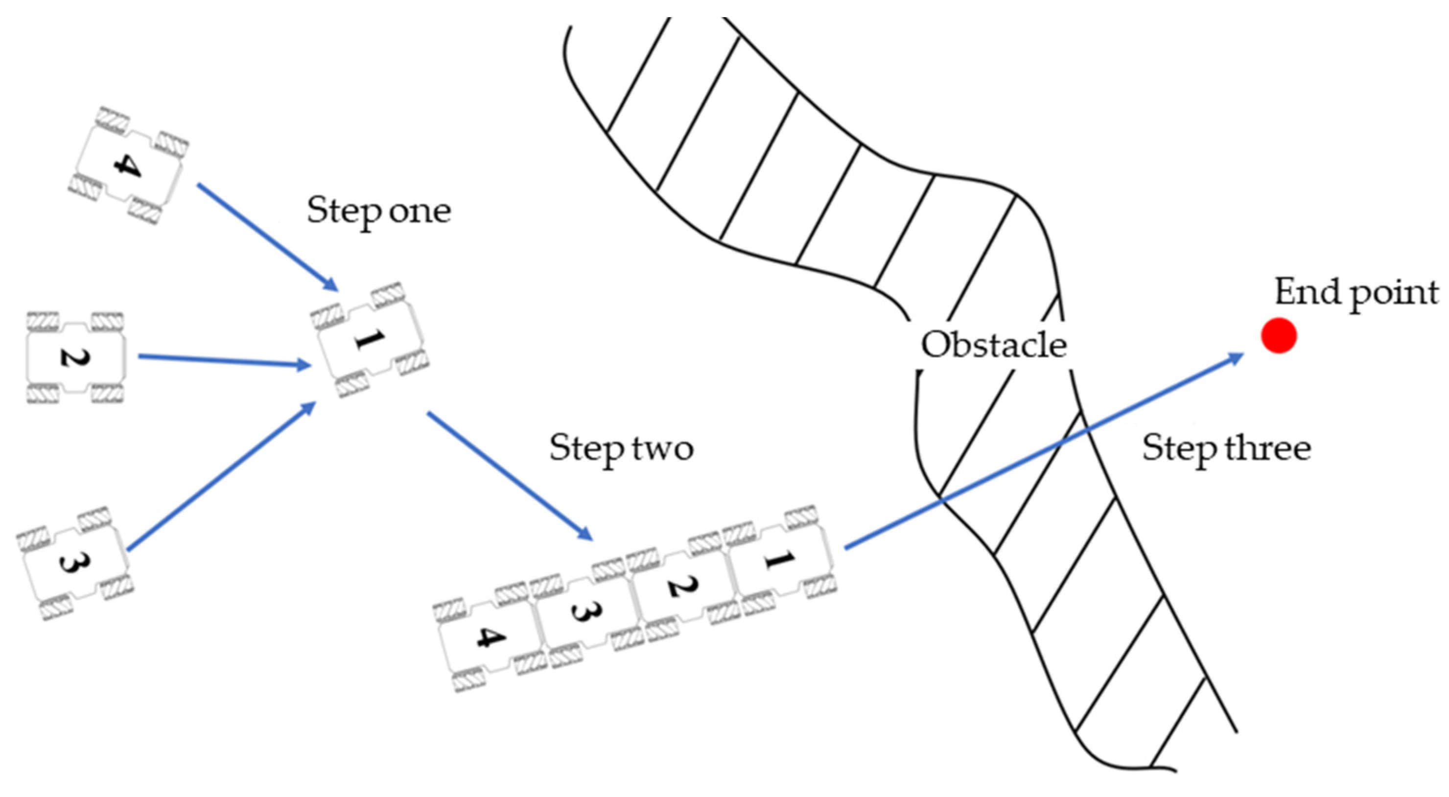
When the modular vehicle group encounters huge terrain obstacles (such as trenches), it can only be crossed by communicating with other modular vehicles and changing the configuration between the modular vehicles, as shown in Figure 12. In the first step, the pilot’s modular vehicle detects the obstacles. Through the UWB positioning system, the host computer obtains the spatial coordinates of the modular vehicle. In the second step, the master computer sends the target coordinates of other modular vehicles according to the target configuration, and the modular vehicle performs path planning and reconfiguration according to the improved artificial potential field method. In the third step, each modular vehicle receives coordinated instructions to enable the group to cross obstacles.

The whole algorithm process and its implementation are shown in Figure 13.

5. Simulation and Experiment

5.1. UWB Positioning and WiFi Communication Experiment

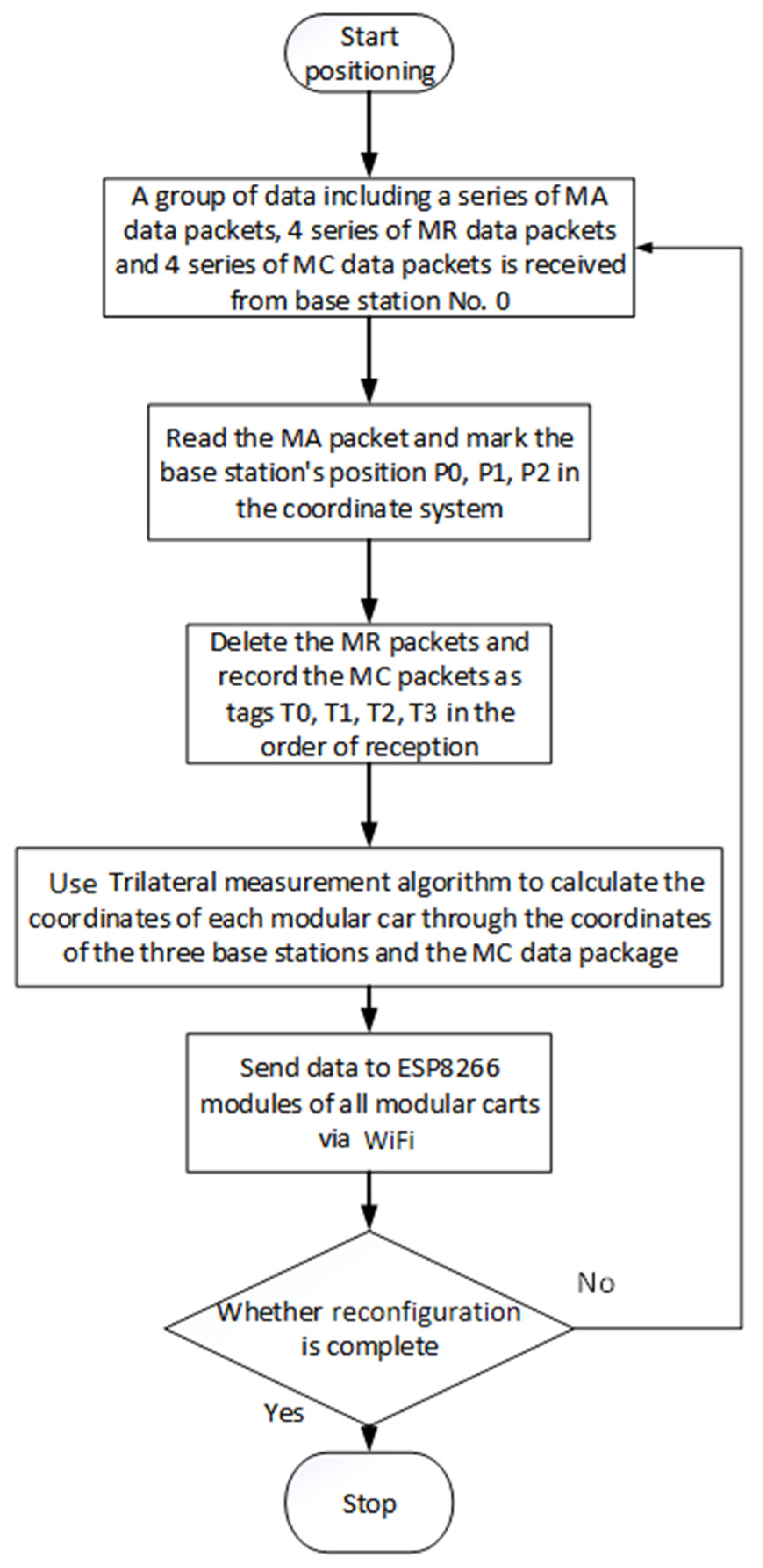
To implement the UWB positioning system, the coordinates of the three positioning base stations need to be acquired, and then two-way bilateral communication is used to calculate the distance between the vehicle positioning tag and each positioning base station. After obtaining the straight-line distances between two base stations and between the base station and the positioning tag, a trilateration algorithm is used to calculate the coordinates of the modular vehicle. The UWB positioning algorithm flow is shown in Figure 14, in which MA data represent the distance between the different base stations, which is used for the positioning between the base stations and the establishment of the coordinate system. The MR data represent the original distance data between the tag and the base station, and the MC data represent the optimized and corrected distance between the tag and the base station, which is used for tag positioning.

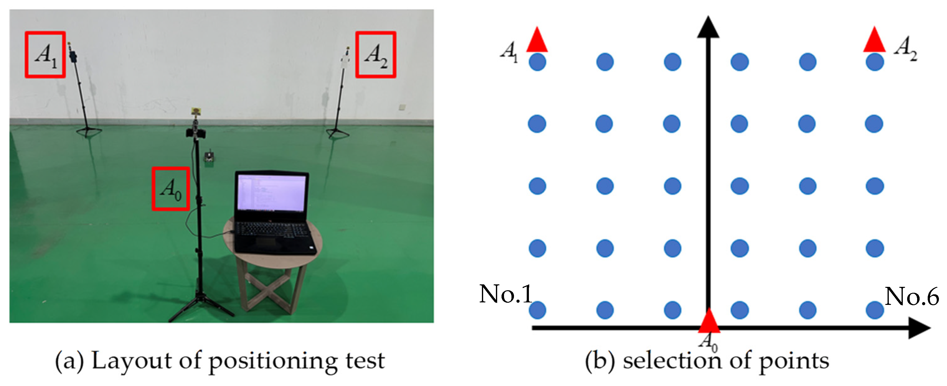
In order to verify the accuracy of UWB positioning on the modular vehicle group, three positioning base stations are used indoors to form a 3 × 3 m² square area. The coordinates of the three base stations are A₀(0, 0), A₁(−1.5, 3) and A₂(1.5, 3), as shown in Figure 15a. The selection of the positioning points of the modular vehicle is shown in Figure 15b, and the selection of the positioning points divides the entire plane into 30 positioning points. The interval between each positioning points is 0.6 m, as shown by blue dots in Figure 15b.

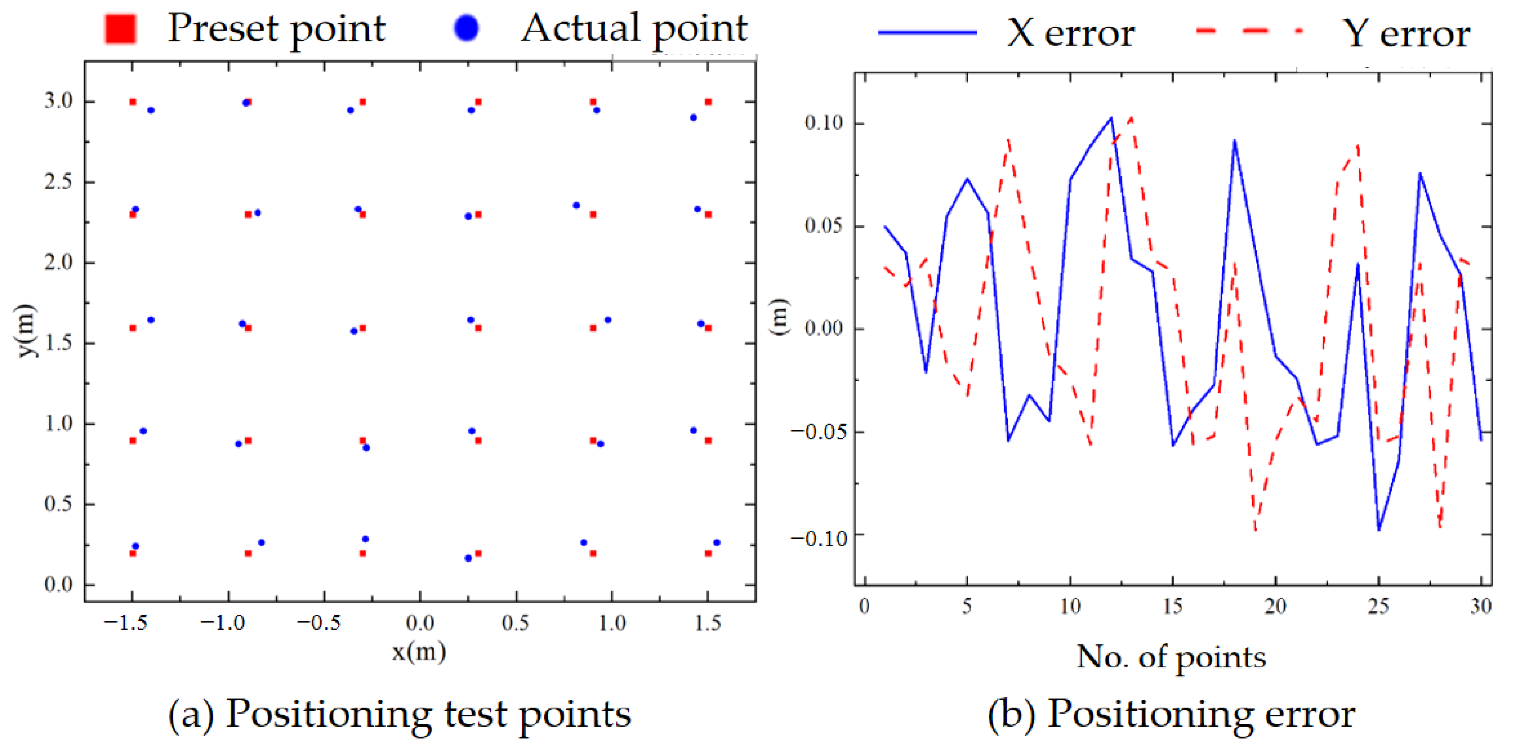
The average value of ten positioning data is taken as the measurement value at each point, and the measurement result is shown in Figure 16a. The errors of the horizontal and vertical coordinates (x and y) of the actual sampling point in Figure 16a and the coordinates of the measured positioning point are calculated, respectively, as shown in Figure 16b, where it can be seen that the accuracy of the UWB-based modular vehicle positioning system can be up to ±0.1 m.

Stable, low-latency communication ensures the performance of the modular vehicle. Each modular vehicle is given a unique fixed IP address. The WiFi configuration of the modular vehicle is numbered as 1, its IP address is set to 172.20.10.1 and the IP address of the host computer is set to 172.20.10.5. The ESP8266 WiFi Mesh is shown in Algorithm 1.

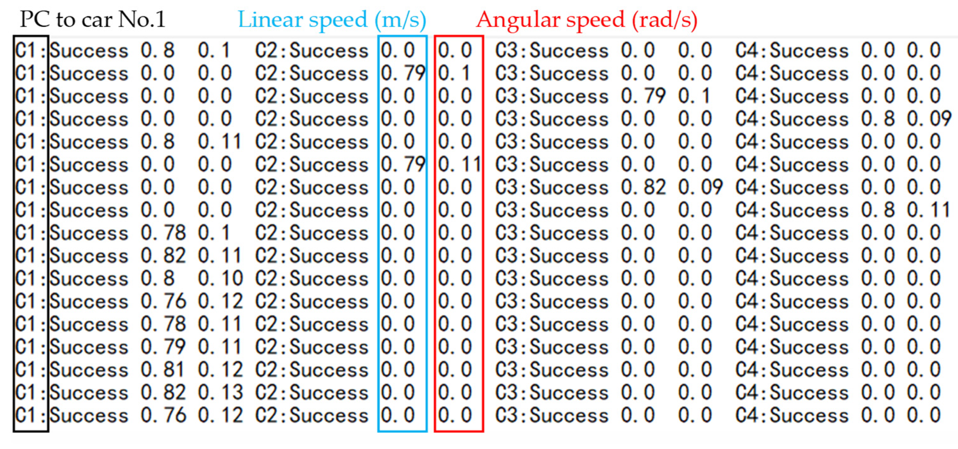
Each modular vehicle is connected to the local network to send and receive data. The master computer sends the speed and angular velocity required by each modular vehicle to the ESP8266 module, as shown in Figure 17. The ESP8266 module on the modular vehicle then sends the speed information to the main control chip.

Algorithm 1 ESP8266 WiFi Mesh

Includes: ESP8266WiFi.h ESP8266WiFiMesh.h assert.h   Statements: *ssid *password IP subnet et.al   function SetupWiFi.persistent()   Serial.begin()   Serial.printIn()   meshNode.activateAP()   function Mainloop

5.2. Simulation of Modular Vehicle Reconfiguration

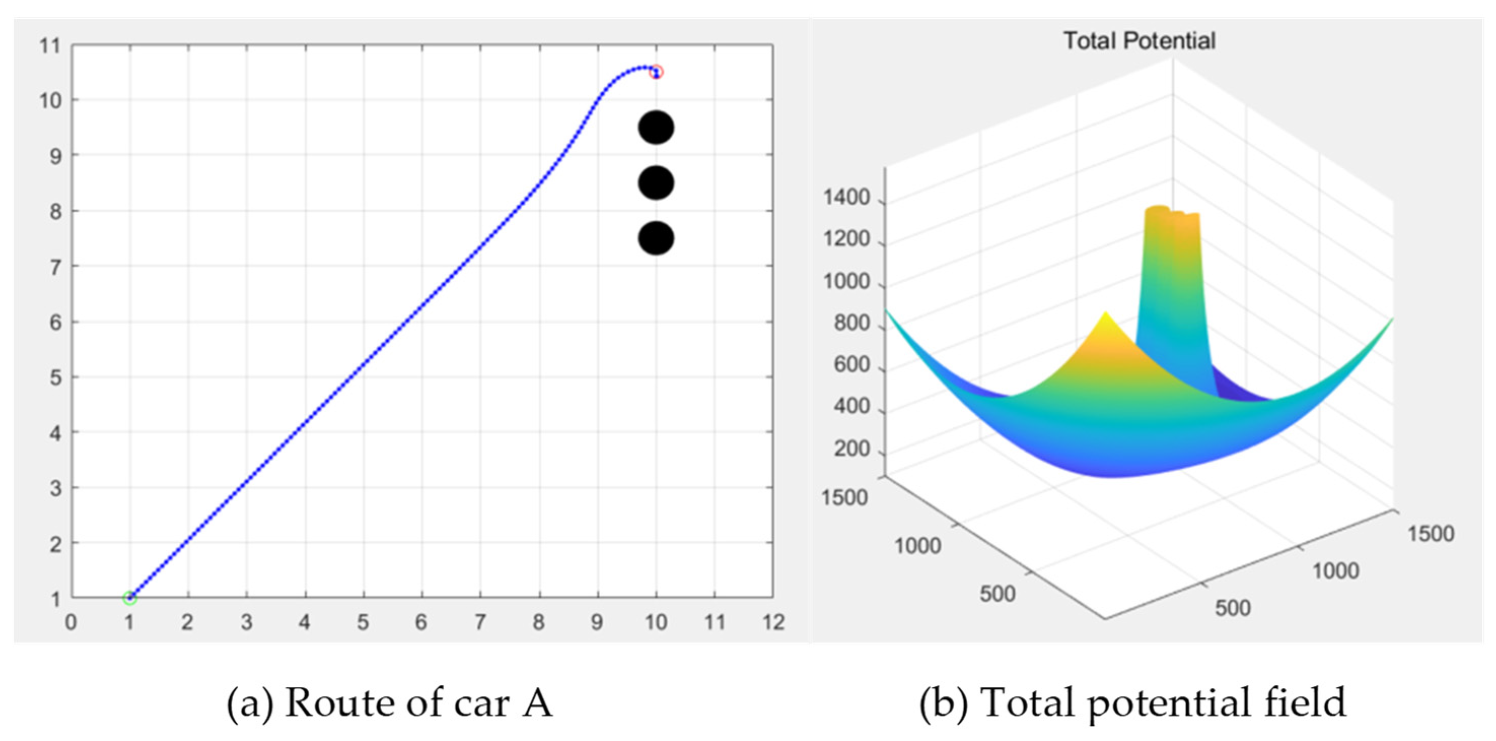
Based on the path planning algorithm mentioned above, the reconfiguration of the modular vehicle is simulated. Assuming that there is a group consisting of four modular vehicles, in which modular vehicles B, C and D have reached their positions, their initial positions are B (10, 9.5), C (10, 8.5) and D (10, 7.5). The gravitational gain coefficient is set to be 28, the repulsive force gain coefficient is set to be 25, the influence range of the repulsive potential field regarded as an obstacle is 5, the simulation step size is 0.1 s, the maximum acceleration is 1 m/s², the maximum speed is 1 m/s and the modular vehicle A starts from the start point (1, 1) towards the target point (10, 10). The local path planning performed utilizing the artificial potential field method is shown in Figure 18a. The repulsive potential formed by modular vehicles B, C and D field is shown in Figure 18b.

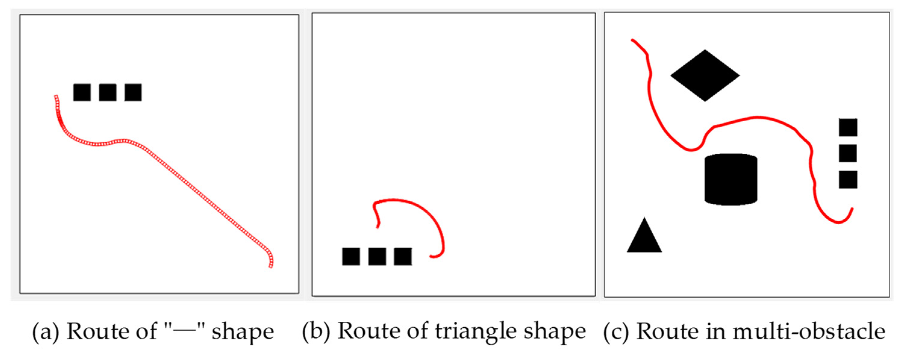
Under the same simulation parameters, the “—” shape configuration simulation route for a single modular vehicle is shown in Figure 19a, and the triangular configuration simulation route for a single modular vehicle is shown in Figure 19b. When the modular vehicle is in a complex multi-obstacle environment, its path route is as that which is shown in Figure 19c.

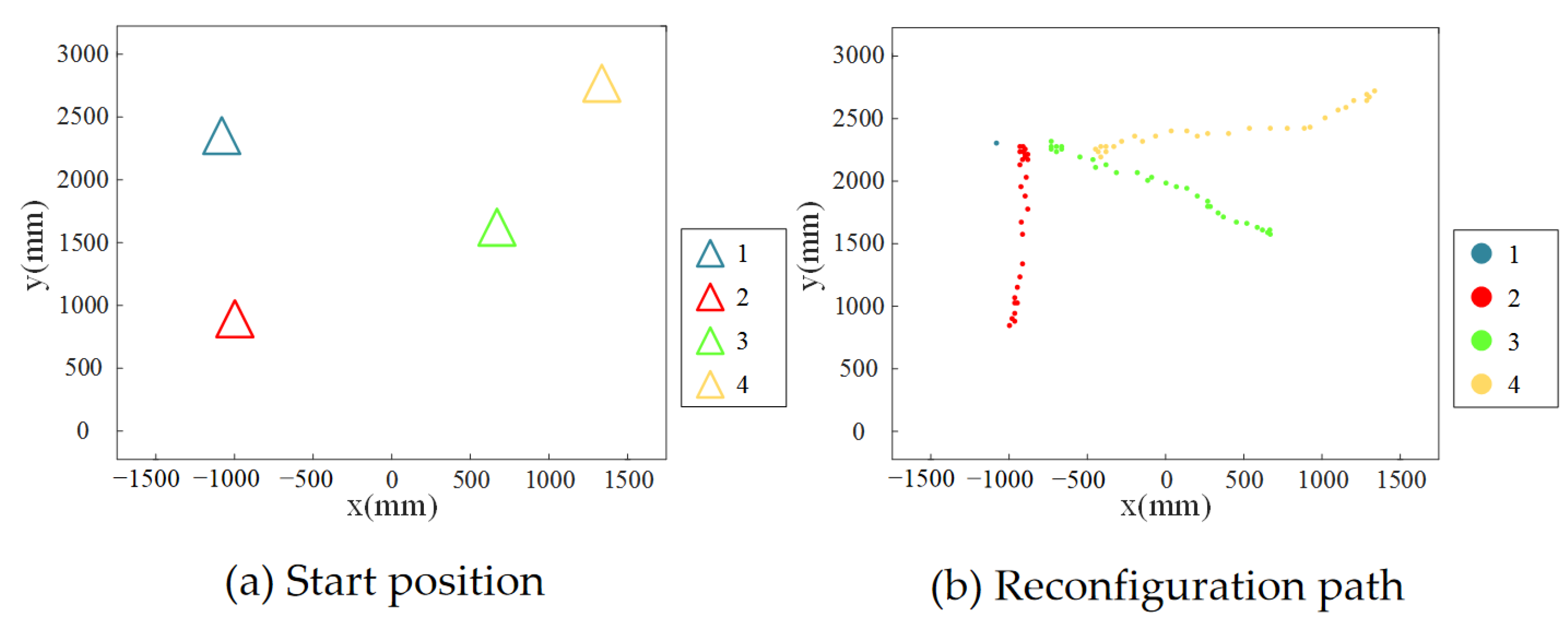
During the reconfiguration process of the modular vehicle group, only one modular vehicle performs the path planning at each moment. The latter modular vehicle regards the previous one that has completed the path planning as an obstacle that needs to be avoided and performs path planning according to the improved artificial potential field method to reach the designated target point until all modular vehicles are reconfigured, and the host computer broadcasts the connection matrix to the modular vehicle. The modular vehicle enables the magnetic device according to the connection matrix, and a complete reconfiguration process ends. Supposing that the state of the modular vehicle group is as that which is shown in Figure 20, in order to realize the reconfiguration of the “ | “ shape, when the No. 2 modular vehicle approaches the No. 1 modular vehicle, the rest of the vehicles are regarded as obstacles, and the path is as that which is shown in Figure 20. When the No. 3 modular vehicle approaches the No. 2 modular vehicle, the rest of the vehicles are regarded as obstacles. When the No. 4 modular vehicle approaches, the rest of the vehicles are regarded as obstacles. The initial positions and reconfiguration paths of the four modular vehicles in the above reconfiguration process are placed in the same diagram, as shown in Figure 20.

5.3. Experiment of Modular Vehicle Reconfiguration

5.3.1. “—” Shape Reconfiguration

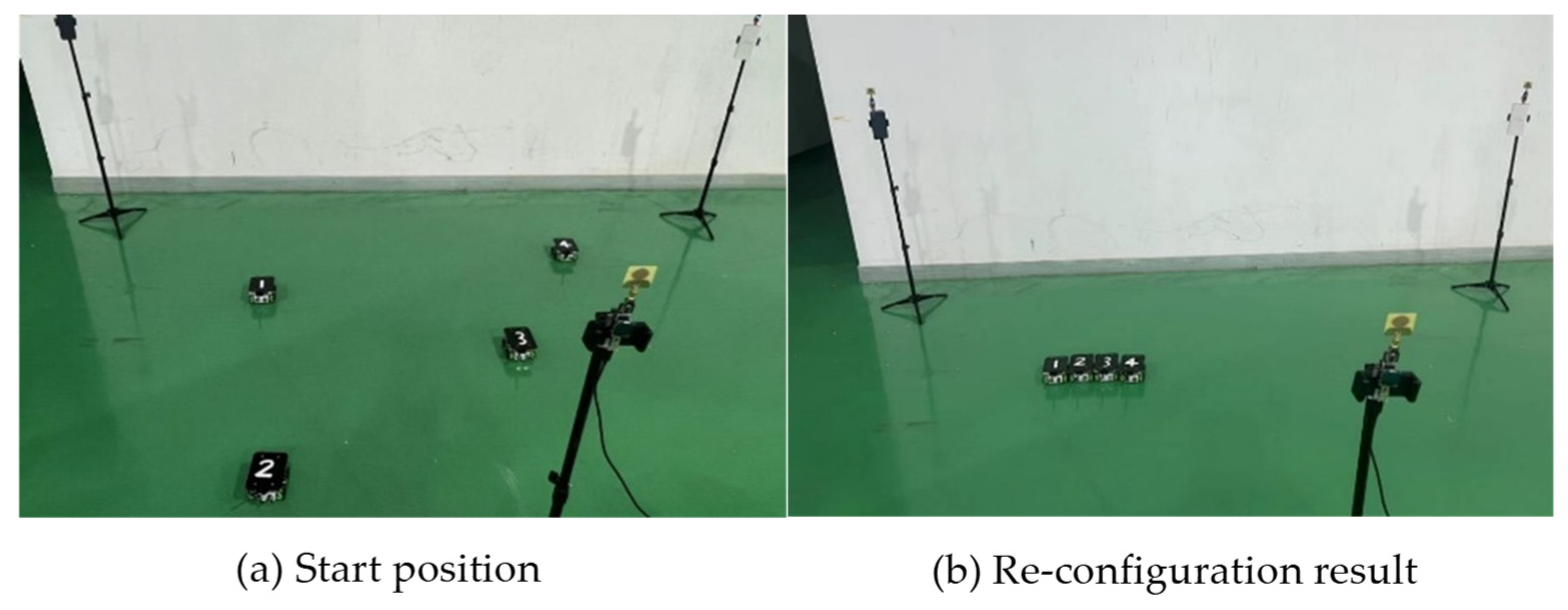
Figure 21 shows the visualization result of the “—” shape reconfiguration of the modular vehicle group and Figure 22 shows the “—” shape reconfiguration procedure. During the process, the position of the No. 1 modular vehicle remains unchanged, and the host computer performs path planning for the No. 2 modular vehicle and sends the speed and angular velocity data to the No. 2 modular vehicle. At the beginning, the moving speed of the modular vehicle is fast, and when approaching the end point, the moving speed slows down. After the No. 2 modular vehicle moves to the corresponding position, the host computer sends control commands to the No. 3 modular vehicle and the No. 4 modular vehicle in the same way. Finally, a magnetic device is used to bring the four modular vehicles into a stable configuration. The detailed information can be found in supplementary materials video S1.

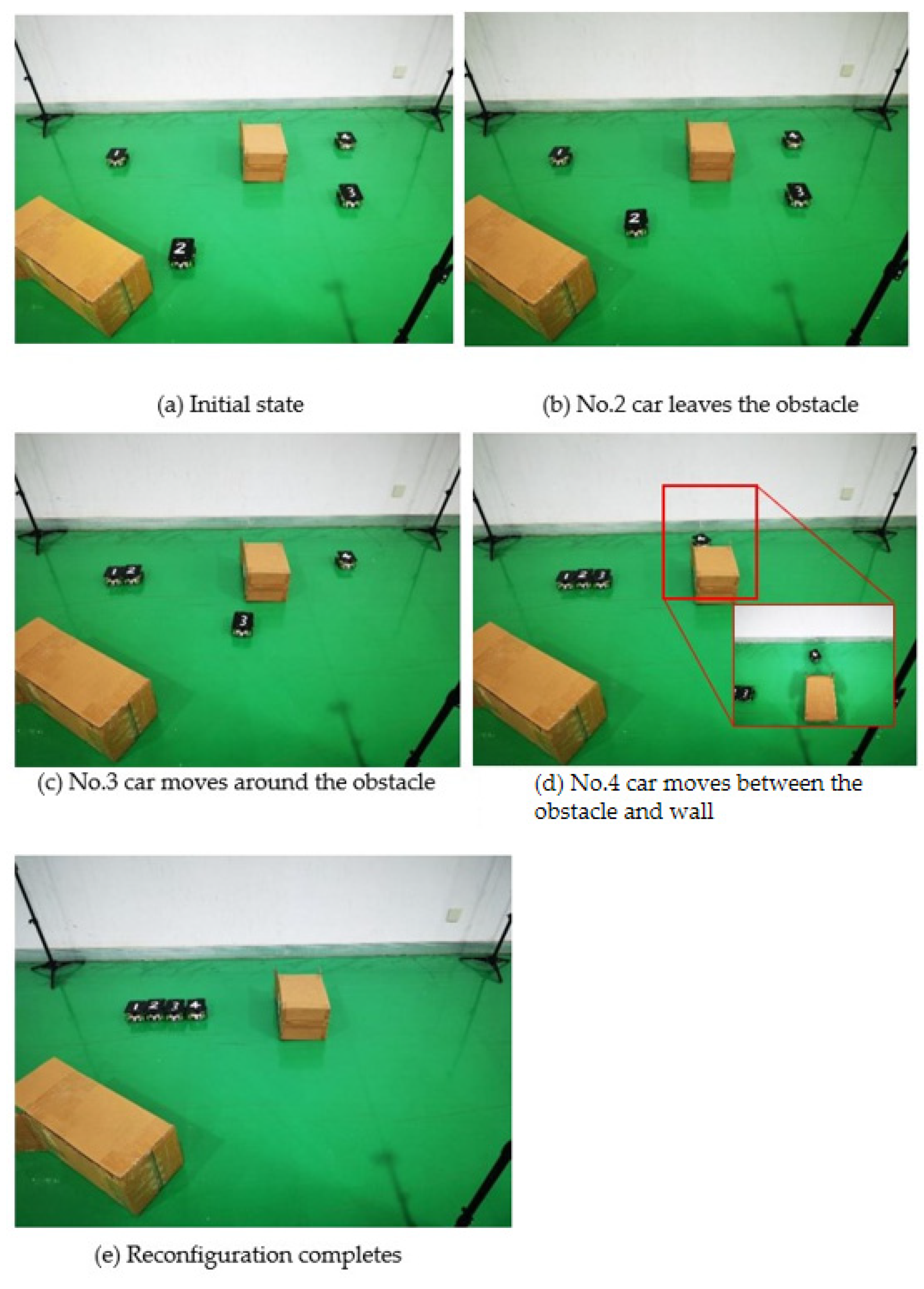
In the “—”-shaped reconfiguration with obstacles, the specific process is as follows (Figure 23). Car No. 1 is set as the reference point and remains stationary. Car No. 2 is too close to the obstacle and is affected by the repulsive force. It moves away from the obstacle object until it is out of the influence distance of the obstacle, and then it goes straight to the target coordinates. Vehicle No. 3 is interfered by an obstacle on the forward path, and it moves approximately along the obstacle-affected distance. The distance between the wall and the obstacle is greater than two times the influence distance of the obstacle, so the No. 4 vehicle passes between the wall and the obstacle to reach the designated position.

5.3.2. “|” Shape Reconfiguration

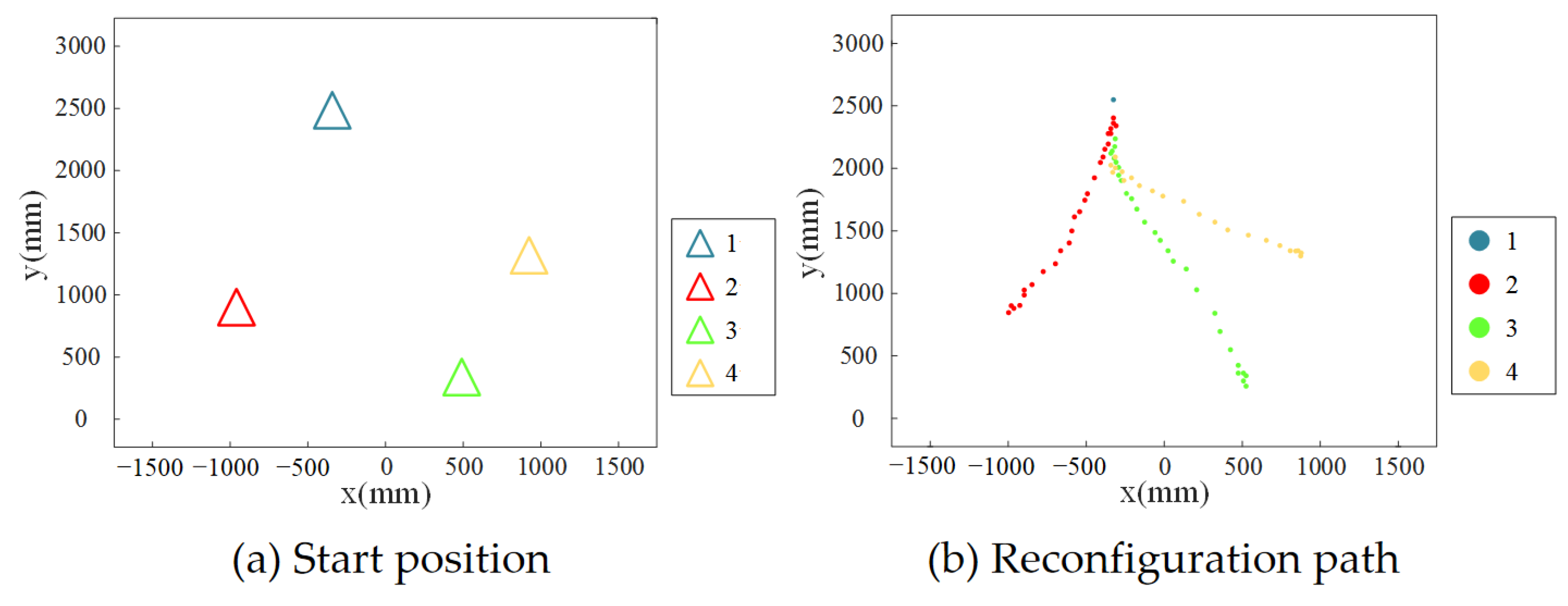
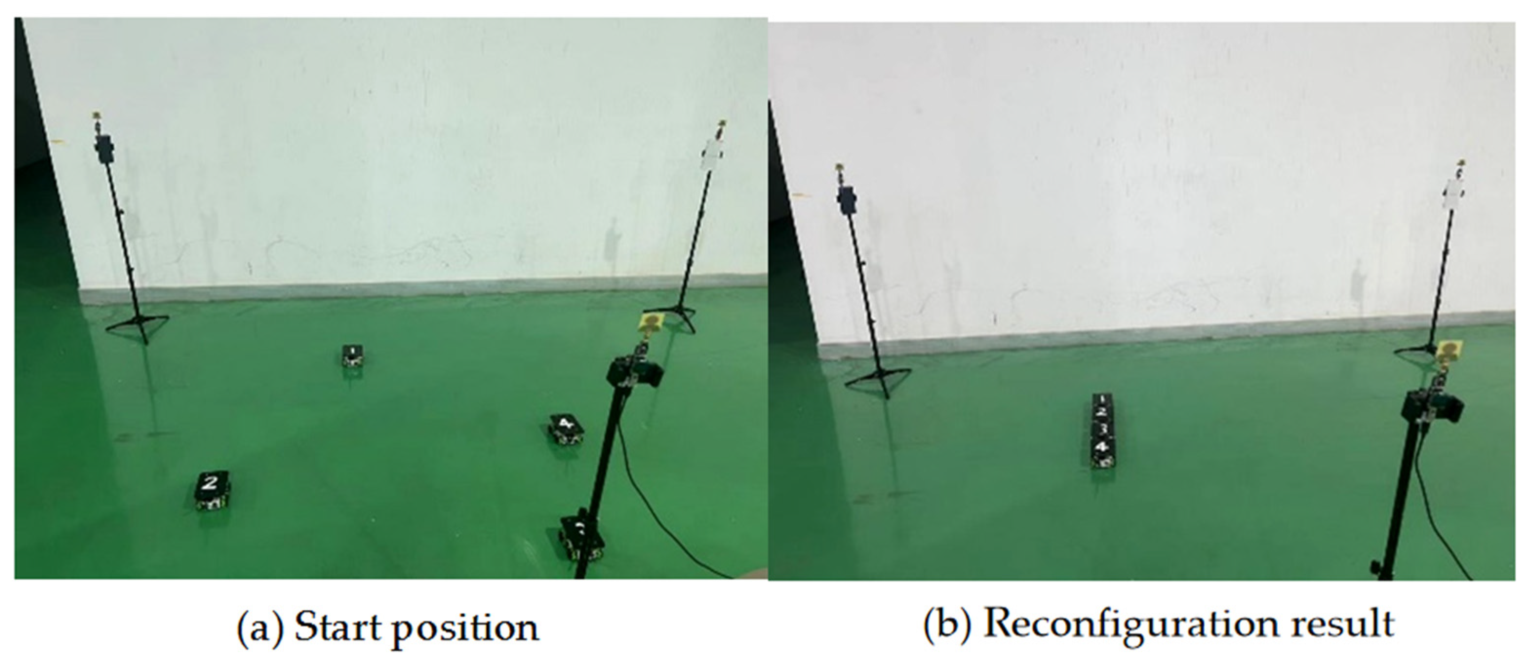
Figure 24 shows the visualization results of the modular vehicle group “|” shape reconfiguration and Figure 25 shows the “|” shape reconfiguration procedure. The modular vehicle group is in the initial random state, and through the UWB positioning system, each modular vehicle completes the reconfiguration of the “|” shape after the path planning movement of the target point. The detailed information can be found in supplementary materials video S2.

5.3.3. Transformation between the Two Configurations

To test the adaptability of the modular vehicle to different tasks and usage environments, a reconfiguration experiment of the modular vehicle from one configuration to another is designed. The initial state of the modular vehicle group is in the “—” shape, as shown in Figure 26.

The reconfiguration process is shown in Figure 27. At the beginning, the magnetic structures on all modular vehicles are disabled. The No. 1 modular vehicle separates from the original configuration and moves toward the target point, when the other modular vehicles are regarded as obstacles. After the No. 1 modular vehicle reaches its target point, the No. 4 modular vehicle starts to depart from the original configuration and moves towards its target point. After all the modular vehicles reach their target point, each vehicle enables the magnetic structure according to the connection matrix to ensure the stability of the configuration.

5.4. Results and Discussion

The error analysis is carried out on the reconfiguration process of the “—” shape of the modular vehicles. After the modular vehicle stops moving, the error between the actual distance and the expected distance is used to evaluate the reconfiguration accuracy. After several reconfiguration movements, the distance is manually measured and averaged. The results are shown in

Table 1. Actual distance of modular vehicles with “—” shape.

The Relationship	1–2	2–3	3–4
X-axis distance/mm	121.3	118.2	119.8
Y-axis distance/mm	6.3	7.2	5.5

.

After 20 reconstructions, the distances between the vehicles are measured and averaged before the magnets are enabled, as shown in

Table 2. Actual distance of modular vehicles with “|” shape.

The Relationship	1–2	2–3	3–4
X-axis distance/mm	6.8	5.4	7.3
Y-axis distance/mm	149.8	148.6	151.2

.

The distance between the X axis and the Y axis represents the offset distance between the two centers of the adjacent vehicles. The length of the vehicle on the X axis and the Y axis is 110 mm × 140 mm.

Table 3. Reconfiguration speed.

	“—” Shape	“|” Shape	“⊥” Shape
Reconfiguration times	20	20	30
Success rate	95% (19/20)	100% (20/20)	93% (28/30)
Average time	1 min. 30 s.	1 min. 18 s.	1 min. 41 s.

gives the experimental results of the reconfiguration of the proposed strategy with four modular vehicles.

In Table 3, reconfiguration success is defined as: when each sub-module vehicle correctly enables the magnetic device according to the connection matrix, the vehicle itself does not have a large deviation. The average time is calculated as the average time for all successful reconfiguration experiments. All experiments start from the disorderly dispersed state of the sub-module vehicle and end with the completion of the overall configuration.

The “|” shape configuration is relatively easy. The success rate is high, and the average time is short. The “—” shape configuration takes a longer time because of the lateral translation of the Mecanum wheel. The “⊥” shape configuration is more complicated, and the fusion of the “|” shape configuration and the “—” shape configuration needs to be considered in the reconfiguration process.

The modular vehicle group in the simulation and experiment are composed of four vehicles. However, the proposed reconfiguration strategy is static in its steps and dynamic as a whole, i.e., the path planning of the reconfiguration process is composed of the individual reconfiguration path planning of each vehicle. The next vehicle starts only when the previous vehicle completes the reconfiguration. When the number of vehicles increases, the group reconstruction time increases, but the reconfiguration complexity does not increase significantly. This enables the proposed strategy to scale well to groups consisting of more vehicles.

Due to the limitations of application scenarios, logistics vehicles usually run on the plane. Therefore, this paper only considers the planer solution with three base stations. However, the 3D solution with more base stations is certainly a promising perspective, which deserves further research work.

6. Conclusions

This paper proposes a reconfigurable control strategy for reconfigurable modular vehicles. Using the multi-sensor self-positioning Mecanum vehicle designed in this paper, through the UWB bilateral two-way ranging and triangulation algorithm, taking the selected position as the end point and using the improved artificial potential field method, different reconfiguration paths are carried out for each modular vehicle in the group. Finally, the reconfiguration experiment of the modular vehicle is carried out, and the reconfiguration process from the “—” shape to the “|” shape is realized. The experimental results show that the hardware setting and control algorithm of the self-reconfigurable modular vehicle proposed in this paper are feasible, robust and scalable, and the reconfiguration process has high execution precision. Modular vehicles can form different configurations according to different applications, which greatly improves the adaptability of intelligent vehicle systems.