Article

Adaptive Fuzzy Control for Flexible Robotic Manipulator with a Fixed Sampled Period

School of Electrical, Electronics and Computer Science, Guangxi University of Science and Technology, Liuzhou 545000, China
*
Author to whom correspondence should be addressed.
Electronics 2022, 11(14), 2270; https://doi.org/10.3390/electronics11142270
Submission received: 23 June 2022 / Revised: 8 July 2022 / Accepted: 19 July 2022 / Published: 20 July 2022

Abstract

:
In this paper, a backstepping sampled data control method is developed for a flexible robotic manipulator whose internal dynamic is completely unknown. To address the internal uncertainties, the fuzzy logical system (FLS) is considered. Moreover, considering the limited network bandwidth, the designed controller and adaptive laws only contain the sampled data with a fixed sampled period. By invoking the Lyapunov stability theory, all signals of the flexible robotic manipulator are semi-global uniformly ultimately bounded (SGUUB). Ultimately, an application to a flexible robotic manipulator is given to verify the validity of the sampled data controller.

1. Introduction

For the past few years, robotics has experienced rapid development and has become widely used in a variety of fields, such as military, industry, aerospace and so on. With the thriving of robotics, the flexible robotic manipulator has also attracted wide attention, and diverse interesting control methods are being investigated, such as sliding control [1,2,3,4,5], feedback linearization method [6,7], and the passivity approach [8,9]. It should be noticed that modeling errors are inevitable in the actual modeling process, which will bring about a certain deviation in the dynamic characteristics of the model. Therefore, in order to allow the proposed method to be better applied in practice, the internal dynamics of the flexible robotic manipulator in this paper are considered unknown. To estimate the internal dynamics of the flexible robotic manipulator, the fuzzy logical system (FLS) is considered under the backstepping structure.
Recently, a number of backstepping adaptive fuzzy controllers have been designed subject to the flexible robotic manipulator [10,11,12,13,14,15,16,17,18,19,20]. In [18], by transforming the single-link flexible robotic manipulator system with unknown internal dynamics into an uncertain fifth-order nonlinear system, a backstepping adaptive fuzzy controller was developed for the fifth-order transformation model. However, it should be noticed that there exists an “explosion of complexity” problem in [18], which is mainly caused by the repeated appearance of the time derivative of virtual control signals. In [19], by introducing error compensation signals, a command filter is designed to conquer the “explosion of complexity” problem. In this paper, FLS is used to approximate the time derivative of virtual control signals to avert the “explosion of complexity” problem, which simplifies the backstepping structure and is more suitable for the practical case.
Along another key line of research, as a result the limit of the network bandwidth in practice, plenty of adaptive sampled data control approaches have been developed [20,21,22,23,24,25,26]. Rather than the normal adaptive fuzzy control method in [10,11,12,13,14,15,16,17,18,19,20], the difficulty of sampling control is mainly reflected in two aspects. Firstly, in order to save more network bandwidth, the network will transmit data after a fixed sampling period, which means the backstepping sampled data control method can only use the information at the sampling time. Secondly, there always exist errors between the sampled data and the continuous data. How to ensure the stability of controlled objects by only using sampling data is a significant problem. Especially, under the backstepping structure, sampled data will be used in each step, which increases the difficulty of stability analysis.
In this paper, an adaptive fuzzy backstepping sampled data control method is developed subject to a flexible robotic manipulator. Firstly, by transforming the flexible robotic manipulator into a fifth-order non-strict feedback nonlinear system and using FLS to approximate the nonlinear function, the sampled data controller is designed. On the basis of Gronwall–Bellman inequality and Lyapunov stability theory, the designed sampled-data controller can guarantee that all closed-loop signals are semi-globally uniformly ultimately bounded (SGUUB). The main contributions are summarized below:
(1)
This paper is the first work concerning adaptive fuzzy backstepping sampled-data control for a flexible robotic manipulator system. In the control process, the designed controller only needs the sampled information of states rather the continuous case.
(2)
By using the property of the fuzzy basic function, the algebraic loop issue caused by the non-strict feedback system is avoided. Furthermore, the designed adaptive laws also consider the sampled data, which is a great difference from previous works.

2. Preliminaries and Problem Formulation

The dynamics equation of a single-link manipulator with brushless direct current (DC) motor based on non-rigid joints is shown below [19]:
J 1 q ¨ 1 + F 1 q ˙ 1 + K ( q 1 q 2 N ) + M g d cos q 1 = 0 J 2 q ¨ 2 + F 2 q ˙ 2 K N ( q 1 q 2 N ) = K a I L I ˙ + R I + K c q ˙ 2 = u
where J 1 and J 2 are the inertia coefficients, F 1 and F 2 are the viscous friction constants, K is the spring coefficient, M is the link mass, g is the acceleration of gravity, d is the center of gravity of the link, N is the gear ratio, K a is the torque coefficient, I is the current of the armature, R is the armature resistance, L is the armature inductance, K c is the back electromotive force constant, u is the armature voltage, and q 1 and q 2 are the angular position of the connecting rod and the motor shaft, respectively.
For the sake of applying the backstepping structure for a single-link flexible joint robot model (1), define the conversion variables as x 1 = q 1 , x 2 = q ˙ 1 , x 3 = q 2 , x 4 = q ˙ 2 , and x 5 = I . Thus, model (1) can be rewritten as
x ˙ 1 = x 2 x ˙ 2 = f 1 ( x 1 , x 2 , x 3 ) + x 3 x ˙ 3 = x 4 x ˙ 4 = f 2 ( x 1 , x 3 , x 4 , x 5 ) + x 5 x ˙ 5 = f 3 ( x 4 , x 5 ) + u L
where f 1 ( x 1 , x 2 , x 3 ) = F 1 J 1 x 2 K J 1 ( x 1 x 3 N ) M g d J 1 cos x 1 x 3 , f 2 ( x 1 , x 3 , x 4 , x 5 ) = F 2 J 2 x 4 + K J 2 N ( x 1 x 3 N ) + K a J 2 x 5 x 5 and f 3 ( x 4 , x 5 ) = R L x 5 K c L x 4 .
In this paper, to effectively reduce the burden of network bandwidth, the sampled data control method has been considered. The armature voltage u only needs to be updated at the sampling time. To state the concept clearly, another signal υ is introduced to reflect the continuous change of the armature voltage u . In the subsequent calculation, the system states can only be obtained from the sampled data, which brings an enormous challenge to the analysis of the stability under the backstepping structure.
Before giving the control objective, the following preparations of FLS are first presented.
Lemma 1 
[18]. If f ( x ) is a continuous function of a compact set  Ω , then for a constant ε > 0 , the FLS θ T φ ( x )  satisfies
sup x Ω | f ( x ) θ T φ ( x ) | ε
where  ε  is the fuzzy minimum approximation error, and there exists a positive constant ε  that satisfies  | ε | ε ;  θ T = [ θ 1 , θ 2 , , θ N ] is desired parameter vector of FLS, and φ ( x ) = [ φ 1 ( x ) , , φ N ( x ) ] T  is defined as
φ l = i = 1 n μ F i l ( x i ) l = 1 N ( i = 1 n μ F i l ( x i ) )
Control Objective: The control objective of this work is to design an adaptive sampled-data control strategy for transformation model (2) by utilizing the sampled data of the states. Under the Lyapunov stability theory, all closed-loop signals are proved to converge a small residual set.

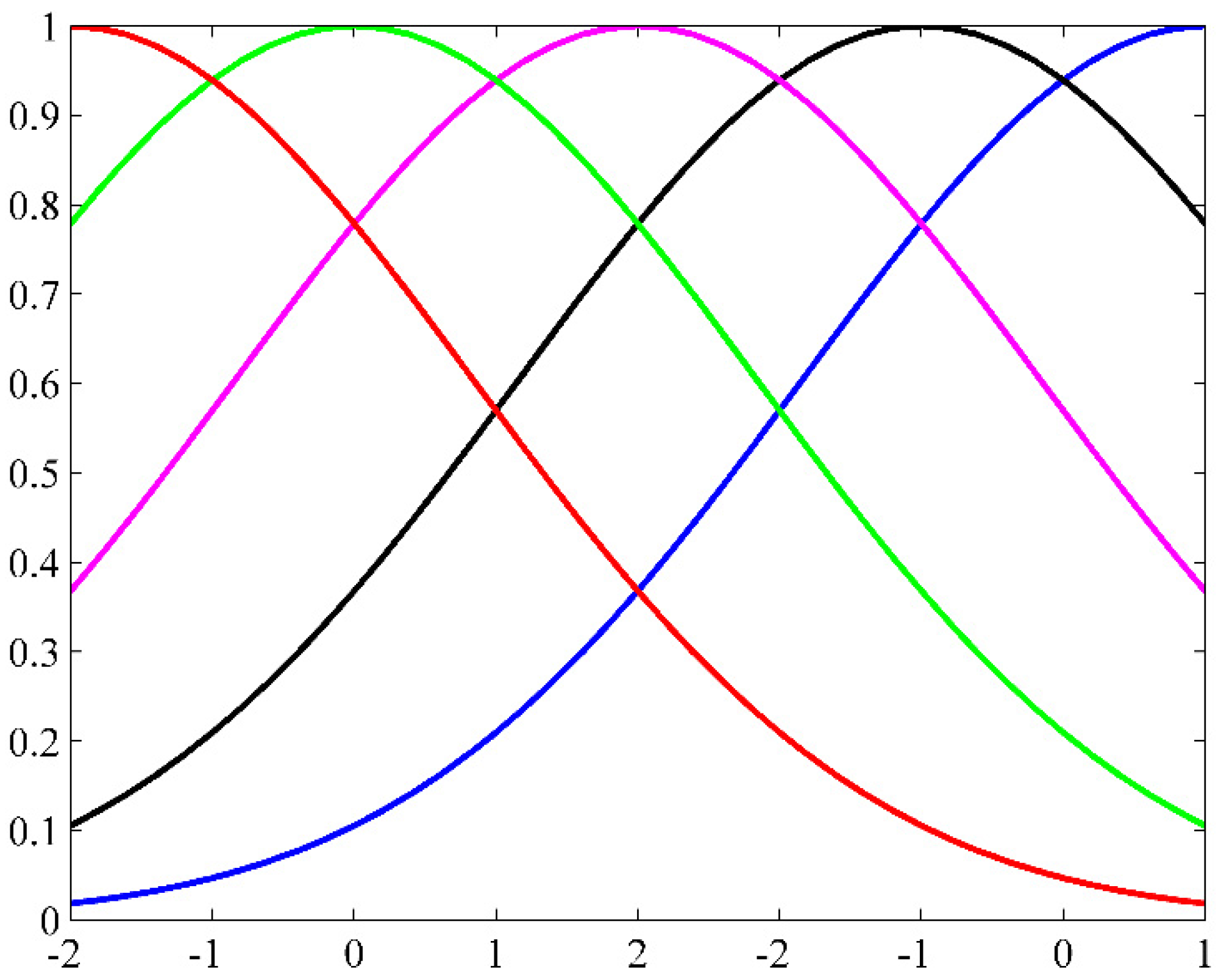
3. Adaptive Fuzzy Controller Design and Stability Analysis

In this section, an adaptive fuzzy sampled-data controller is designed for the backstepping structure, and the stability of the closed-loop system is proved by Lyapunov function stability theory.
In the first place, to design the adaptive sampled-data controller, the coordinate changes under the backstepping structure are defined as
z 1 ( t ) = x 1 ( t ) , z i ( t ) = x i ( t ) α i 1 ( i = 2 , 3 , 4 , 5 )
where α i 1 is the virtual control signal specified. To simplify the expression of the formula, we denote z j ( j = 1 , 2 , 3 , 4 , 5 ) and x j as z j ( t ) and x j ( t ) , respectively.
As the sampled-data controller is only formed from the state at the sampling time, the adaptive fuzzy controller design process is divided into two parts. In case 1, we design the sampled-data controller and analyze the stability in the time interval ( t k , t k + 1 ) , where the time sequence t k denotes the k - t h sampling activity. In case 2, we analyze the stability at the sampling time t k .
Case 1.
Step 1. To design the sampled-data controller for transformation model (2), we chose the Lyapunov function as
V 1 = 1 2 z 1 2
On the basis of the designed coordinate changes (4) and Lyapunov function (5), the time derivative of Lyapunov function can be expressed as
V ˙ 1 = z 1 ( z 2 + α 1 )
By applying Young’s inequality, one can obtain
z 1 z 2 1 2 z 1 2 + 1 2 z 2 2
For the backstepping structure, we design the virtual control signal α 1 as
α 1 = c 1 z 1 1 2 z 1
Substituting (7) and (8) into (6) yields
V ˙ 1 c 1 z 1 2 + 1 2 z 2 2
Step 2. In Step 2, we design the Lyapunov function as
V 2 = V 1 + 1 2 z 2 2 + 1 2 θ ˜ 1 T θ ˜ 1
where θ ˜ 1 = θ 1 θ ^ 1 is the approximation error between the ideal FLS parameter vector θ 1 and its estimation variable θ ^ 1 .
In accordance with the Lyapunov function (10), its time derivative form can be expressed as
V ˙ 2 c 1 z 1 2 + 1 2 z 2 2 + z 2 ( f 1 ( x 1 , x 2 , x 3 ) + z 3 + α 2 α ˙ 1 ) θ ˜ 1 T θ ^ ˙ 1
By utilizing Lemma 1 to approximate the function g 1 ( x 1 , x 2 , x 3 ) = f 1 + c 1 x 2 + 1 2 x 2 , one has
V ˙ 2 c 1 z 1 2 + 1 2 z 2 2 + z 2 ( z 3 + α 2 + θ 1 T φ 1 ( x 1 , x 2 , x 3 ) + ε 1 + θ 1 T φ 1 ( x 1 ( t k ) , x 2 ( t k ) ) θ 1 T φ 1 ( x 1 ( t k ) , x 2 ( t k ) ) ) θ ˜ 1 T θ ^ ˙ 1
Using Young’s inequality and the property of the fuzzy basic function 0 < φ 1 T ( ) φ 1 ( ) 1 , we can obtain
z 2 z 3 + z 2 θ 1 T φ 1 ( x 1 , x 2 , x 3 ) z 2 2 + 1 2 θ 1 T θ 1 + 1 2 z 3 2
z 2 θ 1 T φ 1 ( x 1 ( t k ) , x 2 ( t k ) ) + z 2 ε 1 z 2 2 + 1 2 θ 1 T θ 1 + 1 2 ε 1 2
Substituting (13) and (14) into (12) leads to
V ˙ 2 z 2 ( α 2 + θ ^ 1 T φ 1 ( x 1 ( t k ) , x 2 ( t k ) ) + θ ˜ 1 T φ 1 ( x 1 ( t k ) , x 2 ( t k ) ) ) θ ˜ 1 T θ ^ ˙ 1 + 5 2 z 2 2 + θ 1 T θ 1 + 1 2 ε 1 2 + 1 2 z 3 2 c 1 z 1 2
We design the virtual control signal and adaptive law for Step 2 as
α 2 = c 2 z 2 θ ^ 1 T φ 1 ( x 1 ( t k ) , x 2 ( t k ) ) 5 2 z 2
θ ^ ˙ 1 = z 2 ( t k ) φ 1 ( x 1 ( t k ) , x 2 ( t k ) ) δ 1 θ ^ 1
Substituting (16) and (17) into (15) results in
V ˙ 2 ( z 2 z 2 ( t k ) ) θ ˜ 1 T φ 1 ( x 1 ( t k ) , x 2 ( t k ) ) + δ 1 θ ˜ 1 T θ ^ 1 + θ 1 T θ 1 + 1 2 ε 1 2 + 1 2 z 3 2 c 1 z 1 2 c 2 z 2 2
Based on Young’s inequality, we further have
( z 2 ( t k ) z 2 ) θ ˜ 1 T φ 1 ( x 1 ( t k ) , x 2 ( t k ) ) + δ 1 θ ˜ 1 T θ ^ 1 1 4 ( z 2 z 2 ( t k ) ) 2 + ( 1 δ 1 2 ) θ ˜ 1 T θ ˜ 1 + δ 1 2 θ 1 T θ 1
The time derivative of Lyapunov function can be rewritten as
V ˙ 2 1 2 z 3 2 c 1 z 1 2 c 2 z 2 2 + 1 4 ( z 2 z 2 ( t k ) ) 2 + ( 1 δ 1 2 ) θ ˜ 1 T θ ˜ 1 + d 1
where d 1 = ( 1 + δ 1 2 ) θ 1 T θ 1 + 1 2 ε 1 2 .
Step 3. In accordance with Step 2, we take the Lyapunov function as
V 3 = V 2 + 1 2 z 3 2 + 1 2 θ ˜ 2 T θ ˜ 2
where θ ˜ 2 = θ 2 θ ^ 2 is the approximation error between the ideal FLS parameter vector θ 2 and its estimation variable θ ^ 2 .
Recalling the definition of the coordinate changes (4), the time derivative of (21) can be represented as
V ˙ 3 1 2 z 3 2 c 1 z 1 2 c 2 z 2 2 + 1 4 ( z 2 z 2 ( t k ) ) 2 + ( 1 δ 1 2 ) θ ˜ 1 T θ ˜ 1 + d 1 + z 3 ( x 4 α ˙ 2 ) θ ˜ 2 T θ ^ ˙ 2
To avoid using the time derivative of the virtual control signal, the FLS is considered to approximate the α ˙ 2 , which yields
V ˙ 3 1 2 z 3 2 c 1 z 1 2 c 2 z 2 2 + 1 4 ( z 2 z 2 ( t k ) ) 2 + ( 1 δ 1 2 ) θ ˜ 1 T θ ˜ 1 + d 1 θ ˜ 2 T θ ^ ˙ 2 + z 3 ( z 4 + α 3 + θ 2 T φ 2 ( x 1 , x 2 , x 3 ) + ε 2 + θ 2 T φ 2 ( x 1 ( t k ) , x 2 ( t k ) , x 3 ( t k ) ) θ 2 T φ 2 ( x 1 ( t k ) , x 2 ( t k ) , x 3 ( t k ) ) )
Invoking Young’s inequality and the property of the fuzzy basic function 0 < φ 2 T ( ) φ 2 ( ) 1 , one has
z 3 z 4 + z 3 θ 2 T φ 2 ( x 1 , x 2 , x 3 ) z 3 2 + 1 2 θ 2 T θ 2 + 1 2 z 4 2
z 3 θ 2 T φ 2 ( x 1 ( t k ) , x 2 ( t k ) , x 3 ( t k ) ) + z 3 ε 2 z 3 2 + 1 2 θ 2 T θ 2 + 1 2 ε 2 2
Substituting (24) and (25) into (23), one can have
V ˙ 3 5 2 z 3 2 c 1 z 1 2 c 2 z 2 2 + 1 4 ( z 2 z 2 ( t k ) ) 2 + ( 1 δ 1 2 ) θ ˜ 1 T θ ˜ 1 + d 1 θ ˜ 2 T θ ^ ˙ 2 + θ 2 T θ 2 + 1 2 z 4 2 + z 3 ( α 3 + θ 2 T φ 2 ( x 1 ( t k ) , x 2 ( t k ) , x 3 ( t k ) ) ) + 1 2 ε 2 2
Design the virtual control signal and adaptive law as
α 3 = c 3 z 3 θ ^ 2 T φ 2 ( x 1 ( t k ) , x 2 ( t k ) , x 3 ( t k ) ) 5 2 z 3
θ ^ ˙ 2 = z 3 ( t k ) φ 2 ( x 1 ( t k ) , x 2 ( t k ) , x 3 ( t k ) ) δ 2 θ ^ 2
Substituting (27) and (28) into (26), we can obtain
V ˙ 3 i = 1 3 c i z i 2 + 1 4 ( z 2 z 2 ( t k ) ) 2 + ( 1 δ 1 2 ) θ ˜ 1 T θ ˜ 1 + d 1 θ ˜ 2 T θ ^ ˙ 2 + θ 2 T θ 2 + 1 2 z 4 2 ( z 3 ( t k ) z 3 ) θ ˜ 2 T φ 2 ( x 1 ( t k ) , x 2 ( t k ) , x 3 ( t k ) ) + δ 2 θ ˜ 2 T θ ^ 2 + 1 2 ε 2 2
Using Young’s inequality, the following inequality holds:
( z 3 ( t k ) z 3 ) θ ˜ 2 T φ 2 ( x 1 ( t k ) , x 2 ( t k ) , x 2 ( t k ) ) + δ 2 θ ˜ 2 T θ ^ 2 1 4 ( z 3 z 3 ( t k ) ) 2 + ( 1 δ 2 2 ) θ ˜ 2 T θ ˜ 2 + δ 2 2 θ 2 T θ 2
In accordance with (29) and (30), one has
V ˙ 3 i = 1 3 c i z i 2 + 1 4 i = 2 3 ( z i z i ( t k ) ) 2 + i = 1 2 ( 1 δ i 2 ) θ ˜ i T θ ˜ i + d 2 + 1 2 z 4 2
where d 2 = ( 1 + δ 2 2 ) θ 2 T θ 2 + 1 2 ε 2 2 .
Step 4. In this step, we consider the Lyapunov function as
V 4 = V 3 + 1 2 z 4 2 + 1 2 θ ˜ 3 T θ ˜ 3
where θ ˜ 3 = θ 3 θ ^ 3 is the approximation error between the ideal FLS parameter vector θ 3 and its estimation variable θ ^ 3 .
Then, the time derivative of (32) can be easily calculated as
V ˙ 4 i = 1 3 c i z i 2 + 1 4 i = 2 3 ( z i z i ( t k ) ) 2 + i = 1 2 ( 1 δ i 2 ) θ ˜ i T θ ˜ i + d 2 + 1 2 z 4 2 + z 4 ( f 2 ( x 1 , x 3 , x 4 , x 5 ) + z 5 + α 4 α ˙ 3 ) θ ˜ 3 T θ ^ ˙ 3
To eliminate the impact of the nonlinear function f 2 ( x 1 , x 3 , x 4 , x 5 ) and the time derivative of virtual control signal α ˙ 3 , it can be further obtained that
V ˙ 4 i = 1 3 c i z i 2 + 1 4 i = 2 3 ( z i z i ( t k ) ) 2 + i = 1 2 ( 1 δ i 2 ) θ ˜ i T θ ˜ i + d 2 + 1 2 z 4 2 + z 4 ( z 5 + α 4 + θ 3 T φ 3 ( x 1 , x 2 , x 3 , x 4 , x 5 ) + ε 3 + θ 3 T φ 3 ( x 1 ( t k ) , x 2 ( t k ) , x 3 ( t k ) , x 4 ( t k ) ) θ 3 T φ 3 ( x 1 ( t k ) , x 2 ( t k ) , x 3 ( t k ) , x 4 ( t k ) ) ) θ ˜ 3 T θ ^ ˙ 3
Then, invoking Young’s inequality and the property of the fuzzy basic function 0 < φ 3 T ( ) φ 3 ( ) 1 again, we obtain
z 4 z 5 + z 4 θ 3 T φ 3 ( x 1 , x 2 , x 3 , x 4 , x 5 ) z 4 2 + 1 2 θ 3 T θ 3 + 1 2 z 5 2
z 4 θ 3 T φ 3 ( x 1 ( t k ) , x 2 ( t k ) , x 3 ( t k ) , x 4 ( t k ) ) + z 4 ε 3 z 4 2 + 1 2 θ 3 T θ 3 + 1 2 ε 3 2
By inserting (35) and (36) into (34), it is not difficult to obtain
V ˙ 4 i = 1 3 c i z i 2 + 1 4 i = 2 3 ( z i z i ( t k ) ) 2 + i = 1 2 ( 1 δ i 2 ) θ ˜ i T θ ˜ i + d 2 + 5 2 z 4 2 + θ 3 T θ 3 + 1 2 z 5 2 + 1 2 ε 3 2 + z 4 ( α 4 + θ 3 T φ 3 ( x 1 ( t k ) , x 2 ( t k ) , x 3 ( t k ) , x 4 ( t k ) ) ) θ ˜ 3 T θ ^ ˙ 3
Thereafter, we configure the virtual control signal and adaptive law as
α 4 = c 4 z 4 θ ^ 3 T φ 3 ( x 1 ( t k ) , x 2 ( t k ) , x 3 ( t k ) , x 4 ( t k ) ) 5 2 z 4
θ ^ ˙ 3 = z 4 ( t k ) φ 3 ( x 1 ( t k ) , x 2 ( t k ) , x 3 ( t k ) , x 4 ( t k ) ) δ 3 θ ^ 3
Substituting the virtual control signal (38) and adaptive law (39) into (37) gives
V ˙ 4 i = 1 4 c i z i 2 + 1 4 i = 2 3 ( z i z i ( t k ) ) 2 + i = 1 2 ( 1 δ i 2 ) θ ˜ i T θ ˜ i + d 2 + θ 3 T θ 3 + 1 2 ε 3 2 ( z 4 ( t k ) z 4 ) θ ˜ 3 T φ 3 ( x 1 ( t k ) , x 2 ( t k ) , x 3 ( t k ) , x 4 ( t k ) ) + δ 3 θ ˜ 3 T θ ^ 3
Based on Young’s inequality, the following inequality holds:
( z 4 ( t k ) z 4 ) θ ˜ 3 T φ 3 ( x 1 ( t k ) , x 2 ( t k ) , x 3 ( t k ) , x 4 ( t k ) ) + δ 3 θ ˜ 3 T θ ^ 3 1 4 ( z 4 z 4 ( t k ) ) 2 + ( 1 δ 3 2 ) θ ˜ 3 T θ ˜ 3 + δ 3 2 θ 3 T θ 3
Combining (29) and (30) gives
V ˙ 4 i = 1 4 c i z i 2 + 1 4 i = 2 4 ( z i z i ( t k ) ) 2 + i = 1 3 ( 1 δ i 2 ) θ ˜ i T θ ˜ i + d 3 + 1 2 z 5 2
where d 3 = ( 1 + δ 3 2 ) θ 3 T θ 3 + 1 2 ε 3 2 .
Step 5. In the final step, the Lyapunov function is chosen as
V 5 = V 4 + 1 2 z 5 2 + 1 2 θ ˜ 4 T θ ˜ 4
where θ ˜ 4 = θ 4 θ ^ 4 is the approximation error between the ideal FLS parameter vector θ 4 and its estimation variable θ ^ 4 .
The time derivative of (43) is given as
V ˙ 5 i = 1 4 c i z i 2 + 1 4 i = 2 4 ( z i z i ( t k ) ) 2 + i = 1 3 ( 1 δ i 2 ) θ ˜ i T θ ˜ i + d 3 + 1 2 z 5 2 + z 5 ( f 3 ( x 4 , x 5 ) + u L α ˙ 4 ) θ ˜ 4 T θ ^ ˙ 4
Likewise, FLS is employed to approximate the function g 3 ( x 1 , x 2 , x 3 , x 4 , x 5 ) = f 3 ( x 4 , x 5 ) α ˙ 4 , and (44) can be rewritten as
V ˙ 5 i = 1 4 c i z i 2 + 1 4 i = 2 4 ( z i z i ( t k ) ) 2 + i = 1 3 ( 1 δ i 2 ) θ ˜ i T θ ˜ i + d 3 + 1 2 z 5 2 + z 5 ( θ 4 T φ 4 ( x 1 , x 2 , x 3 , x 4 , x 5 ) + ε 4 + θ 4 T φ 4 ( x 1 ( t k ) , x 2 ( t k ) , x 3 ( t k ) , x 4 ( t k ) , x 5 ( t k ) ) θ 4 T φ 4 ( x 1 ( t k ) , x 2 ( t k ) , x 3 ( t k ) , x 4 ( t k ) , x 5 ( t k ) ) + u L ) θ ˜ 4 T θ ^ ˙ 4
Furthermore, Young’s inequality and the property of the fuzzy basic function 0 < φ 4 T ( ) φ 4 ( ) 1 are considered, and one has
z 5 θ 4 T φ 4 ( x 1 , x 2 , x 3 , x 4 , x 5 ) 1 2 θ 4 T θ 4 + 1 2 z 5 2
z 5 θ 4 T φ 4 ( x 1 ( t k ) , x 2 ( t k ) , x 3 ( t k ) , x 4 ( t k ) , x 5 ( t k ) ) + z 4 ε 3 z 5 2 + 1 2 θ 4 T θ 4 + 1 2 ε 4 2
By inserting (46) and (47) into (45),
V ˙ 5 i = 1 4 c i z i 2 + 1 4 i = 2 4 ( z i z i ( t k ) ) 2 + i = 1 3 ( 1 δ i 2 ) θ ˜ i T θ ˜ i + d 3 + 2 z 5 2 + θ 4 T θ 4 + 1 2 ε 4 2 + z 5 ( θ 4 T φ 4 ( x ( t k ) ) + u L + υ L υ L ) θ ˜ 4 T θ ^ ˙ 4
where x = [ x 1 , x 2 , x 3 , x 4 , x 5 ] .
The continuous controller and adaptive law are designed as
υ = L ( c 5 z 5 θ ^ 4 T φ 4 ( x 1 ( t k ) , x 2 ( t k ) , x 3 ( t k ) , x 4 ( t k ) , x 5 ( t k ) ) 5 2 z 5 )
θ ^ ˙ 4 = z 5 ( t k ) φ 4 ( x 1 ( t k ) , x 2 ( t k ) , x 3 ( t k ) , x 4 ( t k ) , x 5 ( t k ) ) δ 4 θ ^ 4
Plugging the continuous controller (49) and adaptive law (50) into (48), (48) can be transformed as
V ˙ 5 i = 1 5 c i z i 2 + 1 4 i = 2 4 ( z i z i ( t k ) ) 2 + i = 1 3 ( 1 δ i 2 ) θ ˜ i T θ ˜ i + d 3 1 2 z 5 2 + θ 4 T θ 4 + 1 2 ε 4 2 + δ 4 θ ˜ 4 T θ ^ 4 + z 5 ( u L υ L ) ( z 5 ( t k ) z 5 ) θ ˜ 4 T φ 4 ( x 1 ( t k ) , x 2 ( t k ) , x 3 ( t k ) , x 4 ( t k ) , x 5 ( t k ) )
Similar to the previous steps, by using Young’s inequality, we have
δ 4 θ ˜ 4 T θ ^ 4 + z 5 ( u L υ L ) ( z 5 ( t k ) z 5 ) θ ˜ 4 T φ 4 ( x ( t k ) ) 1 4 ( z 5 z 5 ( t k ) ) 2 + ( 1 δ 4 2 ) θ ˜ 4 T θ ˜ 4 + δ 4 2 θ 4 T θ 4 + 1 2 z 5 2 + 1 2 ( u L υ L ) 2
With the help of (52), (51) can be rewritten as
V ˙ 5 i = 1 5 c i z i 2 + 1 4 i = 2 5 ( z i z i ( t k ) ) 2 + i = 1 4 ( 1 δ i 2 ) θ ˜ i T θ ˜ i + d 4 + 1 2 ( u L υ L ) 2
where d 4 = ( 1 + δ 4 2 ) θ 4 T θ 4 + 1 2 ε 4 2 .
Remark 1.
In the sampled data controller design, the virtual controllers (8), (16), (27), (38) and actual control signal (49) consist of continuous state information. To further save more network transmission times of the state’s information, the armature voltage u of the flexible robotic manipulator is designed to update and calculate at the sampling time, which means the designed virtual controller and actual control signal only calculate at the sampled time.
Theorem 1.
Under Assumption 1, for the bounded condition  V t 0 Q at the initial time  t 0 , the proposed sampled data control method can guarantee that all signals of the single-link flexible joint robot model (1) are SGUUB.
Proof. 
For the sake of proving the stability of the single-link flexible joint robot model (1), we denote variable χ ( t ) = [ x 1 ( t ) , , x 5 ( t ) , θ 1 ( t ) , , θ 4 ( t ) ] T . For convenience, we define variable χ = χ ( t ) in the sequel. Subsequently, we refer to the Gronwall–Bellman inequality of [24]; at the sampling period [ t k , t k + 1 ) , the variable χ satisfies
χ χ ( t k ) η ¯ ( V 5 ( t k ) + 1 ) ( e η ( t t k ) 1 )
where η and η ¯ are positive constants.
Therefore, when the control activity under the period [ t k , t k + 1 ) is in accordance with (54), we have | x i x i ( t k ) | χ χ ( t k ) , | θ j θ j ( t k ) | χ χ ( t k ) , i = 1 , 2 , 3 , 4 , 5 , j = 1 , 2 , 3 , 4 . Thereafter, we have
| u υ | η ¯ ( e η ( t t k ) 1 ) V 5 ( t k ) + η ¯ ( e η ( t t k ) 1 )
where ξ 1 = c 1 + 1 2 , ξ i = c i + 5 2 ( i = 2 , 3 , 4 ) , ξ 5 = L ( c 5 + 5 2 ) ξ 6 = 1 , ξ ¯ i = j = i 5 ξ j , ϑ = i = 1 5 ξ ¯ i , ν = i = 3 6 ξ ¯ i and = ϑ + ν .
On the basis of (55) and considering (53), we arrive at
V ˙ 5 ς V 5 + d 4 + 1 2 L ( ƛ 2 η ¯ 2 ( e η ( t t k ) 1 ) 2 V 5 ( t k ) + ƛ 2 η ¯ 2 ( e η ( t t k ) 1 ) 2 V 5 ( t k ) + ƛ 2 η ¯ 2 ( e η ( t t k ) 1 ) 2 )
where ς = min i Δ ( c i , δ i 2 1 ) ( Δ = { 1 , 2 , 3 , 4 , 5 } ) , ϑ c = 1 4 i = 1 4 ( 1 + ξ ^ i ) , ξ ^ i = j = 1 i k = j i ξ k , ν c = 1 4 ( 1 + i = 3 4 ( 1 + ξ ˜ i ) ) , ξ ˜ i = j = 3 i k = j i ξ k , c = ϑ c + ν c and ƛ = c + .
Under the proposed sampling theory, there exists a designed fixed sampling period h between each sampling activity. At the initial sampling interval ( t 0 , t 1 ) , on the basis of the above analysis, we can obtain
V ˙ 5 ς V 5 + d 4 + 1 2 L ( ƛ 2 η ¯ 2 ( e η h 1 ) 2 Q + ƛ 2 η ¯ 2 ( e η h 1 ) 2 Q + ƛ 2 η ¯ 2 ( e η h 1 ) 2 )
Subsequently, it is simple to get
V 5 ( t 1 ) e c h ( V ( t 0 ) D ς ) + D ς
where D = d 4 + 1 2 L ( ƛ 2 η ¯ 2 ( e η h 1 ) 2 + ƛ 2 η ¯ 2 ( e η h 1 ) 2 Q + ƛ 2 η ¯ 2 ( e η h 1 ) 2 ) .
Repeating the process of (58) again, one has
V 5 ( t k + 1 ) e c h ( V ( t k ) D ς ) + D ς , ( t ( t k , t k + 1 ) )
Case 2.
At the second sampling time t 1 , one directly gets
V 5 ( t 1 ) e c h ( V ( t 0 ) d 4 ς ) + d 4 ς
Then, according to (60), one has
V 5 ( t k + 1 ) e c h ( V ( t k ) d 4 ς ) + d 4 ς , ( t ( t k , t k + 1 ) )
Therefore, for a fixed sampling period h , the Lyapunov function satisfies
V 5 ( t ) e c ( t t 0 ) ( Q d 4 ς ) + D ς ( t [ t 0 , + ) )
When t , we have V 5 ( t ) D ς , since Theorem 1 is proven.
The proof of Theorem 1 is completed. □
Remark 2.
In order to guarantee the bounded  D ς is small enough, we can adjust the designed constants c i ( i = 1 , 2 , 3 , 4 , 5 ) and  δ i ( i = 1 , 2 , 3 , 4 ) to increase the value of  ς . In the same way, we can choose a smaller sampled period  h to decrease the value of  D to get the better control performance.

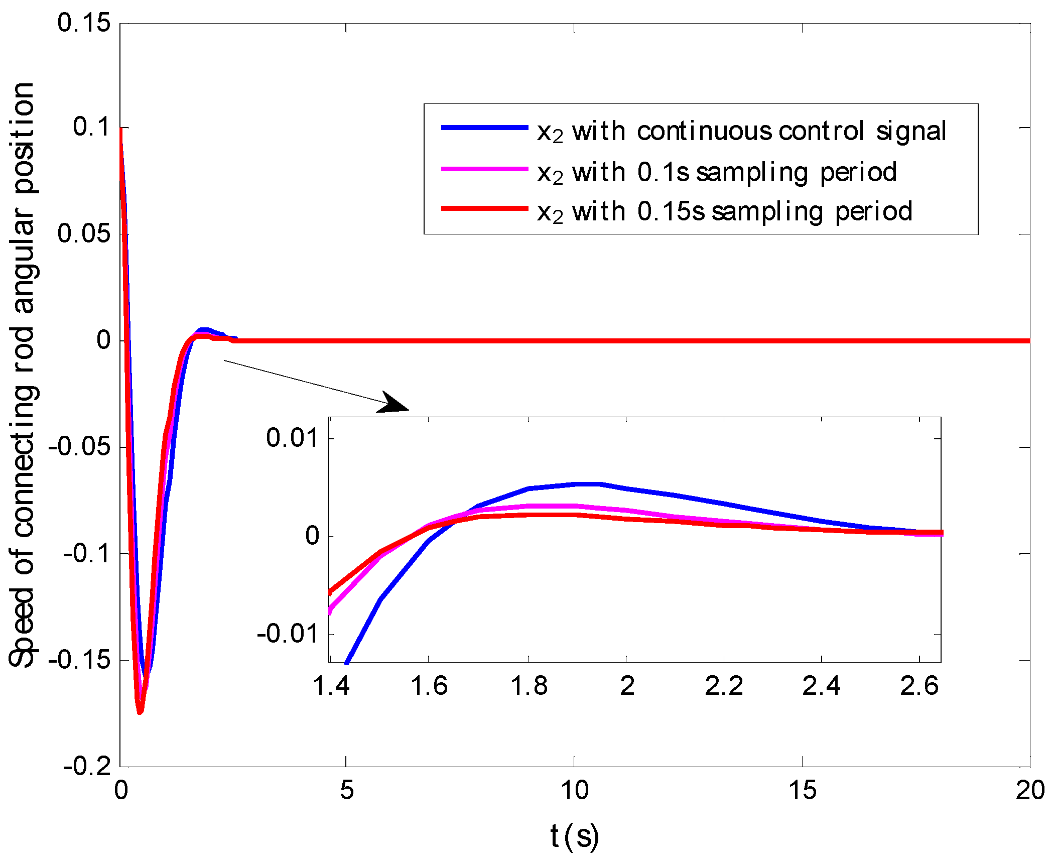
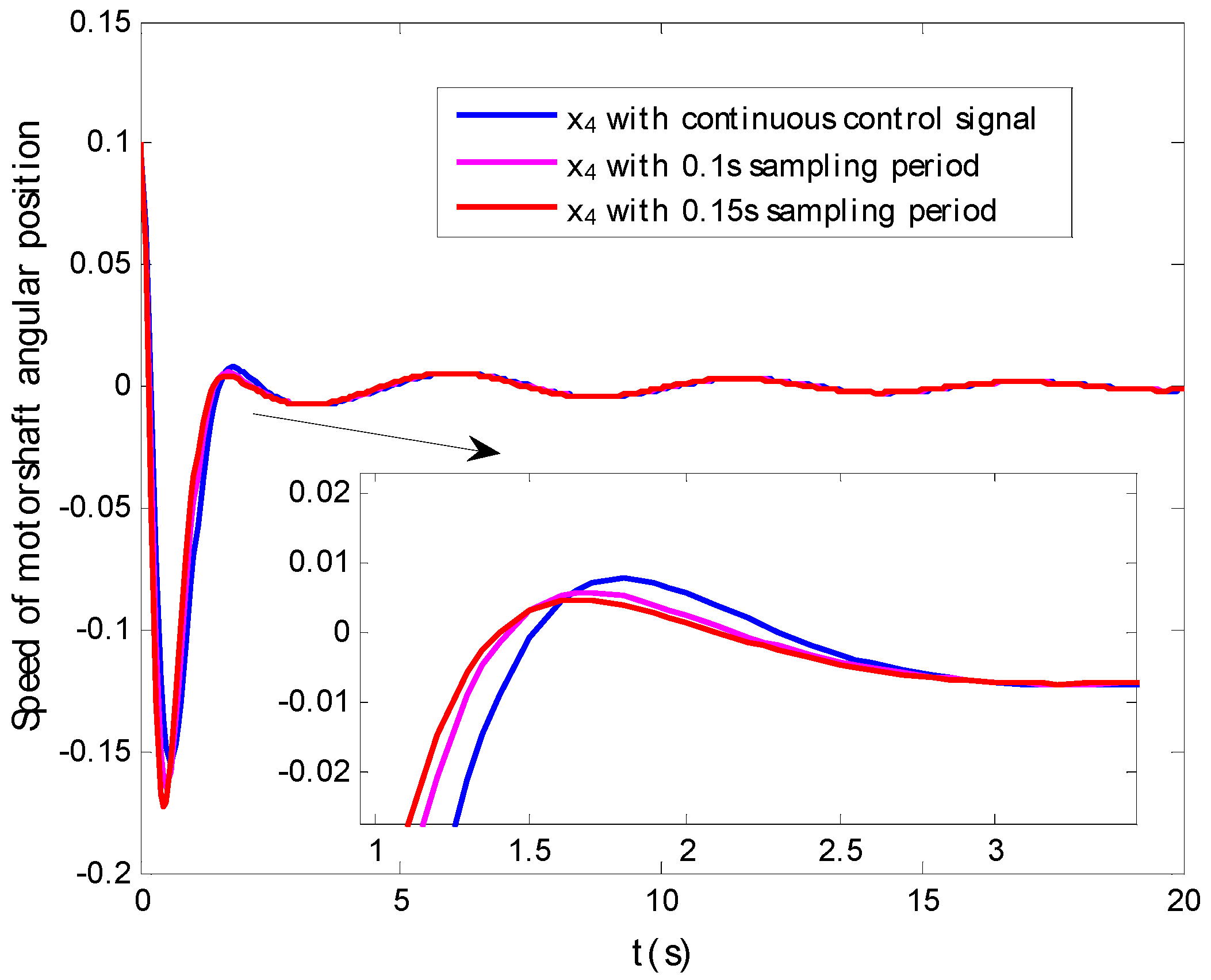
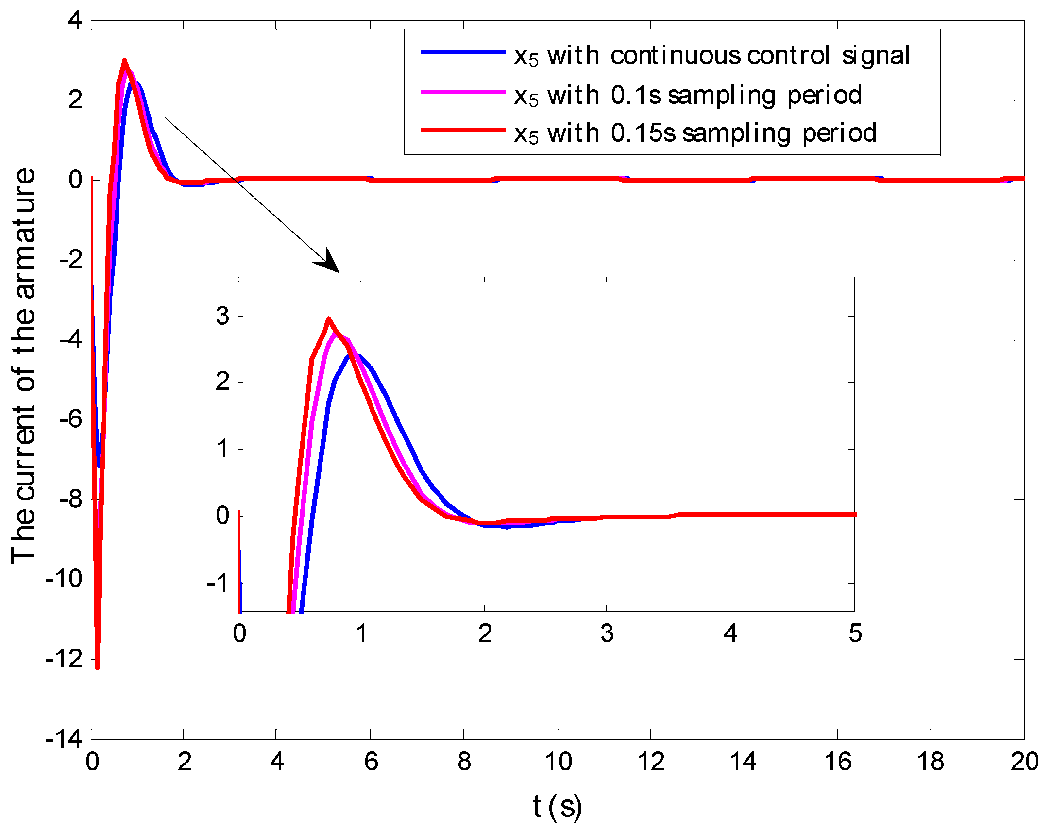
4. Simulation Results

In this section, the parameters of the flexible robotic manipulator (1) are given in Table 1.
As in Section 3, FLS is considered to address the unknown nonlinear functions. The corresponding fuzzy membership functions (see Figure 1) are chosen as
μ F 2 l ( x i ) = e [ ( x i + 3 l ) 2 4 ] ( i = 1 , 2 ) ,   μ F 3 l ( x j ) = e [ ( x j + 3 l ) 2 4 ] ( j = 1 , 2 , 3 ) μ F 3 l ( x k ) = e [ ( x k + 3 l ) 2 4 ] ( k = 1 , 2 , 3 , 4 ) ,   μ F 4 l ( x w ) = e [ ( x w + 3 l ) 2 4 ] ( w = 1 , 2 , 3 , 4 , 5 ) ( l = 1 , 2 , 3 , 4 , 5 )
The initial values of the state are chosen as x 1 ( 0 ) = x 2 ( 0 ) = x 3 ( 0 ) = x 4 ( 0 ) = x 5 ( 0 ) = 0.1 , and the initial values for other variable are set as 1. Under the proposed backstepping sampled data control method, we design the virtual control signals (8), (16), (27), and (38), the adaptive updated laws (17), (28), (39), and (50), and actual control input (49), and the related parameters are designed as c 1 = c 2 = c 3 = c 4 = 0.3 , c 5 = 1 and δ 1 = δ 2 = δ 3 = δ 4 = 5 . The fixed sampled data period is chosen as 0.2 s. The simulation results are shown in Figure 2, Figure 3, Figure 4 and Figure 5.
Form Figure 2, Figure 3, Figure 4, Figure 5, Figure 6, Figure 7 and Figure 8, we can see that the system states and the adaptive parameters converge on a small residual set. Besides, the controlled performance is further shown in Figure 2, Figure 3, Figure 4, Figure 5, Figure 6 and Figure 7 by choosing the different sampling periods and the continuous case. According to Figure 2, Figure 3, Figure 4, Figure 5 and Figure 6, we can conclude that at the inflection point of each state, the state changes faster when the sampling period is smaller. The reason for this phenomenon is that the sampled data controller is executed by the ZOH, which cannot adjust itself in time. In Figure 7, the control signals with a different sampling period and the continuous case are given. The control input signal is utilized for the controller plant in discrete form. Rather than the continuous form in [10,11,12,13,14,15,16,17,18,19,20], the designed control signal releases the constraints of the continuous state’s information.

5. Conclusions

This paper studied the backstepping sampled data control method for a flexible robotic manipulator, whose internal parameters are unknown, and FLS was employed to eliminate the uncertainties. Furthermore, in the control design, we only used the sampled data of the states to design the control signal, which means we can use less information to achieve control objective than the normal ones. By considering the SGUUB stability theory, all signals of the flexible robotic manipulator are covered within a small neighborhood of the origin. The simulation results are also given to illustrate the validity of the sampled data control algorithms. Our future research direction is output feedback sampled data control for the flexible robotic manipulator.

Author Contributions

Writing—original draft preparation, J.Z.; Writing—review and editing, X.D. All authors have read and agreed to the published version of the manuscript.

Funding

This research was funded by the Innovation Project of Guangxi University of Science and Technology Graduate Education (Grant No. GKYC202225).

Conflicts of Interest

The authors declare no conflict of interest.

References

  1. Bazzi, B.; Chalhoub, N. Fuzzy sliding mode controller for a flexible single-link robotic manipulator. J. Vib. Control 2005, 11, 295–314. [Google Scholar] [CrossRef]
  2. Ma, Z.; Sun, G. Dual terminal sliding mode control design for rigid robotic manipulator. J. Frankl. Inst. 2018, 355, 9127–9149. [Google Scholar] [CrossRef]
  3. Alam, W.; Ahmad, S.; Mehmood, A.; Iqbal, J. Robust sliding mode control for flexible joint robotic manipulator via disturbance observer. Interdiscip. Descr. Complex Syst. INDECS 2019, 17, 85–97. [Google Scholar] [CrossRef]
  4. Oliveira, J.; Oliveira, P.; Boaventura, J.; Pinho, T. Chaos-based grey wolf optimizer for higher order sliding mode position control of a robotic manipulator. Nonlinear Dyn. 2017, 90, 1353–1362. [Google Scholar] [CrossRef]
  5. Ahmed, S.; Ahmed, A.; Mansoor, I.; Junejo, F.; Saeed, A. Output feedback adaptive fractional-order super-twisting sliding mode control of robotic manipulator. Iran. J. Sci. Technol. Trans. Electr. Eng. 2021, 45, 335–347. [Google Scholar] [CrossRef]
  6. Bagheri, M.; Naseradinmousavi, P.; Krstić, M. Feedback linearization based predictor for time delay control of a high-DOF robot manipulator. Automatica 2019, 108, 108485–108492. [Google Scholar] [CrossRef]
  7. Korayem, M.; Nekoo, S.; Kazemi, S. Finite-time feedback linearization (FTFL) controller considering optimal gains on mobile mechanical manipulators. J. Intell. Robot. Syst. 2019, 94, 727–744. [Google Scholar] [CrossRef]
  8. Belherazem, A.; Chenafa, M. Passivity based adaptive control of a single-link flexible manipulator. Autom. Control Comput. Sci. 2021, 55, 1–14. [Google Scholar] [CrossRef]
  9. Feliu, D.; Feliu, V. Passivity-based control of a single-link flexible manipulator using fractional controllers. Nonlinear Dyn. 2019, 95, 2415–2441. [Google Scholar] [CrossRef]
  10. Keighobadi, J.; Fateh, M.; Xu, B. Adaptive fuzzy voltage-based backstepping tracking control for uncertain robotic manipulators subject to partial state constraints and input delay. Nonlinear Dyn. 2020, 100, 2609–2634. [Google Scholar] [CrossRef]
  11. Sun, W.; Su, S.; Xia, J.; Nguyen, V. Adaptive fuzzy tracking control of flexible-joint robots with full-state constraints. IEEE Trans. Syst. Man Cybern. Syst. 2018, 49, 2201–2209. [Google Scholar] [CrossRef]
  12. Zhang, C.; Yang, T.; Sun, N.; Fang, Y. An adaptive fuzzy control method of single-link flexible manipulators with input dead-zones. Int. J. Fuzzy Syst. 2020, 22, 2521–2533. [Google Scholar] [CrossRef]
  13. Ling, S.; Wang, H.; Liu, P. Adaptive fuzzy dynamic surface control of flexible-joint robot systems with input saturation. IEEE/CAA J. Autom. Sin. 2019, 6, 97–107. [Google Scholar] [CrossRef]
  14. Fateh, S.; Fateh, M. Adaptive fuzzy control of robot manipulators with asymptotic tracking performance. J. Control Autom. Electr. Syst. 2020, 31, 52–61. [Google Scholar] [CrossRef]
  15. Wang, Z.; Zou, L.; Su, X.; Luo, G.; Li, R.; Huang, Y. Hybrid force/position control in workspace of robotic manipulator in uncertain environments based on adaptive fuzzy control. Robot. Auton. Syst. 2021, 145, 103870–103881. [Google Scholar] [CrossRef]
  16. Diao, S.; Sun, W.; Yuan, W. Adaptive fuzzy practical tracking control for flexible-joint robots via command filter design. Meas. Control. 2020, 53, 814–823. [Google Scholar] [CrossRef]
  17. Datouo, R.; Ahanda, J.; Melingui, A.; Biya-Motto, F.; Zobo, B. Adaptive fuzzy finite-time command-filtered backstepping control of flexible-joint robots. Robotica 2021, 39, 1081–1100. [Google Scholar] [CrossRef]
  18. Li, Y.; Tong, S.; Li, T. Adaptive fuzzy output feedback control for a single-link flexible robot manipulator driven DC motor via backstepping. Nonlinear Anal. Real World Appl. 2013, 14, 483–494. [Google Scholar] [CrossRef]
  19. Chang, W.; Li, Y.; Tong, S. Adaptive fuzzy backstepping tracking control for flexible robotic manipulator. IEEE/CAA J. Autom. Sin. 2021, 8, 1923–1930. [Google Scholar] [CrossRef] [Green Version]
  20. Khorashadizadeh, S.; Sadeghijaleh, M. Adaptive fuzzy tracking control of robot manipulators actuated by permanent magnet synchronous motors. Comput. Electr. Eng. 2018, 72, 100–111. [Google Scholar] [CrossRef]
  21. Li, S.; Ahn, C.; Guo, J.; Xiang, Z. Neural network-based sampled-data control for switched uncertain nonlinear systems. IEEE Trans. Syst. Man Cybern. Syst. 2019, 51, 5437–5445. [Google Scholar] [CrossRef]
  22. Li, S.; Ahn, C.; Xiang, Z. Sampled-data adaptive output feedback fuzzy stabilization for switched nonlinear systems with asynchronous switching. IEEE Trans. Fuzzy Syst. 2018, 27, 200–205. [Google Scholar] [CrossRef]
  23. Davó, M.; Bresch-Pietri, D.; Prieur, C.; Meglio, F. Stability analysis of a 2 × 2 linear hyperbolic system with a sampled-data controller via backstepping method and looped-functionals. IEEE Trans. Autom. Control. 2018, 64, 1718–1725. [Google Scholar] [CrossRef]
  24. He, W.; Ahn, C.; Xiang, Z. Global fault-tolerant sampled-data control for large-scale switched time-delay nonlinear systems. IEEE Syst. J. 2019, 14, 1549–1557. [Google Scholar] [CrossRef]
  25. Mao, J.; Guo, J.; Xiang, Z. Sampled-data control of a class of uncertain switched nonlinear systems in nonstrict-feedback form. Int. J. Robust Nonlinear Control 2018, 28, 918–939. [Google Scholar] [CrossRef]
  26. Li, Y.; Yu, K. Adaptive fuzzy decentralized sampled-data control for large-scale nonlinear systems. IEEE Trans. Fuzzy Syst. 2021, 30, 1809–1822. [Google Scholar] [CrossRef]
Figure 1. The fuzzy rules.
Electronics 11 02270 g001
Figure 2. The trajectories of state x1 with different sampling periods.
Electronics 11 02270 g002
Figure 3. The trajectories of state x 2 with different sampling periods.
Electronics 11 02270 g003
Figure 4. The trajectories of state x 3 with different sampling periods.
Electronics 11 02270 g004
Figure 5. The trajectories of state x 4 with different sampling periods.
Electronics 11 02270 g005
Figure 6. The trajectories of state x 5 with different sampling periods.
Electronics 11 02270 g006
Figure 7. The trajectories of sampled control signal u with different sampling periods.
Electronics 11 02270 g007
Figure 8. The trajectories of adaptive parameters θ ^ i ( i = 1 , 2 , 3 , 4 ) .
Electronics 11 02270 g008
Table 1. The parameters of flexible robotic manipulator.
SymbolValueUnitSymbolValueUnit
F 1 3Nms/rad F 2 3Nms/rad
J 1 30kg·m2 J 2 30kgm2
R 10 Ω K a 3Nm/A
L 6H K t 0.976Nm/A
d 0.4m m 0.102kg
g 9.8N/kg K 20\
N 1\
Publisher’s Note: MDPI stays neutral with regard to jurisdictional claims in published maps and institutional affiliations.

