1. Introduction
The concept of digital twins is relatively fresh [
1,
2]. It takes and mixes known modeling and simulation techniques, giving practitioners new opportunities and tools for system development and analysis [
3,
4,
5]. New approaches to data combined with their digital representation of a real system, that may exist or not, create new perspectives, enhancing design, necessary maintenance repeated every day and future improvements [
6]. The digital twins approach requires the formulation of a virtual replica of the considered process.
Methodological assumptions behind the digital twins concept are straightforward. A digital twin of the process is developed. The digital twin offers the possibility of carrying out essential development steps, i.e., design of a control system structure, verification of our assumptions concerned with process operation and initial validation of the system use. We accept that the accuracy of the digital twin is limited and our hypothesis will be validated when the real system is available. However, the application of the digital twins concept demands specific knowledge from many research contexts: data analysis, machine learning, simulation and modeling accompanied by the specific knowledge about the target real process technology [
7,
8]. Process operators may benefit from training using a digital twin platform. Furthermore, a digital twin can also be utilized to investigate cybersecurity problems and suggest necessary protection measures [
8,
9].
A digital twin application addressed in the current research considers the high energy detector utilized in high energy physics experiments to detect elementary particles. New installations are now under construction in a few research centers.
The described digital twin research focuses on the Thermal System (TS) and its thermal protection cooling system. The Silicon Tracking Detector (STD) consists of cylindrical layers that are coaxial with the beam pipe. The STD performs reconstruction of primary and secondary vertices. Moreover, it improves the tracking abilities close to the interaction point. An excellent review article on STDc is [
10], different technological issues and examples of utilization are given in [
11,
12,
13]. Its thermal system has to maintain proper conditions (pressure and temperature) of a cooling liquid at all crucial points of the detector. The digital twin replicates it. As the full-scale STD detector is under construction, it requires initial validation and it has to be equipped with an efficiently working control system.
The above assumption opens the door for the introduction of the digital twin. Previously used methodology assumed that the system customization, control system design and its tuning could only be conducted once the process already exists. The digital twin of the new installation under design allows to speed up the whole implementation process. Many issues may be solved earlier and various alternatives validated before the installation is commissioned, which excludes further implementation time losses. This fact is particularly important and helpful for the control system design. This issue is part of the traditional methodology of implementing an industrial control system; when installation and tuning on a real facility SAT (Site Acceptance Test) is always preceded by FAT (Factory Acceptance Test). The digital twin is a rational alternative that addresses this issue.
Let us formulate the goal of this research. This work presents a general methodology to design a control system structure for a TS using the digital twin approach. The considered TS is an example process; this work does not attempt to develop a complete control system for a particular TS. The digital twin of the TS is developed using Simscape simulation technology for a not existing yet full-scale target system. Its operation is validated against technology constraints and process goals. The digital twin-based system is supplied with a specifically designed control system, assuring cooling temperature operating regimes. The TS digital replica is used to select the appropriate control philosophy and develop the control system structure that will be implemented within the target control system hardware when it is available. It must be stressed that this digital twin-based work aims to develop a general control system structure and very rough tuning of the controllers’ parameters. Precise tuning will be carried out when the real process is available. It is a typical approach; we never rely on controllers tuned using only mathematical models, tuning taking into account the real process behavior is always necessary. Moreover, we expect that the values of the model parameters used in simulations presented in this work may differ from real parameters.
This article is structured as follows. At first,
Section 2 describes the high energy physics setup, including multi-detector experiments, scientific aims of the STD, the general layout of STDs.
Section 3 presents the design procedure and structure of the developed thermal system. Next,
Section 4 introduces possible simulations technologies. The main part of this article is given in
Section 5, which details the completed digital twin application for the STD cooling system.
Section 6 demonstrates model validation and simulation results. Finally,
Section 7 summarizes the whole article.
2. High Energy Physics Setup
2.1. Multi-Detector Experiments
For many years, physicists worldwide have been looking for answers to questions posed by the constantly developing field of quantum physics. In order to find the answers to at least some of them, various types of high-energy physics experiments are carried out at research centers such as CERN, Brookhaven National Laboratory, GSI Helmholtz Center for Heavy Ion Research, and Joint Institute for Nuclear Research. The experiments investigating ion collisions are particularly promising and popular, but they require massive infrastructure and engineering facilities. Two subgroups can be distinguished among this type of experiment, i.e., fixed target and experiments on colliders. In the first one, packets of ions, previously accelerated with an acceleration chain, are directed to a stationary target. Examples of such experiments are CBM (Compressed Baryonic Matter) [
14], HADES (High Acceptance Di-Electron Spectrometer) [
15], and BM@N (Baryonic Matter at Nuclotron) [
16]. In the second type of experiments, two beams accelerated in opposite directions are collided at interaction points. In this case, one can distinguish, among others, STAR (Solenoidal Tracker at RHIC) [
17], ALICE (A Large Ion Collider Experiment) [
18], CMS (Compact Muon Solenoid) [
19], ATLAS (A Toroidal LHC ApparatuS) [
20], MPD (Multi-Purpose Detector) [
21] experiments. In both cases, in the areas of ion collisions, groups of scientists set up an experimental set-up made of multiple detectors.
Despite some differences in the structure of the multi-detectors mentioned above, the purpose of their operation is similar, i.e., the identification of particles with parameters specified for the experiment and their kinematics. Depending on the experiment, various detectors may be used to achieve this goal, e.g., trackers, calorimeters, time-of-flight detectors. On the other hand, the common feature of all of these experiments is the use of strong magnets that create a constant magnetic field and bend the trajectory of the long-lived charged particles created as a result of the collision. Information about these particles’ charge and momentum is obtained by measuring their trajectory’s curvature. To measure this, the STDs are widely used.
2.2. Scientific Aims of Silicon Tracking Detectors
One of the leading physics aims of the multi-detectors is to study the properties of hot and dense nuclear matter produced in collisions of heavy nuclei at various energy ranges [
18]. There are a considerable number of different particles which may be created after the ion collisions [
18]. The lightest hadrons, such as pions or kaons, have a relatively long lifetime, so they may be registered and studied by the detectors located relatively far from the point of interaction [
22]. By the theoretical predictions, heavy quarks (c—charm, b—beauty) are born in the initial state of the heavy nuclei collisions and carry information about the early stage of its formation [
23]. Due to that, particles made of those quarks are considered as the sources of information about the properties of strongly interacting matter [
24]. To identify and reconstruct the kinematics of such short-lived particles (multistrange hyperons, charmed mesons, hypernuclei), multi-detectors are equipped with vertex detectors located as close to the collision point as possible.
STDs are usually multilayer systems of position-sensitive sensors which have a pivotal role in improving the accuracy of the secondary decay vertices coordinates and particles with small transverse momentum reconstruction [
25].
2.3. General Layout of the Silicon Tracking Detectors
Silicon tracking detectors in experiments at colliders are located around the interaction point. Usually, the modules of the detector create a cylinder whose axis of rotation is situated on the beam, with sensor modules arranged in several layers. Moreover, modules could be overlapped to provide complete coverage of the azimuth angle. This kind of detector often is constructed in stages. The general layout of this type of silicone tracking detector is shown in
Figure 1.
Silicon tracking systems in the experiments with the fixed target are located behind the target. Usually, the whole detector is mounted inside a dipole magnet. The detector contains a few layers of the modules located perpendicularly to the beam axis. The general layout of this type of silicone tracking detector is shown in
Figure 2.
Nowadays, the most popular sensors used in silicon tracking detectors are monolithic Active Pixel Sensors (MAPS). The typical sizes of such a sensor are between 15 × 30 [mm
] [
25] and 62 × 62 [mm
] [
13]. A single module of the detector contains the matrix of MAPS sensors. For example, outer layer modules of the ALICE-ITS (in experiments at colliders) have a length of 1500 mm and are wide of 60 mm. The outer radius of this detector is around 450 mm [
26].
Since silicon tracing detectors are typically placed in the center of the experimental set-up, low material budget and low heat emission are required. The problem of the material budget is mainly solved by mounting detection modules on lightweight mechanical support ladders. Moreover, those ladders are made using materials with low nuclear cross-section, such as carbon fiber composite. Further, this article describes one approach to solving the heat emission problem.
The temperature stabilization for the STD system is crucial to maintain the high detection performance of the detector. Its cooling system consists of two subsystems: air and liquid cooling. Liquid cooling maintains the proper temperature in the staves with cooling panels using feed/return lines. Air cooling uses air nozzles located around the staves. The main objectives of the thermal system control are to maintain at a given level the following variables:
Very low temperature gradient on the detector;
Very low heat transfer from STD to other detectors;
Temperature gradient inside the detector volume not bigger than 0.5 C;
Constant air flow through detector;
Absence of vibration that may be caused by air flow bigger than 2 m/s;
Required humidity of the air inside the detector.
The simplified Piping and Instrumentation diagram (P&ID) diagram presenting the liquid cooling system for three staves is shown in
Figure 3. It consists of the cooling liquid tank reservoir (BB501), the pumps (AP401 and AP601), chiller (AH101) and several flow (CF), pressure (CP) and temperature (CT) sensors. The simplified system makes it possible to verify technological assumptions, particularly those concerned with the control system and performance assessment.
3. Thermal System: Design Procedure and Structure
The system design procedure is presented in
Figure 4. This is a multi-stage process to achieve a fully functioning system. It is crucial to underline that during the whole design process, the risk of error or damage to the actual object is eliminated. All tests and modifications are undertaken at the design and verification stage on the simulator, which allows the detection and elimination of irregularities before the phase of implementation on the real object.
In the first step, a functional design is made, describing the considered system’s intended capabilities, design, and user interactions. A functional specification must be formulated. Its role is to characterize the system’s required properties and behavior. Additionally, all details related to interactions with users, as well as descriptions for engineers who next implement the system and software developers.
Based on the functional specification, the technical design is created in the second step of the process. It gives all necessary implementation details of the system so that it fulfils all of the functions assigned to it. The technical design provides detailed information about how the product will be built. It describes the technology, software, hardware and capabilities. The description of how data will be collected, exchanged and stored is necessary. Because of the technical nature of this document, it must be written by a technical person, i.e., someone who understands the hardware and software constraints and capabilities and can communicate the requirements to the developer.
In the next step, controls and the process model are made in MATLAB, based on the technical specification. The idea is to allow running a simulation of the system in MATLAB using a proper control strategy. Control system outputs are updated during the simulation. At this stage, it is possible to eliminate conceptual errors in the control structure and to check the properties of the control structure, such as robustness, accuracy and response dynamics.
After the system has been validated in MATLAB, the real control system is implemented on the Programmable Logic Controller (PLC). A connection is established between MATLAB and the PLC and the Supervisory Control And Data Acquisition (SCADA) system. The SCADA system is used to visualize the control system and allow user interaction with the system. At this stage, the operation of hardware and software is checked. Data flow and addressing are verified. The Human Machine Interface (HMI) functionality and the required functions are checked, particularly the ability to control the process fully. Data acquisition systems are configured and control quality analysis is carried out.
The final stage of the procedure is to verify the control system by controlling the actual thermal process with a control system implemented on a PLC. In short, a real process is used in place of the digital twin-based simulator. This is a multi-part stage. The first sub-step is to check the cable addressing whether the object has been correctly connected and whether it is possible to influence all the actuators. Next, cold tests are carried out, i.e., the possibility of influencing individual sections of the process. These tests are carried out on a not-yet-started process. Positive results from the individual sections allow for the gradual start-up of the process and the execution of tests on a fully operational plant. It is important to stress that even in simulations, the control system is implemented using a real industrial PLC; similarly, a real industrial SCADA system is used for process monitoring and visualization. It means that these components are the same in simulations and when a real process replaces the simulator.
4. Simulation Technologies
The simulated process model has a specific structure. It is presented in the form of a diagram in
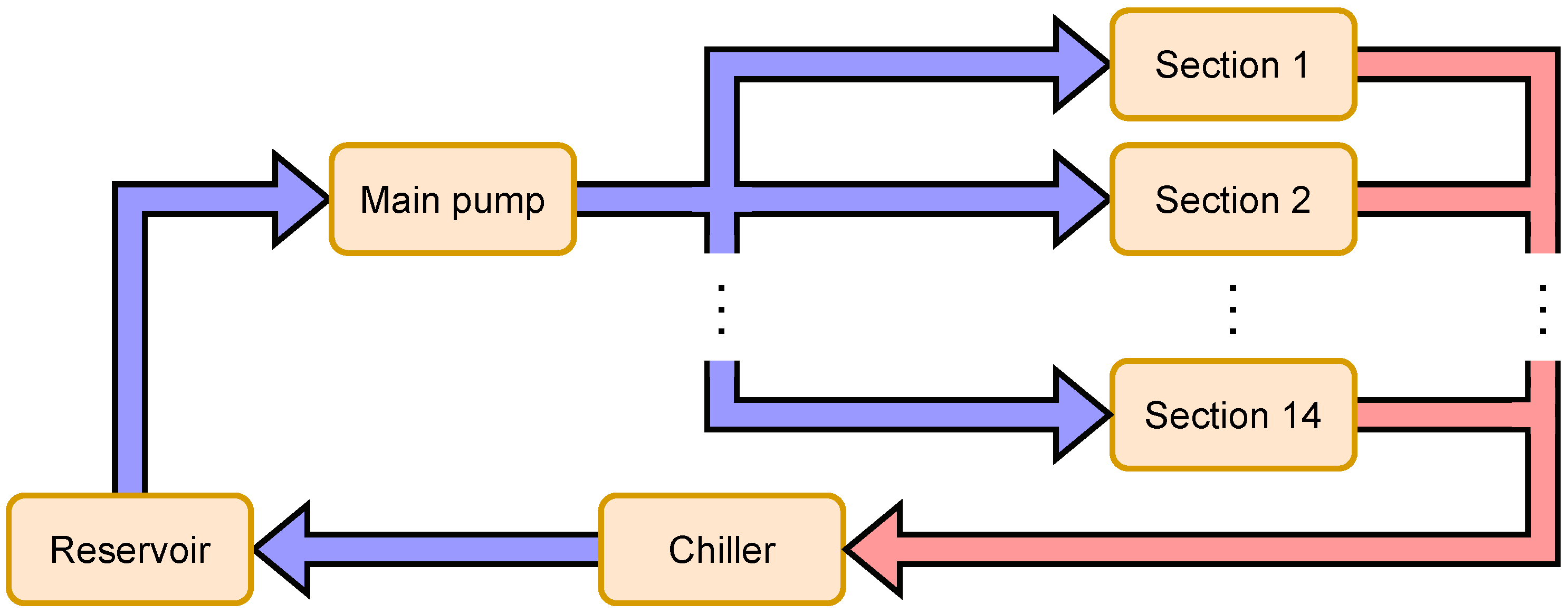
Figure 5. There is a Reservoir block, in which a vacuum system is implemented that provides leak-less technology conditions in conjunction with the liquid domain. The Main pump block mainly consists of the pump, which gives the liquid flow through the detector. There are 14 sections in total. The input of each section block is the liquid with a lower temperature and the output is the liquid with a higher temperature. The liquid gets heated up whenever it passes through a section. It is then chilled after passing the Chiller block.
The process simulation has been realized in the MATLAB environment supported by the Simulink package. In particular, the Simscape library has beenused. This choice has been motivated by the fact that Simscape allows the dynamic states of the process to be simulated easily and, at the same time, gives great flexibility to the programmer. Examples of the use of the library can be found, among others, in systems where it is used to model variable pressure, flow, and temperature of liquids and gases [
27]. It is also used in electrical and mechanical systems [
28,
29].
Smiscape allows liquids and gases to be easily defined through several parameters. The system is built through prefabricated building blocks such as valves, pipes, and flow controllers. This approach allows the system to be intuitively reproduced directly from the P&ID diagram. As a result, any Thermal System changes can be easily reproduced in the simulated environment. On the other hand, the simulation can serve as a place to test changes before possibly incorporating them into the real system.
In the Simulink package, it is possible to define a series of differential equations that describe the relationships between signals in the system. In the case of the Thermal System, only some of this functionality has been used. The focus has been on modeling only the gas and liquid flowing through the system. Therefore, only relevant values such as pressures, temperatures, mass and volume flows are measured. It should be noted that Simscape also allows phenomena such as thermal convection between different system components to be modeled.
The input signals to the designed, simulated system are the control signals generated by the controllers implemented in the PLC. The outputs, on the other hand, are measurements of simulated temperatures, pressures, and flows. As a result, the simulated part of the system is enclosed in a single block, which can be easily replaced by real equipment if required. Simulation tests can be carried out without any changes to the hardware. Only when the system changes have been tested and verified in the simulation can analogous changes be made to the physical system, thus completing the implementation process.
An OPC UA server has been used for communication between the simulated system and the PLC. It is a standard tool used in this type of application, enabling data transmission between MATLAB and the PLC.
5. Digital Twin Application for Thermal System
5.1. Simscape Process Model
Simscape offers a broad range of elements that can be used to create simulated thermal systems, including reservoirs, various sources, pipes and measuring equipment, e.g., pressure and temperature sensors, mass and energy flow rate sensors or volumetric flow rate sensors [
30]. It also allows for real-time simulation, which is a key feature for future SCADA and control structures testing [
31]. Simscape Thermal Liquid library offers blocks that enable the use of thermal effects in a fluid process simulator. Various blocks are available, e.g., basic elements, sensors and sources. Using the above elements, the simulated process has been developed. Simulation has been performed for signal change scenario and results presented.
5.2. Control and SCADA System
The system is intended to be controlled in two loops:
- Loop 1:
The pressure regulator controls the pressure value at the inlet to each section. The value must not be higher than atmospheric pressure.
- Loop 2:
The flow controller keeps the flow at such a level that the temperature in any section at any half stave does not exceed 22 C. The controller impacts the flow by the valve.
The system in this “primitive” assumes that the facility is symmetrical and the coolant distribution is uniform. Both assumptions are not true in reality; it is natural for higher temperatures to occur in the higher sections (the unit will be mounted horizontally). A second reason for the asymmetry may be that some section needs to be shut down. The assumption of a uniform flow may also not be met in practice due to the different lengths and shapes of the tubes.
Considering the above, it is suggested to install valves at the input of each section, which would allow the throttling of sections where the output temperatures from the half stave are the lowest so that the final temperature is as equal as possible in all sections. In addition, such valves would allow any section to be shut off in case of a leak (but valves on the output would still be necessary).
The structures sketched in
Figure 6,
Figure 7,
Figure 8 and
Figure 9 are subject for future investigation (these figures have been generated using an industrial SCADA system and show a really implemented control systems). All control loops are treated as independent in the basic structure shown in
Figure 6. The suction pump controls the pressure; the temperature is controlled by cascaded Proportional-Integral-Derivative (PID) algorithms, where the lower PID affects the position of the pump valve and controls the liquid flow. The heater is responsible for the temperature. The temperature in each section is controlled by a single PID algorithm, which affects the position of the suction valve.
The heater is controlled by a single PID and feed-forward module in the base structure extended about feed forward shown in
Figure 7. This structure is proactive, using a gas flow that directly affects the heater.
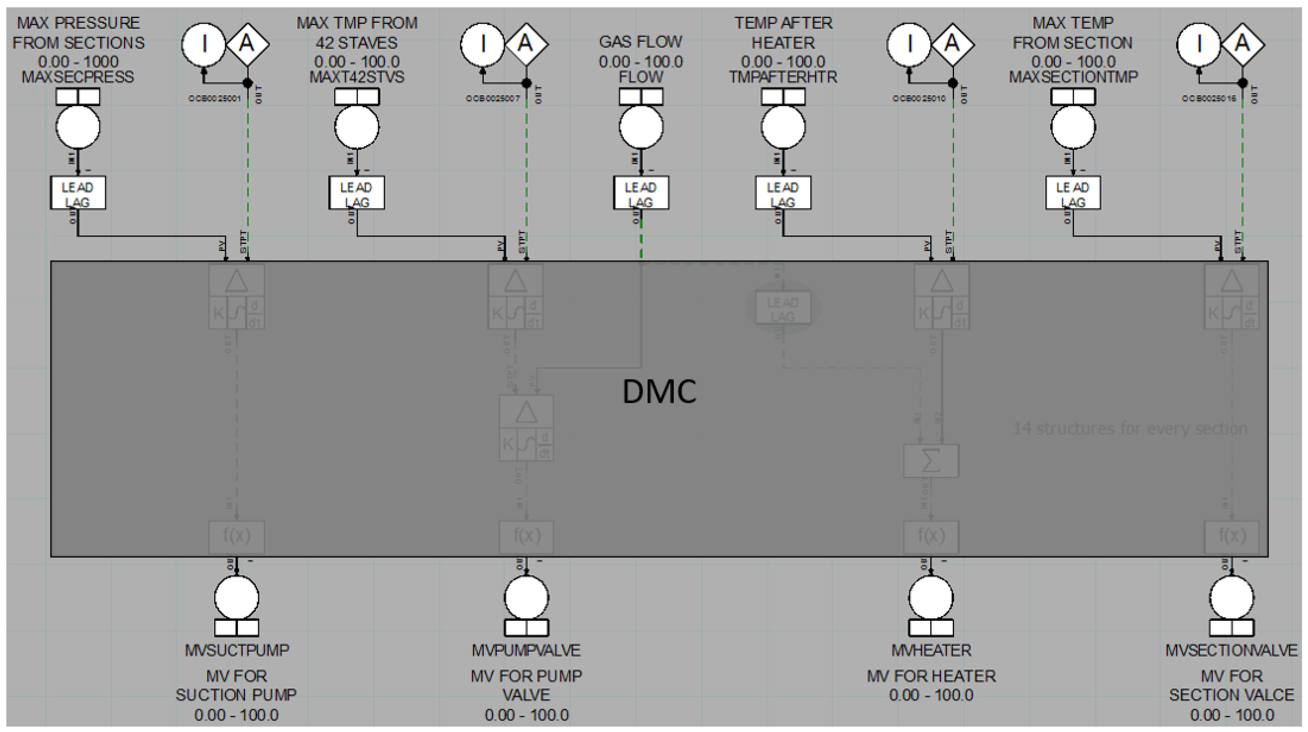
The two control loops responsible for the pump and heater valve and the feed-forward module can be replaced by a multivariable Dynamic Matrix Control (DMC) algorithm. Due to the process’s stable nature, the DMC (Dynamic Matrix Controller) controller will be used, combining the model’s simplicity with high robustness to process disturbances. The structure in the advanced version is shown in
Figure 8.
The structure in the advanced version can be extended to the full version, where all loops are replaced by a single multivariable DMC algorithm, as shown in
Figure 9. This approach allows any interactions between the different control loops to be considered.
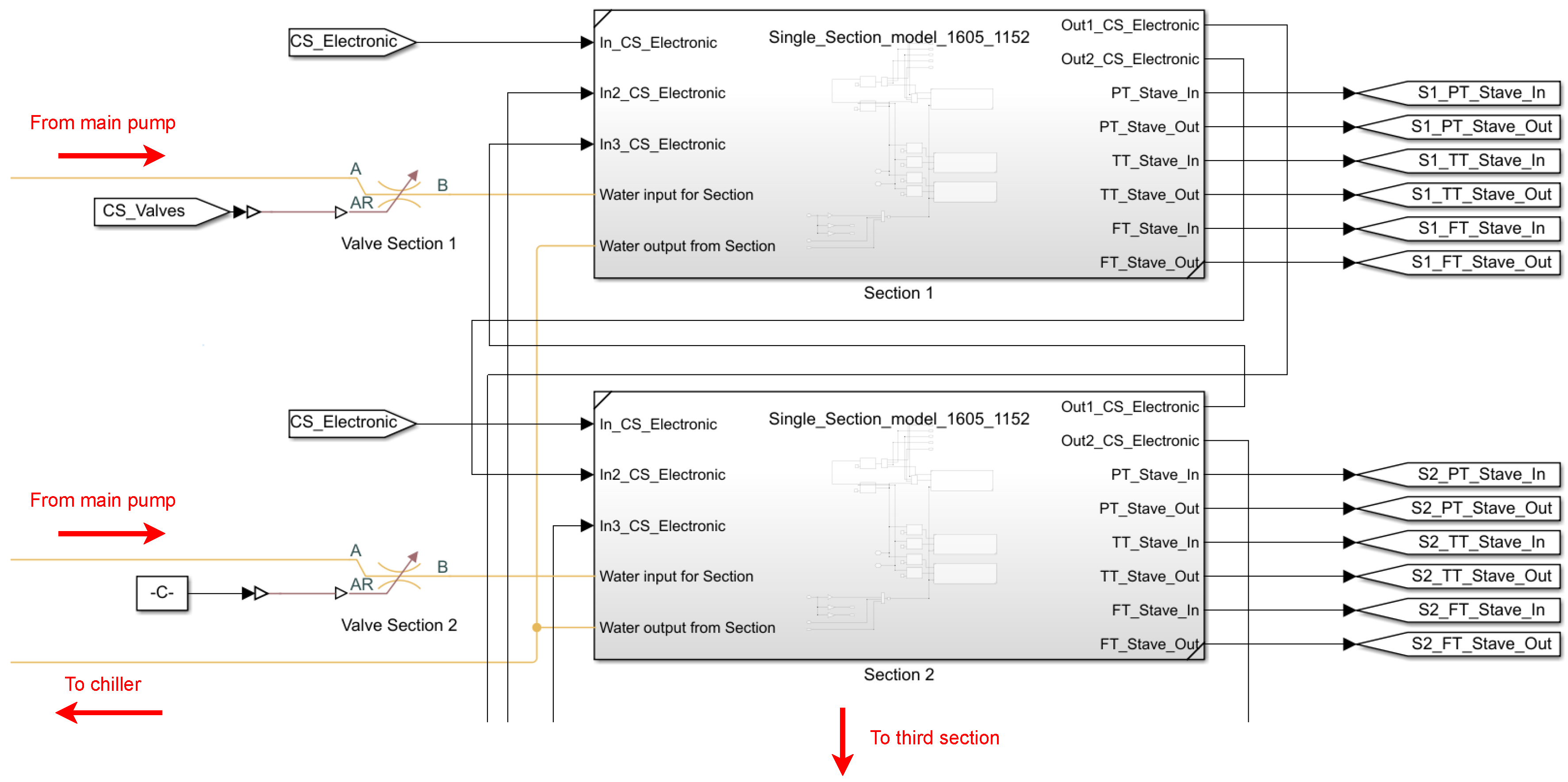
The whole process consists of the following sub-elements: chiller installation, main pump, reservoir with leak less under pressure, single stave unit, and the section containing three staves.
Figure 10,
Figure 11,
Figure 12,
Figure 13,
Figure 14,
Figure 15,
Figure 16,
Figure 17 and
Figure 18 present a detailed look at the fragments of the simulated part of the whole system
Figure 5. The simulation takes control signals from PLC controllers as inputs via the OPC UA server. At the same time, it sends the measurements of simulated variables to the PLC.
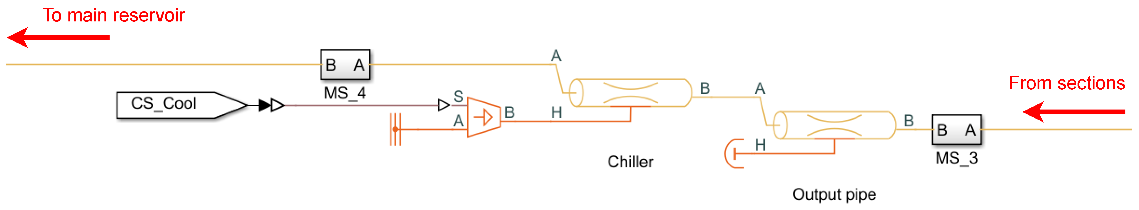
Figure 10 shows the chiller section, where the return pipe from the detector is connected to the measurement unit. Next, we can observe a pipe with a thermal element that can add or remove heat from the liquid going through. A measurement unit measures the output temperature and simple PID control is performed to achieve stable liquid temperature transferred to the reservoir.
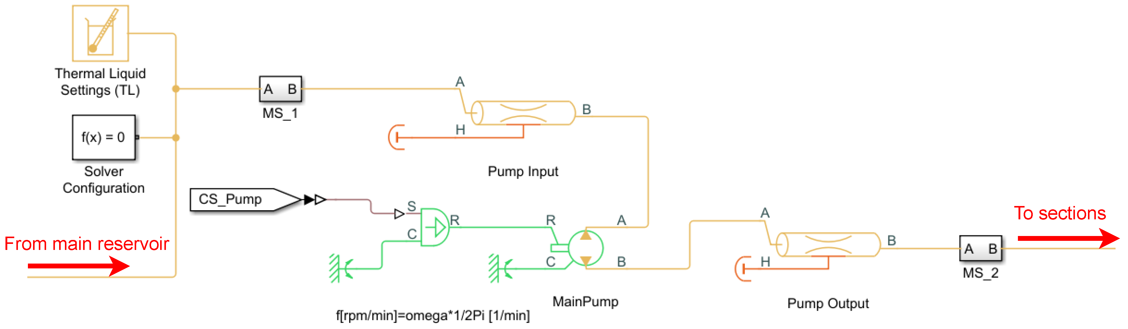
Figure 11 shows the main pump, which gives the liquid flow through the detector. The actuating element is a pump with adjustable flow, which is now constant and dependent on the number of detector sections. Measurements are possible before and after the pump.
Figure 12 shows a vacuum system’s component that provides leak-less technology conditions in conjunction with the liquid domain. Underpressure can be adjusted by an ideal pressure pump in the gas domain. Thanks to the used reservoir, both gas and liquid domains are mixed and finally, we achieve the leak-less simulation process.
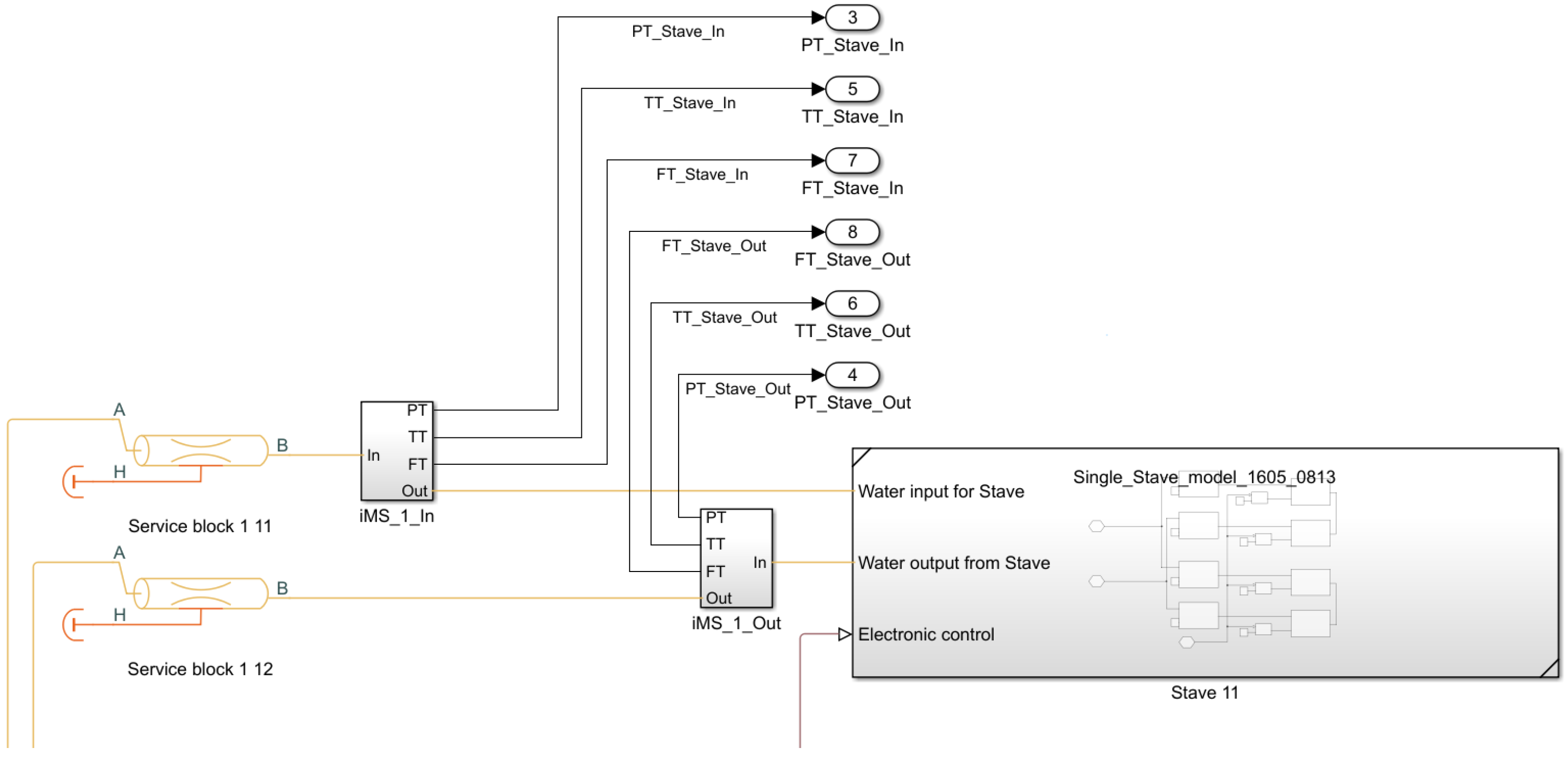
Figure 13 shows the internal structure of a single stave, which is a part of a section in the detector unit. We can observe liquid main input and output. The third connection is for the simulation of electronics which delivers heat to the liquid.
Figure 14 shows two staves connected to the liquid network using a subsystem block. This schematic can make it easier to understand and locate the main parts. An additional valve is added to the first stave to test further control possibilities.
In addition to using dedicated blocks for heat transfer, a simpler approach simulates the interaction between sections.
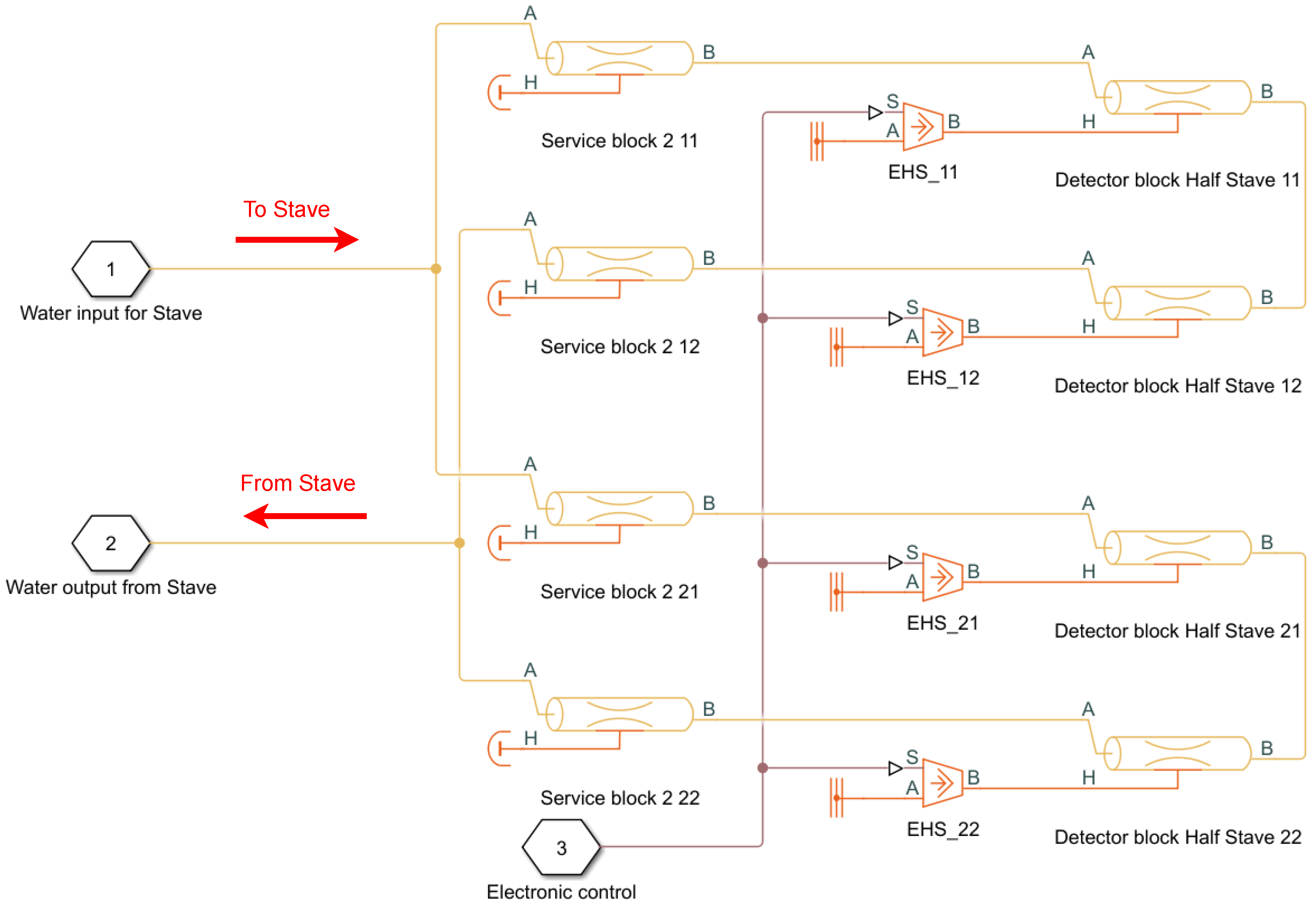
Figure 15 shows the connections between two adjacent sections. The primary connections are, of course, the coolant input and output with an additional proportional valve to make it possible to symmetrize the entire cylindrical block. Each section has an electronics control input that controls the level of heat released by the simulated electronics layer. In addition, input signals from adjacent sections combine with the main control signal to provide coupling between sections and the main control.
Figure 16 shows the details of the internal structure of a single section, where the transfer of signals from adjacent sections and also the main signal controlling the electronics is clearly shown. After consulting with experts, they confirmed that the coolant circulation receives half of the heat generated in the section. In contrast, the other half passes through convection to the air and affects the neighboring sections. This is simulated by directly splitting the electronics control signal into the main 50 percent heat control in a section and two signals going out to adjacent sections of 25 percent each. Finally, the input signals from the adjacent section signals are added to the main control signal.
Figure 17 shows the details of the internal structure of a single section, where the measure part is exposed. The three most important parameters, i.e., temperature, flow and pressure, are measured at the input and output.
Figure 18 shows an alternative approach used to simulate single stave. The stave is divided into three sections: valves with temperature, pressure and flow sensors, piping, and detector half stave blocks.
6. Model Validation and Simulation Results
Key features of the simulation are:
Liquid circulates in a closed loop;
The vacuum pump in the tank;
Forced circulation by the pump;
The number of sections to be selected depending on the calculation unit (min. 1 max. 14);
Cooling of the heated water through a heat transfer pipe;
Cold water circulation to the exchanger;
Thermal coupling between staves and sections.
The simulation scenario is:
T = 100 s start-up of the vacuum pump in the gas domain: atmosphere suction;
T = 500 s opening of input valves of all sections;
T = 700 s starting of the pump of fluid circulation at the value of flow corresponding to one section (3 staves);
T = 1200 s start of the electronics, i.e., heat is supplied to the stave;
T = 1500 s closing the valve of
Section 2. It shows the system’s desymmetrization and the interaction between sections—the temperature in
Section 1 and
Section 3 increases.
Concerning the above simulation scenario, appropriate blocks have been prepared to generate control signals. Unit jumps and first-order inertia have been used to soften the slopes of the signals before delivering them to control elements such as heaters or pumps.
Figure 19 shows a section of the signal generation blocks.
The pressure change during simulation is shown in
Figure 20,
Figure 21,
Figure 22 and
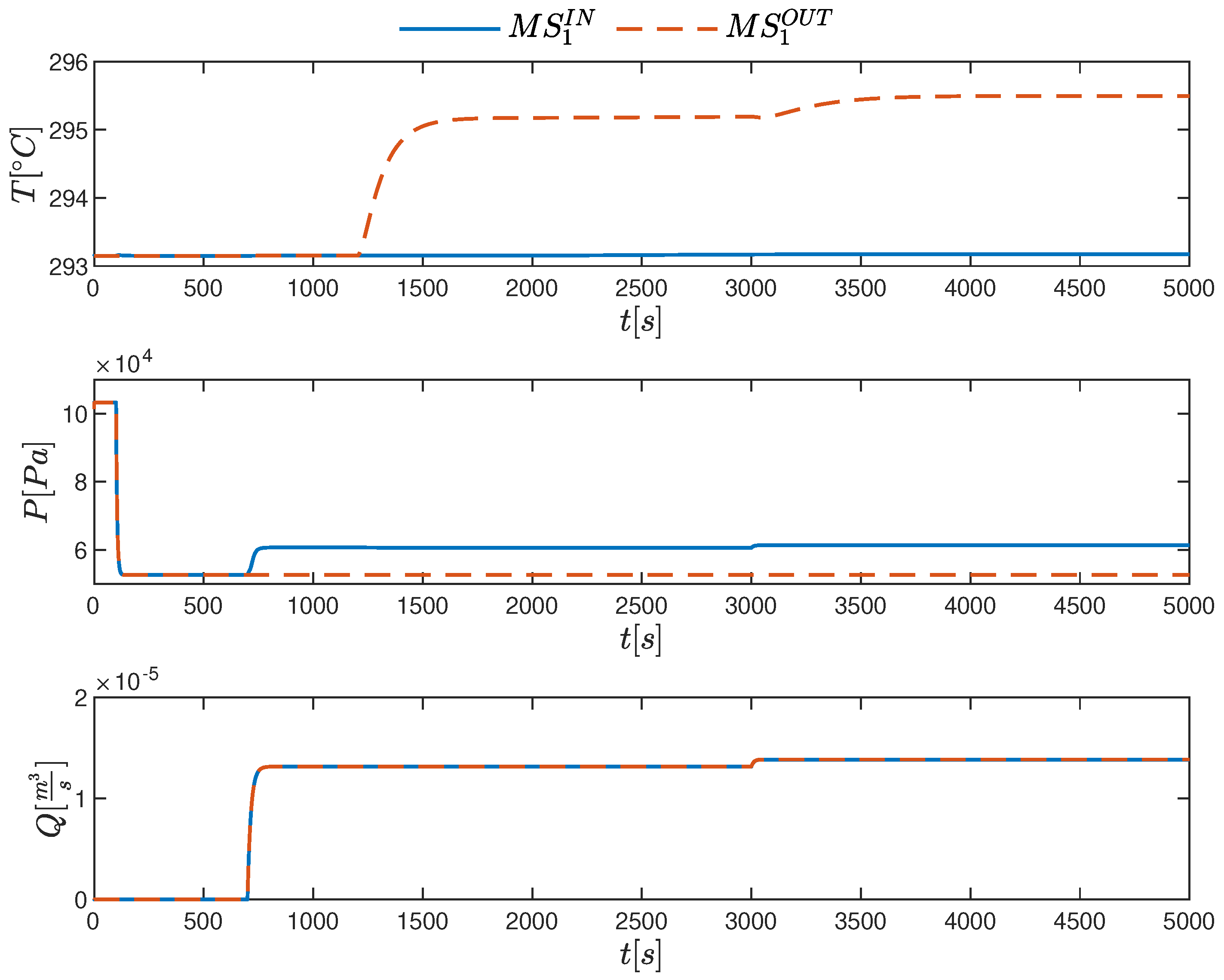
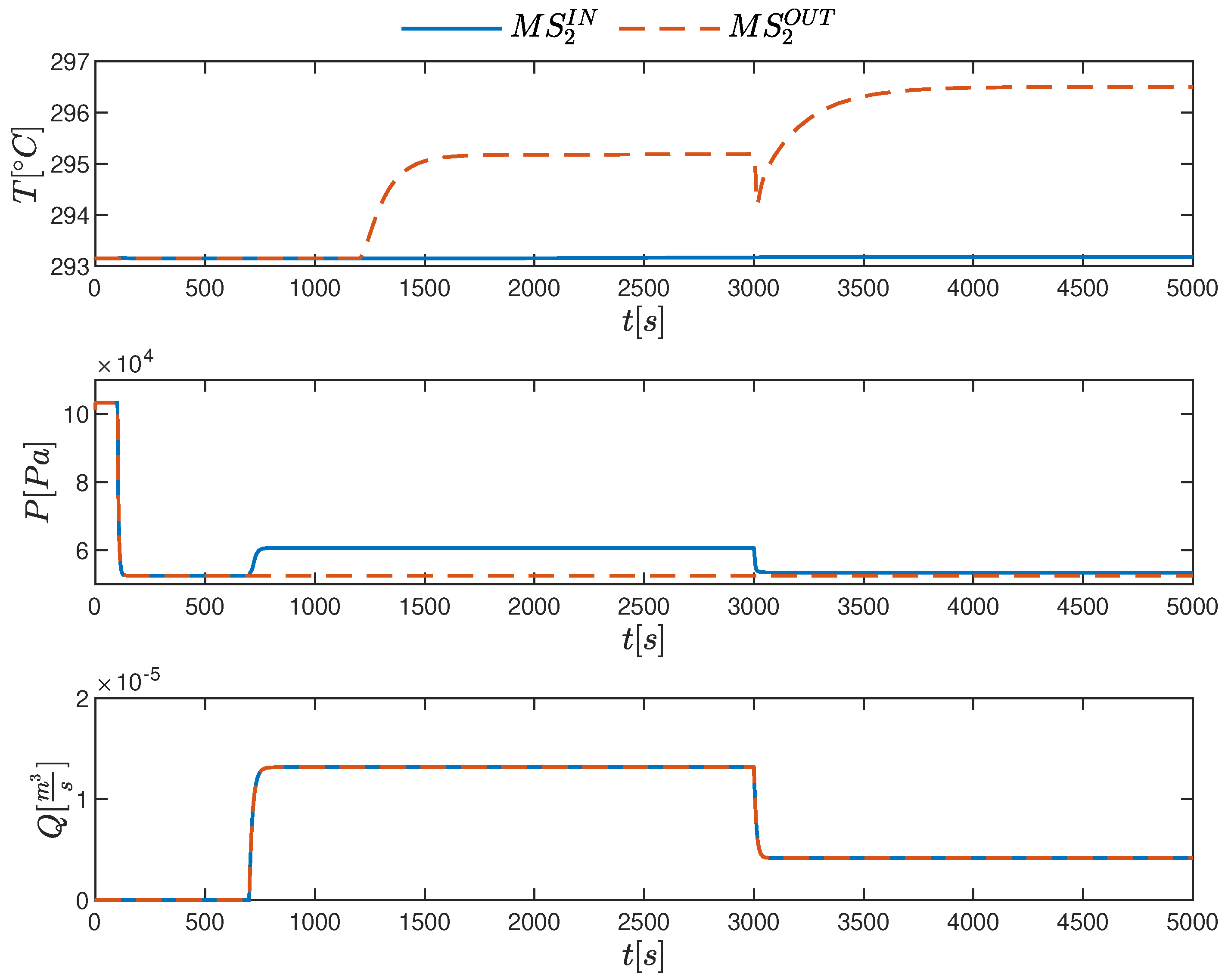
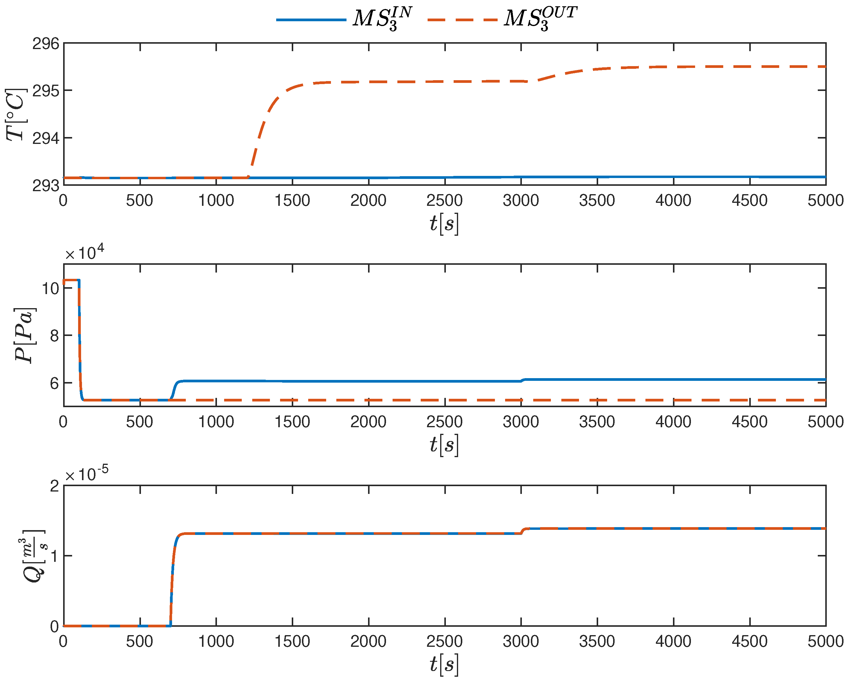
Figure 23. The first change is connected with turning on the pressure pump to achieve leak-less. Then, the main liquid flow pump is turned on and we can observe the rise of the pressure, but it is still under atmospheric pressure. Next, there is a change in valve before one stave and we can observe pressure changes. Finally, the valve is opened to the maximum and the last thing is to turn on the electronics to observe the liquid heat process.
Simulation results presenting the temperature change are shown in
Figure 20,
Figure 21,
Figure 22 and
Figure 23. We can observe in the final stage of simulation that the ideal change of 2 degrees is achieved due to electronic components simulation. The liquid flow is set to the proper value of staves in simulation and the ideal condition is met.
Simulation results for liquid flow change are shown in
Figure 20,
Figure 21,
Figure 22 and
Figure 23. We can observe the reaction to pump work and then changes of valve positions which varies flow in each section and stave. The results are appropriate and expected for this simulation scenario.
7. Conclusions and Future Research
The digital twin approach allows help in the design and the extension of the hardware and software objects used in a high-energy physics experiment. The work is performed for a not-yet existing thermal system. The process was modeled using MATLAB, Simulink and Simscape environments using design structures and parameters. Next, it was equipped with a digital twin control system, which included a PLC controller and SCADA supervisory system. Control structures were proposed and validated. Therefore, future system realization is made easier mitigating project risks.
This work reports that using a digital twin-based approach can develop a general control system structure of a non-existing process. Process parameters are known only approximately. Therefore, although the controllers’ parameters have been tuned for the assumed model, it is expected that precise tuning will be carried out when the real process is available.
Author Contributions
Conceptualization, A.W., P.D.D., M.C., M.K., M.Ł., R.N., S.P., K.R. and K.Z.; methodology, A.W., P.D.D., M.C., M.K., M.Ł., R.N., S.P., K.R. and K.Z.; software, A.W., P.D.D., R.N., S.P. and K.Z.; validation, A.W., P.D.D., R.N., S.P. and K.Z.; formal analysis, A.W., P.D.D., R.N., S.P. and K.Z.; investigation, A.W., P.D.D., R.N., S.P. and K.Z.; resources, P.D.D. and M.Ł.; data curation, A.W., P.D.D., M.C., M.K., M.Ł., R.N., S.P., K.R. and K.Z.; writing—original draft preparation, A.W., P.D.D., M.C., M.K., M.Ł., R.N., S.P., K.R. and K.Z.; writing—review and editing, A.W., P.D.D., M.C., M.K., M.Ł., R.N., S.P., K.R. and K.Z.; visualization, A.W., P.D.D., M.C., M.K., R.N., S.P., K.R. and K.Z.; supervision, P.D.D., M.Ł. and K.R.; project administration, P.D.D., M.Ł. and K.R.; funding acquisition, P.D.D., M.Ł. and K.R. All authors have read and agreed to the published version of the manuscript.
Funding
Studies were funded by IDUB-POB-FWEiTE-1 project granted by Warsaw University of Technology under the program Excellence Initiative: Research University (ID-UB).
Conflicts of Interest
The authors declare no conflict of interest.
Abbreviations
The following abbreviations are used in this manuscript:
| ALICE | A Large Ion Collider Experiment |
| ATLAS | A Toroidal LHC ApparatuS |
| BM@N | Baryonic Matter at Nuclotron |
| CBM | Compressed Baryonic Matter |
| CMS | Compact Muon Solenoid |
| DMC | Dynamic Matrix Control |
| Ecal | Electromagnetic calorimeter |
| FFD | Fast Forward Detector |
| FHCal | Forward Hadron Calorimeter |
| HADES | High Acceptance Di-Electron Spectrometer |
| HMI | Human Machine Interface |
| LHC | Large Hadron Collider |
| MD | Multi Detector |
| MAPS | Active Pixel Sensors |
| P&ID | Piping and Instrumentation Diagram |
| PID | Proportional-Integral-Derivative controller |
| PLC | Programmable Logic Controller |
| RHIC | Relativistic Heavy Ion Collider |
| SCADA | Supervisory Control And Data Acquisition |
| STAR | Solenoidal Tracker at RHIC |
| STD | Silicon Tracking Detector |
| ToF | Time of Flight system |
| TPC | Time Projection Chamber |
| TS | Thermal System |
References
- Barricelli, R.; Casiraghi, E.; Fogli, D. A survey on digital twin: Definitions characteristics applications and design implications. IEEE Access 2019, 7, 167653–167671. [Google Scholar] [CrossRef]
- Mayani, M.G.; Svendsen, M.; Oedegaard, S.I. Drilling digital twin success stories the last 10 years. In Proceedings of the SPE Norway One Day Seminar, Bergen, Norway, 18 April 2018; pp. 1–13. [Google Scholar]
- Poddar, T. Digital twin bridging intelligence among man machine and environments. In Proceedings of the Offshore Technology Conference Asia, Kuala Lumpur, Malaysia, 20–23 March 2018; pp. 1–4. [Google Scholar]
- Uhlemann, T.H.J.; Schock, C.; Lehmann, C.; Freiberger, S.; Steinhilper, R. The Digital Twin: Demonstrating the Potential of Real Time Data Acquisition in Production Systems. Procedia Manuf. 2017, 9, 113–120. [Google Scholar] [CrossRef]
- Mohr, J. Digital Twins for the Oil and Gas Industry; Technical Report; Hashplay Inc.: San Francisco, CA, USA, 2018. [Google Scholar]
- Negri, E.; Fumagalli, L.; Macchi, M. A Review of the Roles of Digital Twin in CPS-based Production Systems. Procedia Manuf. 2017, 11, 939–948. [Google Scholar] [CrossRef]
- Boschert, S.; Rosen, R. Digital Twin-The Simulation Aspect. Mechatron. Future 2016, 59–74. [Google Scholar] [CrossRef]
- Lee, J.; Bagheri, B.; Kao, H. A Cyber Physical Systems architecture for Industry 4.0-based manufacturing systems. Manuf. Lett. 2015, 3, 18–23. [Google Scholar] [CrossRef]
- Lou, X.; Guo, Y.; Gao, Y.; Waedt, K.; Parekh, M. An idea of using Digital Twin to perform the functional safety and cybersecurity analysis. In INFORMATIK 2019: 50 Jahre Gesellschaft für Informatik—Informatik für Gesellschaft (Workshop-Beiträge); Draude, C., Lange, M., Sick, B., Eds.; Gesellschaft für Informatik e.V.: Bonn, Germany, 2019; pp. 283–294. [Google Scholar]
- Turala, M. Silicon tracking detectors—Historical overview. Nucl. Instrum. Methods Phys. Res. A 2005, 541, 1–14. [Google Scholar] [CrossRef]
- Larionov, P. Overview of the silicon tracking system for the CBM experiment. J. Phys. Conf. Ser. 2015, 599, 1–5. [Google Scholar] [CrossRef] [Green Version]
- Larionov, P. Silicon Tracking System (STS) Is the Core Tracking Detector; Goethe University Frankfurt: Frankfurt, Germany, 2015. [Google Scholar]
- Teklishyn, M. The Silicon Tracking System of the CBM experiment at FAIR. EPJ Web Conf. 2018, 171, 21003. [Google Scholar] [CrossRef] [Green Version]
- Herrmann, N. Status and Perspectives of the CBM experiment at FAIR. EPJ Web Conf. 2022, 259, 09001. [Google Scholar] [CrossRef]
- Agakichiev, G.; Agodi, C.; Alvarez-Pol, H.; Atkin, E.; Badura, E.; Balanda, A.; Bassi, A.; Bassini, R.; Bellia, G.; Belver, D.; et al. The High-Acceptance Dielectron Spectrometer HADES. Eur. Phys. J. A 2009, 41, 243–277. [Google Scholar] [CrossRef] [Green Version]
- Kapishin, M. Studies of baryonic matter at the BM@N experiment (JINR). Nucl. Phys. A 2019, 982, 967–970. [Google Scholar] [CrossRef]
- Marx, J.N. The STAR Experiment at RHIC. In Advances in Nuclear Dynamics 2; Springer: Boston, MA, USA, 1996; pp. 233–237. [Google Scholar] [CrossRef]
- Piuz, F.; Klempt, W.; Leistam, L.; De Groot, J.; Schükraft, J. ALICE High-Momentum Particle Identification: Technical Design Report; Technical design report; ALICE, CERN: Geneva, Switzerland, 1998. [Google Scholar]
- Bayatian, G.L.; Chatrchyan, S.; Hmayakyan, G.; Sirunyan, A.M.; Adam, W.; Bergauer, T.; Dragicevic, M.; Ero, J.; Friedl, M.; Fruehwirth, R.; et al. CMS Physics: Technical Design Report Volume 1: Detector Performance and Software; CERN: Geneva, Switzerland, 2006. [Google Scholar]
- Airapetian, A.; Grabsky, V.; Hakopian, H.; Vartapetian, A.; Dick, B.; Fares, F.; Guy, L.P.; Moorhead, G.F.; Sevior, M.E.; Taylor, G.N.; et al. ATLAS: Detector and Physics Performance Technical Design Report; CERN: Geneva, Switzerland, 1999; Volume 1. [Google Scholar]
- Geraksiev, N.S. The Nuclotron-based Ion Collider Facility Project. The Physics Programme for the Multi-Purpose Detector. J. Phys. Conf. Ser. 2018, 1023, 012030. [Google Scholar] [CrossRef]
- Tanabashi, M.; Hagiwara, K.; Hikasa, K.; Nakamura, K.; Sumino, Y.; Takahashi, F.; Tanaka, J.; Agashe, K.; Aielli, G.; Amsler, C.; et al. Review of Particle Physics. Phys. Rev. D 2018, 98, 030001. [Google Scholar] [CrossRef] [Green Version]
- Müller, B. Hadronic signals of deconfinement at RHIC. Nucl. Phys. A 2005, 750, 84–97. [Google Scholar] [CrossRef] [Green Version]
- Aamodt, K.; Quintana, A.A.; Achenbach, R.; Acounis, S.; Adamová, D.; Adler, C.; Aggarwal, M.; Agnese, F.; Rinella, G.A.; Ahammed, Z.; et al. The ALICE experiment at the CERN LHC. JINST 2008, 3, S08002. [Google Scholar] [CrossRef]
- Aamodt, K.; Quintana, A.A.; Achenbach, R.; Acounis, S.; Adamová, D.; Adler, C.; Aggarwal, M.; Agnese, F.; Rinella, G.A.; Ahammed, Z.; et al. Technical Design Report for the Upgrade of the ALICE Inner Tracking System. J. Phys. G 2014, 41, 087002. [Google Scholar] [CrossRef] [Green Version]
- Pelizzari, A. Thermal Fluid-Dynamic Study for the Thermal Control of the New Alice Central Detectors. Master’s Thesis, Universitá Degli Studi di Padova, Padua, Italy, 2017. [Google Scholar]
- Afiz, I.A.; Cunliffe, R.; Alukaidey, T. Mathematical Modeling and Simulation of a Twin-Engine Aircraft Fuel System Using MATLAB-Simulink. Int. J. Control. Sci. Eng. 2018, 8, 1–12. [Google Scholar]
- Das, S. Modeling and Simulation of Mechatronic Systems Using Simscape; Morgan and Claypool: Williston, VT, USA, 2020. [Google Scholar]
- Das, S. Modeling for Hybrid and Electric Vehicles Using Simscape; Morgan and Claypool: Williston, VT, USA, 2021. [Google Scholar]
- MATLAB. Simscape—Model and Simulate Multidomain Physical Systems. Available online: https://www.mathworks.com/products/simscape.html (accessed on 30 September 2021).
- Millerand, S.; Wendlandt, J. Real-Time Simulation of Physical Systems Using Simscape. Available online: https://www.mathworks.com/company/newsletters/articles/real-time-simulation-of-physical-systems-using-simscape.html (accessed on 30 September 2021).
Figure 1.
Silicon tracking detectors in the experiments on the colliders: the beam pipe is marked in green, outer layers are marked in blue, inner layers are labeled in yellow, and the interaction point is marked in red.
Figure 1.
Silicon tracking detectors in the experiments on the colliders: the beam pipe is marked in green, outer layers are marked in blue, inner layers are labeled in yellow, and the interaction point is marked in red.
Figure 2.
Silicon tracking systems in the experiments with the fixed targets: the beam pipe is marked in green, layers of the modules are marked in blue, the dipole magnet is marked in yellow, and the target is marked in red.
Figure 2.
Silicon tracking systems in the experiments with the fixed targets: the beam pipe is marked in green, layers of the modules are marked in blue, the dipole magnet is marked in yellow, and the target is marked in red.
Figure 3.
Simplified P&ID diagram of the thermal system.
Figure 3.
Simplified P&ID diagram of the thermal system.
Figure 4.
Diagram of the system design procedure.
Figure 4.
Diagram of the system design procedure.
Figure 5.
Diagram of the simulated process model. The part of the diagram where the temperature of the liquid is higher is presented with red arrows, while the part where the liquid has a lower temperature is shown with blue arrows.
Figure 5.
Diagram of the simulated process model. The part of the diagram where the temperature of the liquid is higher is presented with red arrows, while the part where the liquid has a lower temperature is shown with blue arrows.
Figure 6.
The thermal system: the base structure.
Figure 6.
The thermal system: the base structure.
Figure 7.
The thermal system: the base structure extended about feed forward.
Figure 7.
The thermal system: the base structure extended about feed forward.
Figure 8.
The thermal system: the advanced structure version 1.
Figure 8.
The thermal system: the advanced structure version 1.
Figure 9.
The thermal system: the advanced structure version 2.
Figure 9.
The thermal system: the advanced structure version 2.
Figure 10.
The chiller simulation.
Figure 10.
The chiller simulation.
Figure 11.
The main pump simulation.
Figure 11.
The main pump simulation.
Figure 12.
The reservoir simulation.
Figure 12.
The reservoir simulation.
Figure 13.
The stave internal structure simulation.
Figure 13.
The stave internal structure simulation.
Figure 14.
The section internal structure simulation.
Figure 14.
The section internal structure simulation.
Figure 15.
The section interconnect structure.
Figure 15.
The section interconnect structure.
Figure 16.
The section internal structure: the control part.
Figure 16.
The section internal structure: the control part.
Figure 17.
The section internal structure: the measurement part.
Figure 17.
The section internal structure: the measurement part.
Figure 18.
The alternative simple structure of sections.
Figure 18.
The alternative simple structure of sections.
Figure 19.
Control signals generation.
Figure 19.
Control signals generation.
Figure 20.
Temperature, pressure and volumetric flow change in the system during the simulation scenario. Measurements have been taken before pump (), after pump (), before the chiller () and after the chiller ().
Figure 20.
Temperature, pressure and volumetric flow change in the system during the simulation scenario. Measurements have been taken before pump (), after pump (), before the chiller () and after the chiller ().
Figure 21.
Temperature, pressure and volumetric flow change in the system during the simulation scenario. Measurements have been taken before the first section () and after the first section ().
Figure 21.
Temperature, pressure and volumetric flow change in the system during the simulation scenario. Measurements have been taken before the first section () and after the first section ().
Figure 22.
Temperature, pressure and volumetric flow change in the system during the simulation scenario. Measurements have been taken before the second section () and after the second section ().
Figure 22.
Temperature, pressure and volumetric flow change in the system during the simulation scenario. Measurements have been taken before the second section () and after the second section ().
Figure 23.
Temperature, pressure and volumetric flow change in the system during the simulation scenario. Measurements have been taken before the third section () and after the third section ().
Figure 23.
Temperature, pressure and volumetric flow change in the system during the simulation scenario. Measurements have been taken before the third section () and after the third section ().
| Publisher’s Note: MDPI stays neutral with regard to jurisdictional claims in published maps and institutional affiliations. |
© 2022 by the authors. Licensee MDPI, Basel, Switzerland. This article is an open access article distributed under the terms and conditions of the Creative Commons Attribution (CC BY) license (https://creativecommons.org/licenses/by/4.0/).


 ,
, 


