Abstract
Complex integrated circuits (ICs) have complex functions and various working modes, which have many factors affecting the performance of a single event effect. The single event effect performance of complex ICs is highly program-dependent and the single event sensitivity of a typical operating mode is generally used to represent the single event performance of the circuits. Traditional evaluation methods fail to consider the cross effects of multiple factors and the comprehensive effects of each factor on the single event soft error cross section. In order to solve this problem, a new quantitative study method of single event error cross section based on a generalized linear model for different test programs is proposed. The laser test data is divided into two groups: a training set and a validation set. The former is used for model construction and parameter estimation based on five methods, such as the generalized linear model and Ensemble, while the latter is used for quantitative evaluation and validation of a single event soft error cross section of the model. In terms of percentage error, the minimum mean estimation error on the validation set is 13.93%. Therefore, it has a high accuracy to evaluate the single event soft error cross section of circuits under different testing programs based on the generalized linear model, which provides a new idea for the evaluation of a single event effect on complex ICs.
1. Introduction
With the rapid development of aerospace technology and deeper exploration in space, the requirements for performance of spacecraft are also increasing. Correspondingly, the reliability and the radiation-hardened performance of complex integrated circuits (ICs) are facing higher requirements [1]. Nowadays, with the reduction in the process size of semiconductor devices, the single event effect (SEE), is seriously affecting the safety of space missions, which is becoming more and more significant [2]. Therefore, it is necessary to evaluate the SEE sensitivity of complex ICs before they are applied to space missions [3]. At present, the SEE evaluation methods of ICs recognized by the industry mainly include a heavy ion test, a proton test, and other radiation tests. The SEE sensitivity of complex ICs has a strong program dependence on which different users have different concerns and applications, so the test programs cannot be traversed. In addition, due to the limited time and high cost of the heavy ion accelerator, it is not suitable for all ICs to carry out radiation tests. Therefore, several simulation methods and fault injection methods have been used to study the SEE sensitivity of complex ICs.
VSenek et al. [4] proposed a Single Event Upset (SEU) simulation prediction method based on the duty cycle to predict the SEU cross section of processors under different test programs. A simple error rate prediction model was preliminarily established. However, the method of analyzing the duty factor was difficult to be applied to complex applications, such as programs with conditional branches. Emmanuel et al. [5] carried out the SEU simulation on processor under different programs based on fault injection, and applied a new fault model of multi-fault injection to dual-fault injection. The model was designed to represent a possible non-concurrent radiation-induced soft error, which was only useful for specific processors in this paper. Gao jie, li qiang et al. [6] studied the relationship between the dynamic and the static SEU rates of satellite microprocessors by using the concept of program duty ratio and fault injection technology, which verified only by fault injection but not by radiation experiments. Zhao Yuanfu et al. [7] proposed a method to predict the SEE of complex ICs, which required a detailed analysis of different test programs and a large amount of work. The prediction method has been verified by radiation experiments, which has a good guiding significance.
The simulation method needs to establish different models for different circuits, which is complicated and time-consuming, and the simulation results have relatively large errors compared with the real test results. The method of fault injection has some problems of precision, accuracy, and speed for the modeling. None of the above methods have taken the cross influence of multiple factors and the comprehensive influence and accurate quantification of SEE soft error cross section into account.
In view of the above shortcomings, laser SEE test data as small sample training set has been used for modeling based on the generalized linear model. Quantitative evaluation on the SEE cross section of the circuit under different test programs has been conducted and the evaluation errors of training set and validation set under different methods are verified, and they have been compared. It provides a new idea for the evaluation of SEE soft error cross section in complex ICs. The SEU cross section of devices under different test programs can be predicted by the new method without carrying out radiation tests on all test modes. It can effectively solve the problem of evaluating the radiation performance of complex ICs under different test modes and obtain high accuracy.
2. Circuit Descriptions and Radiation Experiments
2.1. Circuit Description
The research object is a 32-bit radiation-hardened microprocessor, which has all the typical characteristics of complex ICs, such as large scale, high frequency, multiple modules and complex functions. The system-level error detection and correction are adopted by the radiation-hardened microprocessor. The circuit consists of an integer processing unit (IU), a floating point processing unit (FPU), CACHE, register (REGFILE), a debugging support unit (DSU), a serial port (UART), a storage/interrupt controller, a watchdog, a timer, and other units, which realize data interaction through AMBA bus. The functional block diagram of a microprocessor is shown in Figure 1.
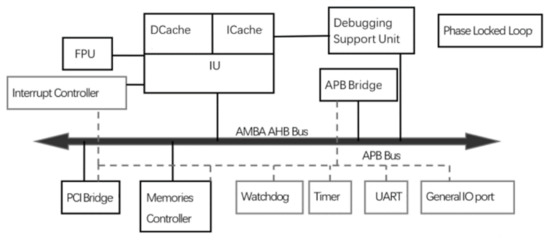
Figure 1.
Functional block diagram of the microprocessor.
2.2. Experiment Setting
In this paper, a set of function test programs is developed to simulate the typical function state of a user, which makes the CPU instruction coverage reach 100%, and it also covers all the logic units of the circuit. Taking P1–P4 test programs as the training test, they perform a single-precision integer operation and a double-precision floating point operation in the CACHE open and closed states, respectively, which cover eight standard test functions. P1 is a single-precision integer operation in CACHE ON mode, P2 is a single-precision integer operation in CACHE OFF mode. P3 is the double-precision floating-point operation in CACHE ON mode, and P4 is the double-precision floating-point operation in CACHE OFF mode. P5–P8 test programs are designed as validation test programs. In order to better verify the effectiveness of the model, this validation program has randomness, and it does not require instruction coverage and logical unit coverage. The processor will continuously access Refile data when executing different test programs. The statistics of register usage of the target circuit under eight different test programs are shown in Table 1.

Table 1.
Statistics of register usage under eight test programs.
2.3. Radiation Experiments
The single event upset soft error cross sections (SEU cross sections) of the circuit under different test programs are obtained by pulse laser test [8]. During the test, the working voltage of the target circuit is set as the lowest level, where IO voltage is 2.97V and core voltage is 1.62 V. The backside irradiation laser test is carried out using PL2210A-P17 pulsed laser with 100 Hz frequency. The laser SEE test site is shown in Figure 2. The laser test data of the training set is shown in Table 2, and the laser test data of the validation set is shown in Table 3 in which the effective laser energy (i.e., laser energy focused in the active region ) has been equivalent to the LET value of heavy ion [9].
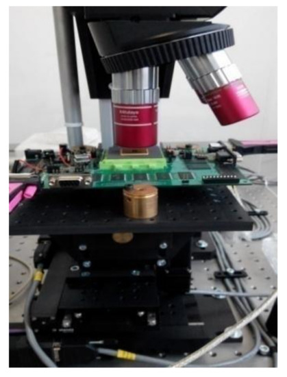
Figure 2.
Laser SEE test site.
Table 2.
Laser SEE soft error cross section of Training set (10−7 errors/cm2).
Table 3.
Laser SEE soft error cross section of validation set (10−7 errors/cm2).
The conversion relation between the initial laser energy and the LET value of the heavy ion is shown in Formula (1):
where f is the effect factor of the spot, R is the reflectance of the device surface, is the metal layer reflectance of the device, is the silicon substrate absorption coefficient of the device and its measured value, and h is the Planck constant.
Four validation programs for P5–P8 were designed, and laser tests were carried out under different laser energies, respectively. The obtained laser test data of P5–P8 are shown in Table 3.
3. Modeling and Parameter Estimation
Compared with the data obtained by software simulation, the laser test data is closer to the radiation sensitivity of the circuit in the actual radiation environment, so the model established based on laser test data have a higher accuracy. There are 16 observations of laser test data, which are typical small sample data, and the use of second-order and above polynomial or tree models may lead to overfitting [10,11,12]. The generalized linear model is linear with respect to the unknown parameters, but nonlinear with respect to the known variables. The nonlinear functional relational quantization model between the independent variable and the dependent variable can be established based on the linear parameters and multiple bases. The corresponding model has a good fitting effect and prediction accuracy. Therefore, the pulsed laser SEE test data of P1–P4 as the training set are used to build the model based on the generalized linear model. Four methods of generalized least squares method [10,11], the weighted least squares estimation method [13], the median regression method [12], and the least trimmed squares method [12] are used to obtain the estimation parameter of the generalized linear model. The four methods mentioned above are combined with optimal weights, namely the Ensemble method as the fifth method. Then, a laser test is performed on the target circuit under the P5–P8 validation programs, and the obtained laser test data is used as the validation set to verify the generalized linear model. The flow chart of the method to quantitatively evaluate the SEE soft error cross section of complex ICs based on the generalized linear model is shown in Figure 3.
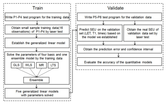
Figure 3.
The flow chart of the method.
Firstly, the P1–P4 test program for the training set is written, and 16 groups of small sample test data are obtained by laser test. The test data is used as the training set for the generalized linear model. Then, GLS, WLS, MR, LTS, and Ensemble methods are established and parameters are optimized on the target functions. The P5–P8 test programs as the validation set are written and then the generalized linear model is used to predict the SEE soft error cross section. Meanwhile, the soft error cross section under radiation is obtained by laser test. By evaluating the prediction error and the confidence interval on the test data, the precision of the quantitative prediction model is obtained.
3.1. Model Building
The generalized linear model is established using Formula (2).
Formula (2) represents the quantitative relationship between SEU and its impact factor, such as . Since the value of the SEU soft error cross section must be positive, and the right side of the equation takes the value of the entire real number domain, we take the logarithm of the SEU and put it into the model, that is, taken as the link function of Poisson regression. The model is linear with respect to unknown parameters, but nonlinear with respect to several known independent variables. Here, the function can be made of any nonlinear function about independent variables according to your observations and assumptions, such as neural networks, GBDT (gradient boosting decision tree), spline functions, or polynomials about independent variables, etc. [10,11]. In this paper, is taken as each independent variable itself to minimize the number of parameters to prevent overfitting and to achieve better predictions. The simulation software used for modeling and parameter estimation in this paper is R-3.5.3.
At this point, the above model can be simplified to Formula (3)
Among them, , is the number of experiments, which is 16 in this paper, and is a column vector of length n. Each column of is the number of registers read times (times), program execution cycle (T1), average register access time (T2), LET and an intercept term (I) that is all 1, each row of is an observation data. The dimension of matrix is . is the unknown parameter column vector of length 5 to be solved, and is the measurement error column vector of length .
3.2. Variable Selection
There are multiple criteria such as , AIC, and BIC for variable selection of the model [11]. In this paper, AIC criterion is chosen for variable selection, which is the sum of the negative average log-likelihood and the penalty term considering the number of parameters. The lower the value, the better the prediction effect of the model. The result of variable selection using the AIC criterion is shown in Figure 4.
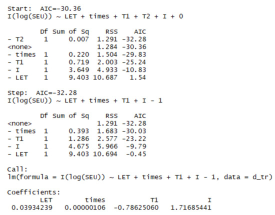
Figure 4.
Variable selection using AIC criteria.
As can be seen from Figure 3, the final result of variable selection retains the number of register reads (times), program execution cycle (T1), LET and the intercept term (I) that is all 1, and it excludes the average register access time (T2).
3.3. Parameter Estimation
For different assumptions of measurement error or different loss functions, different parameter estimates and predicted values of SEU cross section can be obtained. In order to further analyze the experimental data and to obtain a more accurate and robust model, the following four methods are firstly used to carry out model building, in which the first two are based on the Gaussian distribution assumption, and the latter two are robust parameter estimation methods, both of them are used to solve Formula (3), and is the estimated value of . Methods for parameter estimation are shown in Table 4.
Table 4.
Methods for parameter estimation.
The estimation parameter for the training set obtained by the above four methods are shown in Table 5. It can be seen that the influence coefficients of LET and times obtained by different methods are positive, while T1 is on the contrary, and the values of the four methods are relatively close, that is, they increase with the growing of LET and times and decrease with the increase of T1.
Table 5.
Estimation parameters for training set under different methods.
3.4. Model Optimization
Considering that each of the four methods in Section 3.3 may have advantages and disadvantages, the Ensemble method [10,11], which performs optimized linear weighting on the predicted values of these four methods by minimizing the combined variance, is adopted to reduce the prediction variance, shrink the confidence interval, and make predictions more robust. It can be seen from Formula (4) that after Ensemble, the variance of the forecast value, which is the weighted average of the evaluation from the four methods mentioned above, is reduced to minimize and thus becomes more reliable.
is the covariance matrix of the evaluation errors of the four methods.
The covariance matrix of these four methods in Section 3.3 calculated based on the training dataset is shown in Table 6, where the diagonal is the variance of the evaluation errors of the four methods. It can be seen that the evaluation variances of the two robust parameter estimation methods, MR and LTS, are all less than 50, which means the standard deviation of the evaluation errors of the SEU cross section prediction value is less than . The covariance of the WLS method and the LTS method is the smallest, which is −2.9, thus the correlation coefficient of these two is . The negative correlation of these two is used by the Ensemble method to further reduce the evaluation error variance of SEU.
Table 6.
Covariance matrix of the evaluation errors of the four methods.
The inner point method of constraint optimization algorithm [12,13] is used to calculate the optimal weights . It can be seen that MR method has the largest weight, while GLS method has almost zero weight.
3.5. Evaluation Error
In order to verify the evaluation performance of the model on the test data, the above five evaluation methods are used in the training set and the validation set to verify the evaluation effect of the model, respectively. For the evaluation of error, root mean square error (RMSE) [10,11], average error percentage, and other various evaluation indicators are selected. The smaller the value, the smaller the evaluation error and the higher the evaluation accuracy. The evaluation errors of the training set and the validation set under different methods are shown in Table 7.
Table 7.
Evaluation errors of training set and validation set under different methods.
Taking RMSE [10,11], the most commonly used evaluation method, as an example, Ensemble and the MR method have relatively low RMSE in the training set and the validation set, while the other three methods have relatively large evaluation errors in validation set. The MR method, as one of the robust parameter estimation methods, shows a lower evaluation error in the training set and the validation set compared with the GLS and the WLS methods based on Gaussian distribution, indicating that the error of SEU data collected in the experiment may be non-Gaussian distribution, or Gaussian characteristics are not obvious due to small samples. It also verified the reliability of the MR and the Ensemble methods in data modeling, that is, the quantitative evaluation model established by us is effective, and it has a certain accuracy.
4. Confidence Interval Analysis
In the above section, the evaluation errors are compared. Considering the quantity of data is small, the performance of five methods can be affected by accidental data, therefore in this section further analysis on the confidence interval is carried out. The shorter confidence interval means a smaller evaluation error variance and a higher reliability. So, in this section, further comparison of confidence interval with five methods is performed.
In this paper, the bootstrap method based on statistical sampling is used to calculate the confidence interval of SEU cross section. Multiple SEU cross sections can be obtained by repeated sampling with replacements. The bootstrap times in this paper is set as B = 300.
Figure 5, Figure 6, Figure 7 and Figure 8 show the evaluation value and a 95% confidence interval of the five methods on the training set and the validation set, respectively. The evaluation error is the difference between the evaluation value and the soft error cross section value observed in the laser experiment. Gray bars representing known experimental values, points and line segments of five colors are the respective evaluation values and confidence intervals of the five methods. The narrower the confidence interval is, the higher the evaluation accuracy is. Figure 7 and Figure 8 show the probability density function of the evaluation error of the five methods on the training set and validation set, which is calculated using kernel method (gaussian kernel is used, bandwidth is determined based on cross-validation). It can be seen that the value of the error corresponding to the highest density of Ensemble and MR methods on the validation set is concentrated near zero, but the former is more concentrated at zero than the latter. The error distribution of the other three methods is relatively flat, and the error corresponding to the highest probability density is far from zero. As can be seen from Figure 5, Figure 6, Figure 7 and Figure 8 and Table 7, the Ensemble method has the best evaluation accuracy RMSE and the narrowest confidence interval in the validation set, which can be used to evaluate the SEE soft error cross section based on different test programs and laser energy.
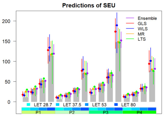
Figure 5.
Evaluations, 95% confidence intervals and real values of the five methods on the training set.
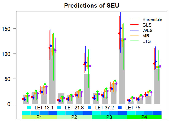
Figure 6.
Evaluations, 95% confidence intervals and real values of the five methods on the validation set.
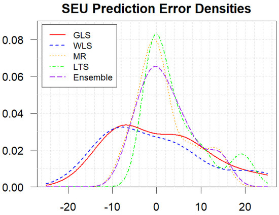
Figure 7.
Density function of evaluation errors of five methods on training set.
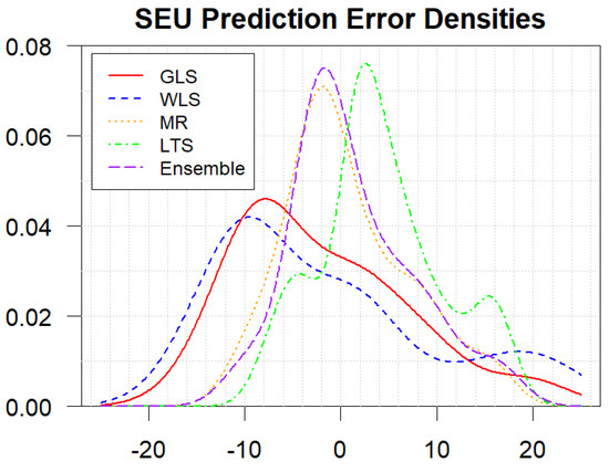
Figure 8.
Density function of evaluation errors of five methods on validation set.
5. Conclusions
A new method based on the generalized linear model for quantitative evaluation of a SEE soft error cross section under different test programs is presented. Different test programs are designed, and the data sets of a laser test under several test programs and register calls of different test programs are divided into training and validation groups. The training set is used for modeling and parameter estimation of the five methods, and the validation set is used to evaluate the model accuracy. The evaluation value, evaluation error, 95% confidence interval, and the probability density function of the five methods on the training set and the validation set are computed. The results show that the quantitative evaluation method of complex ICs based on generalized linear models can achieve a high accuracy of 13.93%. Various factors of the SEE sensitivity of comprehensive effect and quantitative evaluation are considered in the evaluation method. Quantitative evaluation is suitable for small sample experiment data under different test programs, which is an applicable innovation.
Author Contributions
Conceptualization, F.C. and H.C.; methodology, F.C.; software, C.Y. and L.Y.; validation, F.C., L.W. and Y.L.; formal analysis, F.C.; investigation, F.C. and C.Y.; resources, C.Y.; data curation, L.Y.; writing—original draft preparation, F.C. and Y.L.; writing—review and editing, H.C. and L.W.; visualization, L.Y.; supervision, C.Y.; project administration, F.C. and H.C.; funding acquisition, F.C. All authors have read and agreed to the published version of the manuscript.
Funding
This research received no external funding.
Conflicts of Interest
The authors declare no conflict of interest.
References
- Chen, R.; Zhang, F.; Chen, W.; Ding, L.; Guo, X.; Shen, C.; Luo, Y.; Zhao, W.; Zheng, L.; Guo, H.; et al. Single-Event Multiple Transients in Conventional and Guard-Ring Hardened Inverter Chains Under Pulsed Laser and Heavy-Ion Irradiation. IEEE Trans. Nucl. Sci. 2018, 64, 2511–2518. [Google Scholar] [CrossRef]
- Raine, M.; Hubert, G.; Gaillardin, M.; Artola, L.; Paillet, P.; Girard, S.; Sauvestre, J.-E.; Bournel, A. Impact of the Radial Ionization Profile on SEE Prediction for SOI Transistors and SRAMs Beyond the 32-nm Technological Node. IEEE Trans. Nucl. Sci. 2011, 58, 840–847. [Google Scholar] [CrossRef]
- Huang, P.; Chen, S.; Chen, J.; Liang, B.; Chi, Y. Heavy-Ion-Induced Charge Sharing Measurement with a Novel Uniform Vertical Inverter Chains (UniVIC) SEMT Test Structure. IEEE Trans. Nucl. Sci. 2015, 62, 3330–3338. [Google Scholar] [CrossRef]
- Asenek, V.; Underwood, C.; Velazco, R. SEU induced errors observed in microprocessor systems. IEEE Trans. Nucl. Sci. 1998, 45, 2876–2883. [Google Scholar] [CrossRef]
- Touloupis, E.; Flint, A.; Chouliaras, V.A. Study of the Effects of SEU-Induced Faults on a Pipeline-Protected Microprocessor. IEEE Trans. Comput. 2007, 56, 1585–1596. [Google Scholar]
- Gao, J.; Li, Q. An SEU rate prediction method for microprocessors of space applications. J. Nucl. Tech. 2012, 35, 201–205. [Google Scholar]
- Yu, C.Q.; Fan, L. A Prediction Technique of Single Event Effects on Complex Integrated Circuits. J. Semicond. 2015, 36, 115003-1–115003-5. [Google Scholar]
- Buchner, S.P.; Miller, F.; Pouget, V.; McMorrow, D.P. Pulsed-Laser Testing for Single-Event Effects Investigations. IEEE Trans. Nucl. Sci. 2013, 60, 1852–1875. [Google Scholar] [CrossRef]
- Shangguan, S.P. Experimental Study on Single Event Effect Pulsed Laser Simulation of New Material Devices. Ph.D. Thesis, National Space Science Center, The Chinese Academy of Sciences, Beijing, China, 2020. [Google Scholar]
- Murphy, K.P. Machine Learning: A Probabilistic Perspective; MIT Press: Cambridge, MA, USA, 2012. [Google Scholar]
- Hastie, T.; Tibshirani, R.; Friedman, J. The Elements of Statistical Learning, 2nd ed.; Springer: Berlin/Heidelberg, Germany, 2009. [Google Scholar]
- Rousseeuw, P.J.; Hampel, F.R.; Ronchetti, E.M.; Stahel, W.A. Robust Statistics: The Approach Based on Influence Functions; John Wiley & Sons: Hoboken, NJ, USA, 2011. [Google Scholar]
- Jun, S. Mathematical Statistics, 2nd ed.; Springer: Berlin/Heidelberg, Germany, 2003. [Google Scholar]
Publisher’s Note: MDPI stays neutral with regard to jurisdictional claims in published maps and institutional affiliations. |
© 2022 by the authors. Licensee MDPI, Basel, Switzerland. This article is an open access article distributed under the terms and conditions of the Creative Commons Attribution (CC BY) license (https://creativecommons.org/licenses/by/4.0/).