A Novel Carrier Tracking Approach for GPS Signals Based on Gauss–Hermite Kalman Filter

Abstract

In a conventional GPS receiver, the carrier tracking system is the key stage that keeps the receiver locked to the radio navigation parameters (RNPs) of the received signal. The most commonly used approaches to the tracking system are phase lock loop (PLL), frequency lock loop (FLL), and FLL-assisted PLL. The main limitation of the above approaches is that their performance deteriorates when working with weak signals and in harsh environments. In recent years, Kalman filter (KF)-based tracking loop architectures have gained increased attention due to their robust and better performance compared with conventional architectures. In this paper, a novel Gauss–Hermite Kalman filtering-based carrier tracking algorithm is proposed for static and moving receivers with weak GPS signals. The performance of the proposed algorithm is compared with two other approaches: extended Kalman filter (EKF) and unscented Kalman filter (UKF). Simulations were conducted using a software-defined GPS simulator and software device radio (SDR) modules. A comparative analysis of the tracking methods demonstrated that the proposed tracking method shows a better performance and improves the tracking sensitivity and capability under weak signal conditions as compared with EKF- and UKF-based tracking methods. In addition, the results show that the proposed approach improves the Doppler frequency measurement accuracy under dynamic operation conditions.

1. Introduction

During recent years, the use of Global Positioning Systems (GPSs) has remarkably increased, thus increasing the demand for accurate navigation and timing services. These requirements have led to the fact that a special role is assigned to research in the field of GPS receiver technology, facing new challenges such as the operation of GPS receivers in a high-noise environment, e.g., in urban, forest and indoor areas.

In conventional GPS receivers, digital processing is based on the channel structure. Each channel is designed to process data from a single GPS satellite, including acquisition, tracking, demodulation of navigation data, and solving the navigation solution.

In traditional GPS signal tracking approaches, there are three kinds of tracking loop: phase tracking loop (PLL), frequency lock loop (FLL), and delay lock loop (DLL). These loops estimate the following radio navigation parameters (RNPs): carrier phase, Doppler frequency, and code phase, respectively [1,2,3,4]. Since the above approaches use maximum-likelihood estimation, the accuracy of the RNP estimate is low [2,5]. In recent years, a different approach to tracking GPS signals based on Kalman filtering has been investigated. It is known that a linear Kalman filter (LKF) is the optimal solution for the Bayesian problem [6]. In an LKF-based tracking system, the optimal tracking filter, i.e., the LKF, replaces the tracking loop filter. In this case, the outputs of the loop discriminators are used as measurements. According to the literature, the KF-based tracking system shows superior tracking performance. The authors of [7] proposed an explicit tuning investigation and validation of a full KF-based tracking loop in GNSS receivers. In [8], a multifrequency carrier tracking architecture based on the LKF was proposed to improve the robustness and accuracy of carrier tracking loop in frequency-selective fading environments. This architecture combines a traditional single frequency-independent tracking mode, which only uses measurements from a single carrier, a multifrequency joint tracking mode, which linearly combines measurements from multiple carriers, and a multifrequency optimal tracking mode, which incorporates signal strength in multicarrier combinations via a generalized LKF. In ref. [9], an approach was introduced for designing a system of automated positioning of the engineer reconnaissance devices under high-dynamic-reception conditions with a weak GPS signal. Accordingly, a two-stage carrier tracking system was proposed, which involved both coarse and fine tracking. The first stage was implemented through the use of a conventional scheme, where the PLL and FLL were combined to provide a rough estimate of both the carrier phase and the Doppler frequencies of the received signal. The fine tracking was implemented using LKF, starting after successful bit synchronization. It was demonstrated that the proposed method improved the tracking performance and prevented the bit synchronization loss while simultaneously improving the Doppler frequency measurement accuracy under highly dynamic conditions.

However, the LKF approach assumes that the posteriori probability density at the outputs of discriminators is Gaussian. One disadvantage of this design is that the measurement noise at the discriminator output is not always white Gaussian. This follows from the fact that the use of nonlinear discriminators leads to loss of the white Gaussian property at low values of signal-to-noise ratio [10]. In other words, in the LKF algorithm, the phase estimated accuracy is limited by the nonlinearity of the phase discriminator. This reduces the performance of the LKF when receiving weak signals. In this case, other approaches have been considered that use several different strategies for approaching the optimal solution. These approaches are suboptimal and include the extended Kalman filter (EKF) and unscented Kalman filter (UKF) [11,12,13,14,15,16,17,18,19]. In this variant, a suboptimal nonlinear tracking filter (EKF or UKF) replaces both the discriminator and the tracking loop filter. In this case, the measurements are the quadrature components of the signals at the outputs of the nonlinear correlators.

The EKF uses the linearization of a nonlinear system by Taylor series expansion. An EKF-based tracking approach was proposed in [11] to address the nonlinearity issue of the phase discriminator in LKF-based tracking system. In [12], a practical implementation and performance assessment of an EKF-based signal tracking loop were presented. In [13,14], an EKF algorithm was proposed to track highly dynamic L1 and L2 GPS signals.

However, the same problem exists in the above algorithms, such as loss of optimality, accuracy reduction, and filter divergence. That is, there is a bias of estimates and errors in the calculation of covariance matrices [6]. An approach [15] based on the extended strong tracking filter (ESTF) was developed to improve the carrier tracking estimation instead of the traditional EKF approach. However, it was concluded that the class of strong tracking filters such as the EKF will suffer the kinds of problems induced by the subjective fading factor.

The UKF is one of the modifications of the sigma-point Kalman filter (SPKF) [6]. That is, the UKF algorithm is based on a set of symmetrically distributed sample points (so-called sigma points), which are used to determine the mean and the covariance [6]. This algorithm gives a more correct solution to nonlinear problems as compared with the EKF and forms suboptimal estimates of the state vector according to the criterion of the minimum mean-square error of the estimate. The authors of [16,17] proposed an SPKF algorithm in the problem of GPS signal parameter estimation in coherent and noncoherent tracking modes in spacecraft autonomous navigation equipment. The obtained results suggested that the SPKF algorithm could form RNP estimates with appropriate accuracy under the conditions of space consumer functioning. The results also demonstrated that the accuracy of the noncoherent tracking mode was worse than that of the coherent tracking system. In [18], a new adaptive unscented Kalman filter (AUKF) was proposed to estimate the RNP of a GPS signal tracking system. The experimental results showed that the proposed AUKF-based method improved the GPS tracking margin by approximately 8 and 3 dB as compared to the conventional algorithm and LKF-based tracking, respectively. The authors of [19] described an additive strong tracking filter using the UKF tracking algorithm for a GPS vector tracking loop. It should be noted that, from a practical point of view, the vector tracking approach requires large computational costs compared to the scalar tracking approach.

However, implementation of the UKF algorithm requires the determination of several coefficients, which are called scaling parameters (α, β, and κ) [6]. It should be noted that not much research effort has been spent on determining if there is a global optimal setting of the UKF scaling parameters [20]. It must also be noted that the choice of the scaling parameter (α) noticeably affects the result of the UKF algorithm. Traditionally, the choice of this parameter is left to the developer. If we follow the recommendations of the authors [6], then α should be chosen as a value other than 0, but as small as possible (α ≤ 0.01). In this paper, the value of this scale parameter was empirically selected as 0.7. With this choice of parameter α, it was possible to improve the quality characteristics of the UKF-tracking based system. This improvement occurred due to a wider spread of sigma points, which led to better consideration of nonlinearities in observations. However, it took several attempts.

Thus, due to the tuning parameters, the rounding errors of numerical calculation for UKF may destroy the non-negative nature and asymmetry of the covariance matrix; thus, the convergence rate of the UKF approach is slow, and the system may also be unstable. Therefore, in order to avoid the influence of scaling parameters on the quality of the UKF algorithm, it is necessary to find other approaches to building a high-quality tracking system instead of UKF.

Recently, other approaches based on statistical processing theory have been proposed to deal with nonlinear systems. A typical example of these novel techniques is the particle filter (PF). PF is a sequential Monte Carlo method based on the Bayesian estimation principle. The PF uses a series of weighted random samples, which are also called particles, to approximate the posterior probability density, so that many kinds of statistical estimates such as the mean and variance can be computed, which makes it capable of dealing with any nonlinear models [6]. In [21,22], PF-based carrier tracking approaches were proposed for GNSS receivers. However, the main drawback of the PF approach is the lack of computational efficiency [6].

To overcome the problems of low UKF quality and high PF complicity, this paper proposes a new approach to the nonlinear tracking system, which is based on the Gauss–Hermite Kalman filter (GHKF). This approach, which belongs to the family of SPKF, ensures an additional justification of the UKF development and offers further options to improve the accuracy of the approximation. Furthermore, GHKF can provide estimation accuracy comparable to that of a much more computationally intensive simulation-based PF [23]. As a direct quadrature formula, the proposed filter does not need the careful selection of tuning parameters like the UKF [6].

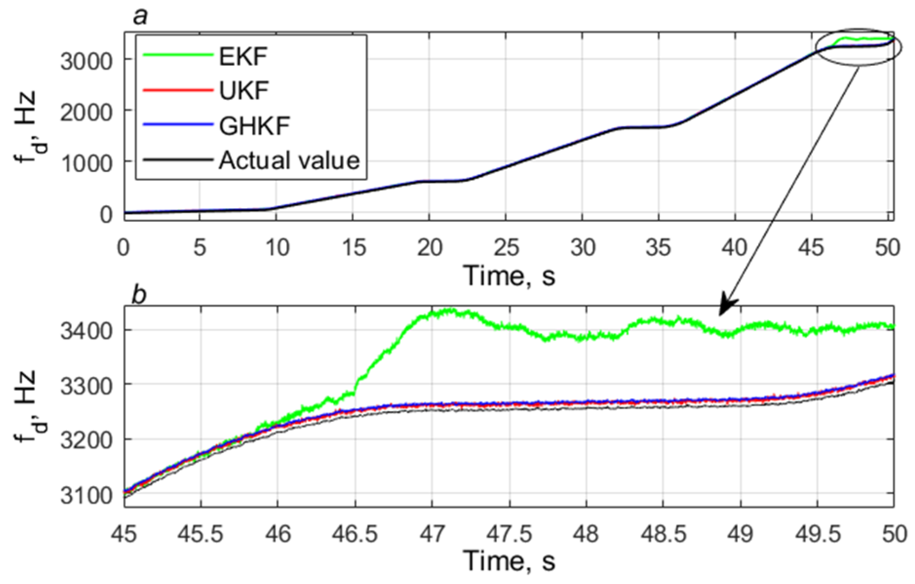
The proposed tracking system was used to estimate the following RNPs of the received GPS signal: amplitude $\widehat{A}$, carrier phase $\widehat{\phi }$, Doppler frequency ${\widehat{f}}_d$, and its change rate ${{\widehat{f}}^{\prime }}_d$.

In the present paper, RNP estimates were compared to those of the EKF- and UKF-based tracking approaches. It should be noted that, in the available literature, there is no performance comparison between nonlinear KF-based tracking loop architectures operating under the same conditions.

The remainder of this paper is organized as follows: in Section 2, the problem description is presented. Then, Section 3 describes the problem solution. In Section 4, the proposed GHKF-based tracking architecture is described in detail. In Section 5, simulations are performed to evaluate the tracking performance and weak dynamic signal performance. Lastly, conclusions are presented in Section 6.

2. Problem Description

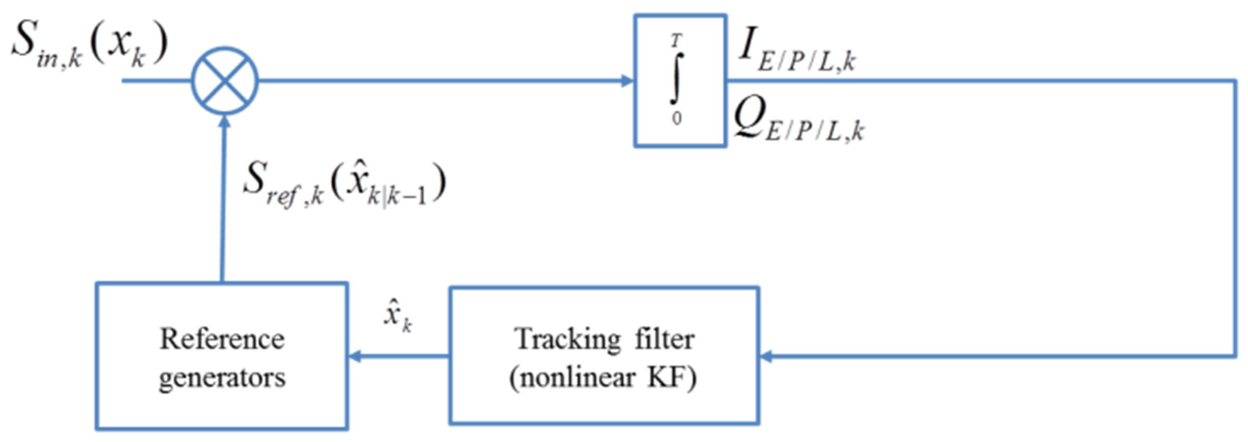
The development of a tracking system based on the Bayesian theory of nonlinear filtering involves setting mathematical models of states and measurements. Figure 1 shows a block diagram of the proposed tracking system model in one channel of the receiver.

This tracking system model can be described as a discrete linear state model with additive white Gaussian noise (AWGN) and a discrete nonlinear measurement model with AWGN [6,13].

$$\{\begin{array}{l}{x}_k=F{x}_{k-1}+u_{x,k-1};\\ z_k=h(x_k)+v_{z,k},\end{array},$$

(1)

where $x_k=[A_k,{\phi }_k,f_{d,k},{f^{\prime }}_{d,k}]$ is the state vector of the RNP of the GPS signal, $F=\left[\begin{array}{cccc}0& 0& 0& 1\\ 1& T& 0.5T^2& 0\\ 0& 1& T& 0\\ 0& 0& 1& 0\end{array}\right]$ is the state transition matrix, $u_{x,k-1}=[n_{A,k-1},n_{\phi ,k-1},n_{f,k-1},n_{f^{\prime },k-1}]$ is a Gaussian distributed process noise with a spectral power density $[q_A,q_{\phi },q_f,q_{f^{\prime }}]$ and a covariance matrix Q, T is the coherent integration time, $z_k=[I_{P,k},Q_{P,k}]$ is the measurement vector at the $k^{th}$ moment, h_k is a nonlinear function of measurements, and $v_{z,k}$ is a Gaussian-distributed measurement noise with a Gaussian probability density function $N(0,R)$. The nonlinear function of measurements h takes the following form [2]:

$$h(x_k)=\{\begin{array}{c}{I}_{P,k}=A_k{R}_{code}\left(\delta {\tau }_k\right)\sin \mathrm{c}\left(f_{d,k}T\right)\cos \left(2\pi (\delta {\phi }_k+\frac{f_{d,k}T}{2}+\frac{{f^{\prime }}_{d,k}{T}^2}{6})\right);\\ Q_{P,k}=A_k{R}_{code}\left(\delta {\tau }_k\right)\sin \mathrm{c}\left(f_{d,k}T\right)\sin \left(2\pi (\delta {\phi }_k+\frac{f_{d,k}T}{2}+\frac{{f^{\prime }}_{d,k}{T}^2}{6})\right),\end{array}$$

(2)

where A_k is the signal amplitude, $R_{code}(\tau )=\{\begin{array}{c}1-\frac{\left|\tau \right|}{T_{chip}}, \left|\tau \right|<T_{chip}\\ 0, \left|\tau \right|>=T_{chip}\end{array}\}$ is the autocorrelation function of the C/A code, $T_{chip}$ is the C/A code chip length ($T_{chip}\approx 1$ µs) [2], $\delta {\tau }_k$ is the code phase error, $\delta {\phi }_k$ is the carrier phase error, $f_{d,k}$ is the carrier Doppler shift, and ${f^{\prime }}_{d,k}$ is the carrier Doppler shift rate. It should be noted that, $\delta {\tau }_k$, in Equation (2), is assumed to be known. In this case, the estimate of $\delta {\tau }_k$ can be taken at the output of the traditional delay lock loop subsystem [1]. The covariance matrix Q of the process noise can be described as follows [2,3,4]:

$$Q={\left(\frac{f_{L1}}{c}\right)}^2{q}_{f^{\prime }}\left[\begin{array}{cccc}0& 0& 0& 0\\ 0& \frac{T^5}{20}& \frac{T^4}{8}& \frac{T^3}{6}\\ 0& \frac{T^4}{8}& \frac{T^3}{3}& \frac{T^2}{2}\\ 0& \frac{T^3}{6}& \frac{T^2}{2}& T\end{array}\right]+\left[\begin{array}{cccc}{q}_{A}T& 0& 0& 0\\ 0& f_{L1}^2(q_f\frac{T^3}{3}+q_{\phi }T)& f_{L1}^2{q}_f\frac{T^2}{2}& 0\\ 0& f_{L1}^2{q}_f\frac{T^2}{2}& T& 0\\ 0& 0& 0& 0\end{array}\right],$$

(3)

where $f_{L1}$ denotes the nominal carrier frequency in Hz ($f_{L1}=1575.420$ MHz for GPS L1 signal), and c denotes the velocity of light. A more detailed description of the process noise spectral power density vector $[q_A,q_{\phi },q_f,q_{f^{\prime }}]$ is presented in [12,13]. The measurement covariance matrix R can be written as follows [2,3,4]:

$$R=\left[\begin{array}{cc}{\sigma }_{IQ}^2& 0\\ 0& {\sigma }_{IQ}^2\end{array}\right]; {\sigma }_{IQ}^2=\frac{N_0}{2T},$$

(4)

where N₀ is the power spectral density of the receiver white noise.

3. Problem Solution

In probability theory, Bayesian estimation is a general probabilistic approach to recursive estimation of an unknown probability density function (PDF) of the state using a mathematical model of the process and a set of receiving measurements. Many problems require an estimation of the state at each receiving measurement. In this case, a recursive filter is a convenient solution. Such a filter consists of mainly two stages: prediction and update. In modern GPS technologies, statistical signal processing methods based on Bayesian filtering theory are widely used. When constructing algorithms for a GPS signal tracking system, it is necessary to describe mathematical models of the system state and measurements. The mathematical model for discrete system state and measurements of a Gaussian process can be described as follows [6]:

$$\{\begin{array}{l}{x}_k=f_k(x_{k-1})+u_{x,k-1},\\ z_k=h_k(x_k)+v_{z,k}.\end{array}$$

(5)

Here, f_k is a possibly nonlinear function of the state $x_{k-1}$, h_k is a possibly nonlinear function of measurements z_k, $u_{x,k-1}$ is an independent and identically Gaussian distributed process noise sequence, and $v_{z,k}$ is an independent and identically Gaussian distributed measurement noise sequence. According to the Bayes method, it is required to form a posteriori PDF $p(x_k|z_{1:k})$ at the moment k, if there is a sequence of all measurements up to the moment k. In this case, it is assumed that the priori PDF $p(x_0|z_0)=p(x_0)$ is known. Then, the PDF $p(x_k|z_{1:k})$ can be obtained recursively in two stages: prediction and update. It is assumed that the required PDF $p(x_{k-1}|z_{1:k-1})$ is known. Then, the prediction stage uses the system model in Equation (5) to obtain the priori pdf of the state at time k using the Chapman–Kolmogorov equation [6].

$$p(x_k|z_{1:k-1})={\displaystyle \int p(x_k|x_{k-1})p(x_{k-1}|z_{1:k-1})d{x}_{k-1}}.$$

(6)

At the timestep k, a new measurement is received, which is used to predict the posterior PDF and implement the update stage using Bayes’ rule.

$$p(x_k|z_{1:k})=\frac{p(z_k|x_k)p(x_k|z_{1:k-1})}{p(z_k|z_{1:k-1})}.$$

(7)

Here, the normalizing constant $p(z_k|z_{1:k-1})$ in Equation (7) has the following form:

$$p(z_k|z_{1:k-1})={\displaystyle \int p(z_k|x_k)p(x_k|z_{1:k-1})d{x}_k}.$$

(8)

It can be seen from Equation (8) that $p(z_k|z_{1:k-1})$ depends on the observation likelihood function $p(z_k|x_k)$ determined by the observation model in Equation (5) and the known statistics of $v_{z,k}$. The recurrence relations in Equations (6) and (7) form the basis for the optimal Bayesian solution of the estimating problem. In practice, solving the Bayesian problem is possible in a number of cases using the Kalman filtering approach. As is known, Kalman obtained a recursive algorithm for generating linear estimates of the state by the criterion of the minimum mean square error for linear models. In this case, the optimal Bayesian estimate ${\widehat{x}}_{k,opt}$ of the state is the posteriori mean value of x_k [6].

$${\widehat{x}}_{k,opt}=E[x_k|z_{1:k}]={\displaystyle \int x_{k}p(x_k|z_{1:k})d{x}_k}.$$

(9)

This algorithm is called the LKF and can be applied for estimating linear dynamical systems by forming Gaussian approximations to the joint distribution of the state x_k and measurement z_k. Therefore, the first and second moments (mean values and covariances) of posteriori estimates are sufficient. In nonlinear systems, other modifications of the traditional KF were considered to find Bayesian estimates of x_k in Equation (9). The most common algorithms for nonlinear filtering problems are EKF and UKF. The EKF extends the scope of KF to nonlinear optimal filtering problems by forming a Gaussian approximation to the nonlinear model using a Taylor series-based transformation. The drawback of this method is the filter divergence in some circumstances [6]. The UKF approach is based on a set of symmetrically distributed sample points used to form the mean and the covariance. There is another approach to selecting the set of sample points for obtaining the mean and covariance. This approach is based on so-called Gaussian filters. In [24], it was shown that the UKF can be considered as a special case of Gaussian filters, where the nonlinear filtering problem is solved using Gaussian-assumed density approximations.

In this paper, we present the GHKF as a Gaussian filtering framework to be used in a GPS carrier tracking system. Next, we conduct a detailed analysis of this filter [6,24,25,26].

In GHKF, the linear equations of KF can be adapted to the nonlinear state space model. Desired moments (mean and covariance) of the original distribution of $x~N(m,P)$ can be obtained exactly by calculating the following integrals [6]:

$$\begin{array}{l}{\mu }_U={\displaystyle \int f(x)N(x|m,P)d{x}_k};\\ S_U={\displaystyle \int \left(f(x)-{\mu }_U\right){\left(f(x)-{\mu }_U\right)}^{T}N(x|m,P)d{x}_k}.\end{array}$$

(10)

These integrals can be evaluated with practically any analytical or numerical integration method. The Gauss–Hermite quadrature rule is a method for solving special integrals of the previous form in a Gaussian kernel with an infinite domain. More specifically, the Gauss–Hermite quadrature can be applied to integrals of the following form:

$${\displaystyle \underset{-\infty }{\overset{+\infty }{\int }}f(x)e^{-x^2}dx}\approx {\displaystyle \sum _{i=1}^p{w}_{i}f(x_i)},$$

(11)

where x_i denotes the sample points (quadrature points), w_i denotes the associated weights to use for the approximation, and p is the number of distinct quadrature points. The quadrature points x_i are chosen to be the zeros of the $p^{th}$-order Hermite polynomial. The Hermite polynomial of degree p is defined as follows:

$$H_p(x)={(-1)}^p\exp (\frac{x^2}{2})\frac{d^p}{d{x}^p}\exp (-\frac{x^2}{2}).$$

(12)

The first two Hermite polynomials are $H_0(x)=1; H_1(x)=x.$ Further polynomials can be found from the following recursion:

$$H_{p+1}(x)=x{H}_p(x)-p{H}_{p-1}(x).$$

(13)

The weights w_i are given by

$$w_i=\frac{2^{p-1}p!\sqrt{\pi }}{p^2{\left[H_{p-1}(x_i)\right]}^2}.$$

(14)

Therefore, one-dimensional Gauss–Hermite quadrature integration refers to the special case of Gaussian quadrature with a unit Gaussian weight function $N(x|0,1)$, i.e., to approximations of the following form:

$${\displaystyle \underset{-\infty }{\overset{+\infty }{\int }}f(x)N(x|0,1)dx}\approx {\displaystyle \sum _{i=1}^p{w}_{i}f(x_i)}.$$

(15)

Now, consider a multidimensional random variable x having a Gaussian density $N(x|0,I_{n_x})$, where n_x is the identity matrix of dimensions $n_x\times n_x$. The one-dimensional integration method can be extended to multidimensional integrals of the following form:

$${\displaystyle \underset{{\Re }^{n_x}}{\int }f(x)N(x|0,I_{n_x})dx}\approx {\displaystyle \sum _{l=1}^k{w}_{l}f({\mathsf{\xi }}_l)}; k=p^{n_x},$$

(16)

where ${\mathsf{\xi }}_l={[{\xi }_l^1,{\xi }_l^2,\dots ,{\xi }_l^{n_x}]}^T$ is the $l^{th}$ column of the quadrature matrix of dimensions $n_x\times k$, which can be described as follows:

$$\xi =\left[{\xi }_1 \dots {\xi }_k\right]=\left(\begin{array}{ccc}{\xi }_1^1& \dots & {\xi }_k^1\\ ⋮& \ddots & ⋮\\ {\xi }_1^{n_x}& \cdots & {\xi }_k^{n_x}\end{array}\right).$$

(17)

Additionally, the weight of the quadrature point vector ${\xi }_l$ can be written as

$$w_l={\displaystyle \prod _{j=1}^{n_x}{w}_l^j}={\displaystyle \prod _{j=1}^{n_x}\frac{2^{p-1}p!\sqrt{\pi }}{p^2{\left[H_{p-1}({\xi }_l^j)\right]}^2}}.$$

(18)

Therefore, if p points are required to calculate the one-dimensional integral, then $k=p^{n_x}$ points are required for the n_x-dimensional case. This set of quadrature points are given by the Cartesian product of n_x vectors, each of which consists of p points. These points are the roots ${\xi }_{1,2,\dots ,p}$ of the Hermite polynomial $H_p(x)$. Thus, the quadrature matrix $\xi$ can be written as

$$\xi ={\left\{{\xi }_1, \dots {\xi }_p\right\}}_1\times {\left\{{\xi }_1, \dots {\xi }_p\right\}}_1\times \dots \times {\left\{{\xi }_1, \dots {\xi }_p\right\}}_{n_x}.$$

(19)

Now, consider a multidimensional random variable x having a Gaussian density $N(x|\mu ,P)$. In this case, the Gaussian multidimensional integral can be written as

$$\begin{array}{l}{\displaystyle \underset{{\Re }^{n_x}}{\int }f(x)N(x|\mu ,P)dx}\\ ={\displaystyle \underset{{\Re }^{n_x}}{\int }f(\mu +\sqrt{P}x)N(x|0,I_{n_x})dx}\approx {\displaystyle \sum _{l=1}^k{w}_{l}f(\mu +\sqrt{P}{\xi }_l)}; k=p^{n_x},\end{array}$$

(20)

where the square root of the covariance matrix $P=\sqrt{P}{\left(\sqrt{P}\right)}^T$ can be obtained by Cholesky factorization.

4. GHKF-Based Carrier Tracking Algorithm

Assume that we have estimate $m_{k-1/k-1}$ of the four-dimensional normally distributed state vector presented in Equation (1) at time k − 1 and its error covariance matrix $P_{k-1}$. The recursive GHKF algorithm of degree p is reduced to the following steps [24,25,26]:

Prediction steps:

• Find the roots $x_i;i=1,2,\dots ,p$ of the Hermite polynomial $H_p(x)$.
• Calculate the corresponding weights, as in Equation (14).
• Use the Cartesian product rule in Equation (11) to expand x_i to a n_x-dimensional case of $p^{n_x}$ points ${\xi }_i; i=1,2,\dots ,p^{n_x}$, with the corresponding weights in Equation (18).
• Propagate the cubature points.

  $${\chi }_{i,k-1|k-1}=m_{k-1|k-1}+\sqrt{P_{k-1|k-1}}{\xi }_i; i=1,2,\dots ,p^{n_x}.$$

  (21)
• Evaluate the cubature points with the dynamic model function, presented in Equation (1).

  $${\chi }_{i,k|k-1}^{*}=F{\chi }_{i,k-1|k-1}.$$

  (22)
• Estimate the predicted state mean and error covariance.

  $$\{\begin{array}{l}{m}_{k|k-1}={\displaystyle \sum _{i=1}^{p^{n_x}}{w}_i}{\chi }_{i,k|k-1}^{*};\\ P_{k|k-1}=\left[{\displaystyle \sum _{i=0}^{2L}{w}_i{\chi }_{i,k|k-1}^{*}{({\chi }_{i,k|k-1}^{*})}^T}\right]-m_{k-1|k-1}{(m_{k-1|k-1})}^T+Q\end{array}.$$

  (23)

Update steps:

• Repeat steps 1–3 from earlier to get the cubature points and their weights.
• Propagate the cubature points.

  $${\chi }_{i,k-1|k-1}=m_{k|k-1}+\sqrt{P_{k|k-1}}{\xi }_i; i=1,2,\dots ,p^{n_x}.$$

  (24)
• Evaluate the cubature points using the measurement model, presented in Equation (2).

  $$z_{i,k-1|k-1}=h({\chi }_{i,k-1|k-1}).$$

  (25)
• Estimate the predicted measurement and the innovation covariance matrix.

  $$\{\begin{array}{l}{\widehat{z}}_{i,k|k-1}={\displaystyle \sum _{i=1}^{p^{n_x}}{w}_i}{z}_{i,k-1|k-1};\\ S_{k|k-1}=\left[{\displaystyle \sum _{i=0}^{2L}{w}_i{z}_{i,k-1|k-1}{(z_{i,k-1|k-1})}^T}\right]-{\widehat{z}}_{i,k|k-1}{({\widehat{z}}_{i,k|k-1})}^T+R.\end{array}$$

  (26)
• Estimate the cross-covariance matrix.

  $$P_{xz,k|k-1}=\left[{\displaystyle \sum _{i=0}^{2L}{w}_i{\chi }_{i,k-1|k-1}{(z_{i,k-1|k-1})}^T}\right]-m_{k|k-1}{({\widehat{z}}_{i,k|k-1})}^T.$$

  (27)
• Calculate the Kalman gain and the current state mean and covariance.

  $$\{\begin{array}{l}{K}_k=(P_{xz,k|k-1}){(S_{k|k-1})}^{-1};\\ m_{k|k}=m_{k|k-1}+K_k(z_k-{\widehat{z}}_{k|k-1});\\ P_k=P_{k|k-1}-K_k{S}_{k|k-1}{K}_k^T.\end{array}$$

  (28)

In the above algorithm, $n_x=4$ is the dimension of the state vector $x_k=[A_k,\delta {\phi }_k,f_{d,k},{f^{\prime }}_{d,k}]$, p is the degree of the Hermite polynomial $H_p(x)$, and Q and R are the covariance matrices of the process and measurement noise, respectively. These matrixes are described in Equations (3) and (4).

5. Simulation Setup and Experiment Results

5.1. Test Setup

To evaluate the proposed algorithm, the tracking algorithm described above was implemented on a software-defined GPS receiver, implemented in Matlab. The receiver directly processes the IF signal, which is read from a data file. The datasets (50 s) were generated using a software-defined GPS simulator, which was implemented using a SDR device, ADALM-PLUTO SDR. The simulator generates GPS baseband signal data streams, which can be converted to RF using the ADALM-PLUTO SDR platform. This simulator is programmed as a 12-channel GPS signal simulator in the L1 (1575, 420 MHz) band. This makes it possible to determine motion patterns of the receiver, taking into account the power of the transmitted signal from each satellite [27]. The RF signal was received by another SDR device, SDRplay RSPdx, and recorded to a data file using a 3 MHz sampling frequency and a 16 bit signal resolution. The experiment setup is shown in Figure 2.

This test was investigated for the evaluation of EKF-, UKF-, and GHKF-based tracking algorithms. Sensitivity of the receiver is an important parameter when comparing the mentioned tracking system algorithms. Tracking sensitivity was evaluated using the carrier-to-noise ratio ($C/N_0$) estimates. $C/N_0$ represents the ratio of the received signal power to the spectral power of the receiver thermal noise in a 1 Hz bandwidth (measured in dB-Hz) and can be written as follows [11,12]:

$$C/N_0=10{\log }_{10}(\frac{{\widehat{A}}^2}{2T{\sigma }_{IQ}^2}).$$

(29)

The tracking threshold of the parameter $C/N_0$ was assumed to be 4 dB-Hz, i.e., the error of $C/N_0$ estimates had to be lower than 4 dB-Hz [12,13]. Similarly, the tracking threshold of the Doppler frequency was assumed to be 25 Hz [12,13]. In this simulation, the coherent integration time was equal to one period of the C/A code, i.e., T = 1 ms. For simplicity, only the performance of PRN 27 satellite is illustrated here.

Table 1. Initial parameters of the proposed tracking system.

Q				Square Roots from Diagonal Elements P0
$q_A$	$q_{\phi }$($\frac{{\mathrm{s}}^2}{\mathrm{Hz}}$)	$q_f$($\frac{1}{\mathrm{Hz}}$)	$q_{f^{\prime }}$($\frac{{{(\mathrm{m}/\mathrm{s}}^3)}^2}{\mathrm{Hz}}$)	${\sigma }_{{\widehat{A}}_0}$	${\sigma }_{{\widehat{\phi }}_0}$ (rad)	${\sigma }_{{\widehat{f}}_{d,0}}$ (Hz)	${\sigma }_{{{\widehat{f}}^{\prime }}_{d,0}}$ ($\frac{\mathrm{Hz}}{\mathrm{s}}$)
${10}^{-3}$	${10}^{-19}$	$8 \times {10}^{-19}$	5	1	$2\pi$	10	20

shows the initial parameters of the three nonlinear algorithms.

In this simulation, the degree of the proposed GHKF was set to 3. At the same time, the UKF scale parameters were empirically chosen as follows: (α = 0.7, β = 2, and κ = 0). Two scenarios of the signal environment were simulated: static and dynamic weak signals. For each scenario, a comparative analysis of the tracking methods was carried out.

5.2. Static Weak Signal Environment Scenario

A scenario of receiving a weak signal in a stationary GPS receiver was simulated. The GPS simulator emulated the controlled, attenuated GPS signals as weak signals. In this scenario the signal power of the satellite PRN 27 remained constant at about 42 dB-Hz until 9 s, and then it decreased by 2.5 dB/s. The minimum power reached 26 dB-Hz in 15 s and was maintained at this level until 34 s. Then, it increased by 2.5 dB/s until 40 s, where it was restored to its original value, before finally remaining constant until 50 s. To compare the sensitivity of the tracking systems, we obtained the $C/N_0$ estimates during the tracking in each algorithm. Figure 3 shows the $C/N_0$ estimates for the three methods.

As can be seen in the figure, the EKF and UKF algorithms could only follow the actual $C/N_0$ value when the signal power was high. When $C/N_0$ reached 26 dB-Hz, the deviation of the $C/N_0$ estimates from the actual value was larger than 4 dB-Hz, especially after 15 s of tracking. In contrast, the GHKF algorithm still correctly estimated the $C/N_0$ parameter until the end of the test. Figure 4 shows the output of the prompt channel correlator, I_p, for a period of 10 s (from 20 to 30 s), when the $C/N_0$ value was below the level of 27 dB-Hz. From the figure, we can see that the EKF-based tracking incorrectly decoded bits of the navigation message; hence, the bit synchronization failed, i.e., there was data bit inversion during the tracking. In this case, the tracking system was unable to serve tracking during the above time interval. Unlike EKF and UKF tracking methods, the GHKF method continued correctly decoding data navigation bits until the end of experiment.

Thus, these results demonstrate that the proposed GHKF tracking algorithm had better performance and improved the tracking sensitivity and capability under weak signal conditions as compared with the EKF- and UKF-based tracking methods.

5.3. Dynamic Weak Signal Environment Scenario

In order to verify the performance of the proposed algorithm for a weak signal under many dynamic conditions, a scenario of a moving receiver was designed with attenuation of the received signal strength. In this case, the signal started at 50 dB-Hz and descended by 0.5 dB/s. The minimum power reached 30 dB-Hz at 50 s. Regarding the dynamic scene simulation, three dynamic periods were simulated with different Doppler rates of 50 Hz/s, 100 Hz/s, and 150 Hz/s. Figure 5 shows the $C/N_0$ estimates with the three tracking algorithms. As can be seen in the figure, the accuracy of the $C/N_0$ estimation, in all algorithms, decreased upon reducing the signal power. It is shown that the EKF algorithm could follow the actual signal strength only when the signal power was high. When the $C/N_0$ reached 32 dB-Hz, the $C/N_0$ estimation showed a large error, and the receiver lost the lock at about t = 45 s. In addition, the $C/N_0$ estimates in the UKF-based tracking algorithm showed a large deviation from the actual value after 45 s of tracking. In contrast, GHKF algorithm still locked the signal, and the $C/N_0$ parameter was correctly estimated with an accuracy of approximately ±2 dB-Hz.

Figure 6 and Figure 7 show estimates of $\widehat{A}$ and ${\widehat{f}}_d$. From these figures, we can see that all algorithms had the same estimate of these RNPs until 45 s of tracking, where $C/N_0=34$ dB-Hz. After that, the EKF algorithm incorrectly estimated the parameters until the end of experiment, where $C/N_0=30$ dB-Hz. For example, it can be noted that, from 46 s onward, at which $C/N_0\approx 33$ dB-Hz, the Doppler frequency obtained in the EKF-based tracking system was determined incorrectly (Figure 7b). Moreover, the amplitude measurement accuracy in the UKF-based tracking algorithm decreased after 45 s of tracking. In contrast, the GHKF algorithm provided the highest tracking stability compared to the other two methods.

6. Conclusions

A GHKF-based tracking system approach was presented in this paper. It was designed to work under conditions of dynamic and weak GPS signal reception. In the proposed approach, a method for forming joint estimates of the RNP in a coherent tracking mode was considered. The performance of the proposed algorithm was evaluated by simulations, using a software-defined simulator and an SDR device. Two nonlinear tracking algorithms were also tested for comparison: EKF and UKF.

The simulation results demonstrated that the proposed algorithm could improve the tracking sensitivity and capability compared with the EKF and UKF methods while simultaneously preventing bit synchronization loss under static weak signal conditions. In addition, under dynamic weak signal conditions, the proposed method was more robust than the other two methods.

The obtained results showed that the GHKF algorithm could form RNP estimates with appropriate accuracy in the proposed static and dynamic scenarios, which are typical for indoor pedestrian and urban vehicle navigation. It is worth mentioning that the tracking performance highly relies on the knowledge of noise statistics. However, the noise covariance is fixed during the GHKF iteration, which may not reflect real variable-noise statistics. Therefore, the adaptive GHKF can be employed in the tracking loop to further improve the tracking performance under more challenging environments.

References

1. Kaplan, E.D.; Hegarty, C.G. Understanding GPS: Principles and Applications, 2nd ed.; Artech House: London, UK, 2006; pp. 164–182. [Google Scholar]
2. Yang, R.; Ling, K.; Poh, E.; Morton, Y. Generalized GPS signal carrier tracking: Part I—Modeling and analysis. IEEE Trans. Aerosp. Electron. Syst. 2017, 53, 1781–1797. [Google Scholar] [CrossRef]
3. Alwin, P.; Benaoumeur, S.; Dong, S.H. Performance Analysis of Sensor Fusion Techniques for Heading Estimation Using Smartphone Sensors. IEEE Sens. J. 2019, 19, 12369–12380. [Google Scholar] [CrossRef]
4. Yin, J.; Tiwari, R.; Johnston, M. Robust GPS Carrier Tracking Model Using Unscented Kalman Filter for a Dynamic Vehicular Communication Channel. IEEE Access 2018, 6, 26930–26938. [Google Scholar] [CrossRef]
5. Niu, X.; Li, B.; Ziedan, N.I.; Geo, W.; Liu, J. Analytical and simulation-based comparison between traditional and Kalman filter-based phase-locked loops. GPS Solut. 2017, 21, 123–135. [Google Scholar] [CrossRef]
6. Sarkka, S. Bayesian Filtering and Smoothing; Cambridge University Press: Espoo, Finland, 2013; pp. 56–114. [Google Scholar]
7. Tang, X.; Chen, X.; Pei, Z.; Wang, P. The Explicit Tuning Investigation and Validation of a Full Kalman Filter-Based Tracking Loop in GNSS Receivers. IEEE Access 2019, 7, 111487–111498. [Google Scholar] [CrossRef]
8. Yang, R.; Xu, D.; Morton, Y.T. Generalized Multifrequency GPS Carrier Tracking Architecture: Design and Performance Analysis. IEEE Trans. Aerosp. Electron. Syst. 2020, 56, 2548–2563. [Google Scholar] [CrossRef]
9. Kanouj, M.M.; Klokov, A.V.; Parvatov, G.N.; Potekaev, A.I. A New Approach to Designing a Positioning System for Operation Under the Conditions of Dynamic Stress and High Noise Level. Russ. Phys. J. 2021, 64, 156–167. [Google Scholar] [CrossRef]
10. Won, J.H.; Pany, T.; Eissfeller, B. Characteristics of Kalman filters for GPS signal. IEEE Trans. Aerosp. Electron. Syst. 2012, 48, 3671–3681. [Google Scholar] [CrossRef]
11. Ziedan, N.I.; Garrison, J.L. Extended Kalman Filter-Based Tracking of Weak GPS Signals under High Dynamic Conditions. In Proceedings of the 17th International Technical Meeting of the Satellite Division of The Institute of Navigation (ION GNSS 2004), Long Beach, CA, USA, 21–24 September 2004; pp. 20–31. [Google Scholar]
12. Tang, X.; Falco, G.; Falletti, E.; Presti, L.L. Practical implementation and performance assessment of an Extended Kalman Filter-based signal tracking loop. In Proceedings of the 2013 IEEE—International Conference on Localization and GNSS (ICL-GNSS), Turin, Italy, 25–27 June 2013; pp. 1–6. [Google Scholar] [CrossRef]
13. Zeng, C.; Li, W. Application of Extended Kalman Filter for tracking high dynamic GPS signal. In Proceedings of the 2016 IEEE—International Conference on Signal and Image Processing (ICSIP), Beijing, China, 13–15 August 2016; pp. 503–507. [Google Scholar] [CrossRef]
14. Zeng, C.; Li, W.; Bi, B.; Chen, Q. Application of Extended Kalman Filter Based Semi-Codeless for Tracking High Dynamic GPS L2 Signal. In Proceedings of the 2017 IEEE—International Conference on Frontiers of Sensors Technologies (ICFST), Shenzhen, China, 14–16 April 2017. [Google Scholar] [CrossRef]
15. Ge, Q.; Shao, T.; Chen, S.; Wen, C. Carrier Tracking Estimation Analysis by Using the Extended Strong Tracking Filtering. IEEE Trans. Ind. Electron. 2017, 64, 1415–1424. [Google Scholar] [CrossRef]
16. Shavrin, V.V.; Tislenko, V.I.; Lebedev, V.Y.; Kondakov, A.S.; Filimonov, V.A.; Kravets, A.P. Quasioptimal estimation of GNSS signal parameters in coherent reception mode using the sigma-point Kalman filter. Gyroscopy Navig. 2017, 8, 24–30. [Google Scholar] [CrossRef]
17. Shavrin, V.V.; Tislenko, V.I.; Lebedev, V.Y.; Konakov, A.S.; Filimonov, V.A. Sigma-Point Kalman Filter Algorithm in the Problem of GPS Signal Parameters Estimation in Non-Coherent Tracking Mode in Spacecraft Autonomous Navigation Equipment. Gyroscopy Navig. 2018, 4, 255–266. [Google Scholar] [CrossRef]
18. Kanouj, M.M.; Klokov, A.V. Adaptive Unscented Kalman Filter for Tracking GPS Signals in the Case of an Unknown and Time-Varying Noise Covariance. Gyroscopy Navig. 2021, 12, 224–235. [Google Scholar] [CrossRef]
19. Lie, S.; Li, S.; Zheng, J.; Wang, Q.; Yuan, Y. C/N0 Estimator Based on the Adaptive Strong Tracking Kalman Filter for GNSS Vector Receivers. Sensors 2020, 20, 739. [Google Scholar] [CrossRef] [Green Version]
20. Merwe, R. Sigma-Point Kalman. Filters for Probabilistic Inference in Dynamic State-Space Models. Ph.D. Thesis, University of Stellenbosch, Stellenbosch, South Africa, 2004. [Google Scholar]
21. Jing, P.; Shaojie, N.; Gang, O. Robust Carrier Tracking Approach for High Dynamic GNSS Signals based on Gaussian Particle Filtering. Int. J. Math. Models Methods Appl. Sci. 2017, 11, 55–60. [Google Scholar]
22. Luan, Z.; Li, Z.; Li, Y. Research on carrier tracking algorithm of low earth orbit satellite based on particle filter. Proc. SPIE 2020, 11373, 113732Z. [Google Scholar] [CrossRef]
23. Sadhu, S.; Srinivasan, M.; Bhaumik, S.; Ghoshal, T.K. Central Difference Formulation of Risk-Sensitive Filter. IEEE Signal Processing Lett. 2007, 14, 421–424. [Google Scholar] [CrossRef]
24. Stecha, J.; Havlena, V. Unscented Kalman filter revisited—Hermite-Gauss Quadrature approach. In Proceedings of the 2012 IEEE International Conference on Information Fusion, Singapore, 9–12 July 2012. [Google Scholar]
25. Ito, K.; Xiong, K. Gaussian filters for nonlinear filtering problems. IEEE Trans. Autom. Control. 2000, 45, 910–927. [Google Scholar] [CrossRef] [Green Version]
26. Elgamoudi, A.; Benzerrouk, H.; Elango, G.A.; Landry, R. Gauss Hermite H∞ Filter for UAV Tracking Using LEO Satellites TDOA/FDOA Measurement—Part I. IEEE Access 2020, 8, 201428–201440. [Google Scholar] [CrossRef]
27. Software-Defined GPS Signal Simulator. Available online: https://github.com/osqzss/gps-sdr-sim#start-of-content (accessed on 1 March 2021).
Figure 1. A block diagram of a nonlinear KF-based GPS carrier tracking system.
Electronics 11 02215 g001
Figure 2. The SDR devices used in the experiment.
Electronics 11 02215 g002
Figure 3. The C / N 0 estimates.
Electronics 11 02215 g003
Figure 4. Data navigation bits from 20 to 30 s, at C / N 0 = 26 dB-Hz.
Electronics 11 02215 g004
Figure 5. C / N 0 estimates.
Electronics 11 02215 g005
Figure 6. Estimates of A ^ .
Electronics 11 02215 g006
Figure 7. Estimates of Doppler frequency f ^ d .
Electronics 11 02215 g007