Optimization Selection Method of Post-Disaster Wireless Location Detection Equipment Based on Semi-Definite Programming

Abstract

Signal propagation attenuation is greater in the post-disaster collapsed environment than that it is indoor or outdoor. The transmission environment is seriously affected by multi-path and non-line-of-sight transmission. When the signals penetrate the ruins and reach the receiver, their power may become very weak, which greatly affects the success rate of signal acquisition by the receiver. In the post-disaster environment, wireless signal propagation is severely blocked, which leads to serious signal attenuation and non-line-of-sight propagation, and signal acquisition distance and direction of detection equipment are limited. An optimization method of post-disaster wireless positioning detection equipment based on semi-deterministic programming was proposed, which allowed us to construct a location model of multiple detection equipment. The decision variable with variable nodes was generated. The reference node and penalty function were determined by fast rough positioning of the target. The node selection algorithm based on semi-definite programming was used to find the optimal node combination and complete the precise location. The performance of this algorithm was better than other known SDP optimization algorithms for reference nodes, and the correct selection accuracy of locating nodes was higher than 90%. Compared with the fixed main nodes, the positioning accuracy of the optimization algorithm was improved by 15.8%.

1. Introduction

An important way to realize wireless passive positioning is to analyze the information from multiple receivers, including angle of arrival (AOA) [1], time of arrival (TOA) [2], time difference of arrival (TDOA) [3], frequency difference of arrival (FDOA) [4], received signal strength (RSS) [5], and so on. Although this problem has been extensively explored in wireless sensor network positioning, it still faces new challenges for positioning in a complex wireless communication environment after an earthquake disaster. The information used for positioning can be obtained from multiple receivers or sensors, while the location solution may not use as much information. To reduce the redundancy of information, choosing the receiver or sensor that can provide the best information is an effective way to improve positioning efficiency and accuracy. We call this process the optimized node selection algorithm. Node selection in a wireless positioning system is similar to that of sensor selection in a wireless sensor network. This kind of selection problem is usually expressed as an optimization problem for performance measurement.

The optimization objective function and constraint conditions of node selection are determined by the location algorithm. The location estimation accuracy of different location algorithms generates different objective functions, and the subset of base station nodes involved in the location process is obtained by the constraint optimization problem constructed. In fact, the direct way to obtain the optimal subset of nodes is the traversal method, namely, the exhaustive search method [6]. As the number of nodes increases, the computation complexity of this method grows too large, so that it cannot be used in a practical multi-node positioning system. Many researchers use a greedy algorithm to optimize node selection [7,8,9]. However, it only focuses on the improvement of average accuracy and ignores the variance after the improved selection, resulting in the actual gain of the selected node being lower than other sensors.

For passive positioning based on distance measurement, the objective function selected by node optimization is usually non-linear. A TDOA positioning algorithm is an important one due to its high localization accuracy. The optimal selection of nodes is usually a non-convex optimization problem to minimize CRLB. Non-convex optimization is more difficult to realize than convex optimization. In recent years, a semi-definite relaxation technique has been used to realize the optimized node selection algorithm that relaxes non-convex optimization to convex optimization. In 2016, Liu et al. proposed a Boolean vector to judge whether the corresponding node was selected or not and constructed a non-convex optimization problem with a Boolean vector as an estimated variable. After a multi-step relaxation operation, the non-convex problem was transformed into a semi-positive definite programming problem and the node selection was realized by using a convex optimization method [10]. The nodes based on TDOA positioning include reference nodes and cost reference nodes; so, two Boolean vectors are needed to select the implementation. Such decision variables complicate the selection problem. In order to simplify this problem, in 2019 Zhao et al. proposed a simple method, which selects the node closest to the positioning target as the reference node and then selects the node of the positioning system optimally from the remaining non-reference nodes [11]. Dai et al. proposed a sensor optimization selection method based on the original TDOA model. The objective is to minimize the trajectory of the Cramer–Rao lower bound (CRLB) when the number of selected sensors is fixed. A special vector is introduced to distinguish reference sensors from non-reference sensors. Then, you formulate a non-convex optimization problem with Boolean vectors as the optimized variables [12]. In 2020, Li et al. proposed a TDOA passive positioning sensor selection method based on a tabu search in order to balance the relationship between the positioning accuracy of the sensor network and the system consumption [13]. In 2021, Dai et al. also aimed at the SDP optimization problem of the TDOA model and alleviated the fuzzy selection problem by introducing a Gaussian random process to increase the cost of calculation [14].

In the post-disaster collapse environment, the complex geometry and various building materials lead to the complexity of wireless signal propagation. The attenuation of signal propagation is greater than that of the common wireless propagation environment [15,16,17], and signal propagation is seriously affected by multi-path and non-line-of-sight transmission [18,19]. The signal transmitted by the mobile terminal penetrates the ruins to reach the receiving terminal, and its power may be very weak, which greatly affects the success rate of the receiver [20,21,22]. The detection equipment successfully collecting the access signal is the premise of positioning; only the positioning system of the macro station may miss some weak signal. In order to improve the success rate of signal acquisition and search and rescue, a positioning system combining backpack detection equipment and a mobile base station can be built. For this paper, a positioning system with multiple detection devices was constructed. When a target is located in the ruins, some detection equipment cannot provide effective measurement signals. Therefore, it is very necessary to select the appropriate detection equipment from the positioning system to participate in the positioning. An algorithm for optimal node selection was proposed.

The contributions of this paper are summarized as follows:

(1)

Aiming at the serious problems of attenuation and non-line-of-sight propagation caused by blocked wireless signal propagation in a collapsed environment after an earthquake disaster, a wide-area wireless positioning system with multiple detection devices was constructed and target positioning was achieved through optimized detection devices.

(2)

We studied the detection device selection method when the number of selected detection devices was known. The method constructs the decision variable through variable detection devices and generates a penalty term containing distance information to remove the ambiguity of the SDR method.

The remainder of this paper is organized as follows. Section 2 gives the architecture of a post-disaster search-and-rescue positioning system, the principle of an optimized node selection algorithm, and the algorithm flow. Section 3 gives the formulas of a TDOA and AOA positioning algorithm, shows the design of the optimal decision variable, and introduces optimization problem construction and relaxation. Section 4 illustrates the performance analysis of the proposed SDP-based node selection algorithm and compares the simulation results with the performance of other node selection optimization algorithms. The conclusion of our work is presented and future research is recommended in Section 5.

2. Materials and Methods

2.1. Architecture of Post-Disaster Search-and-Rescue Positioning System

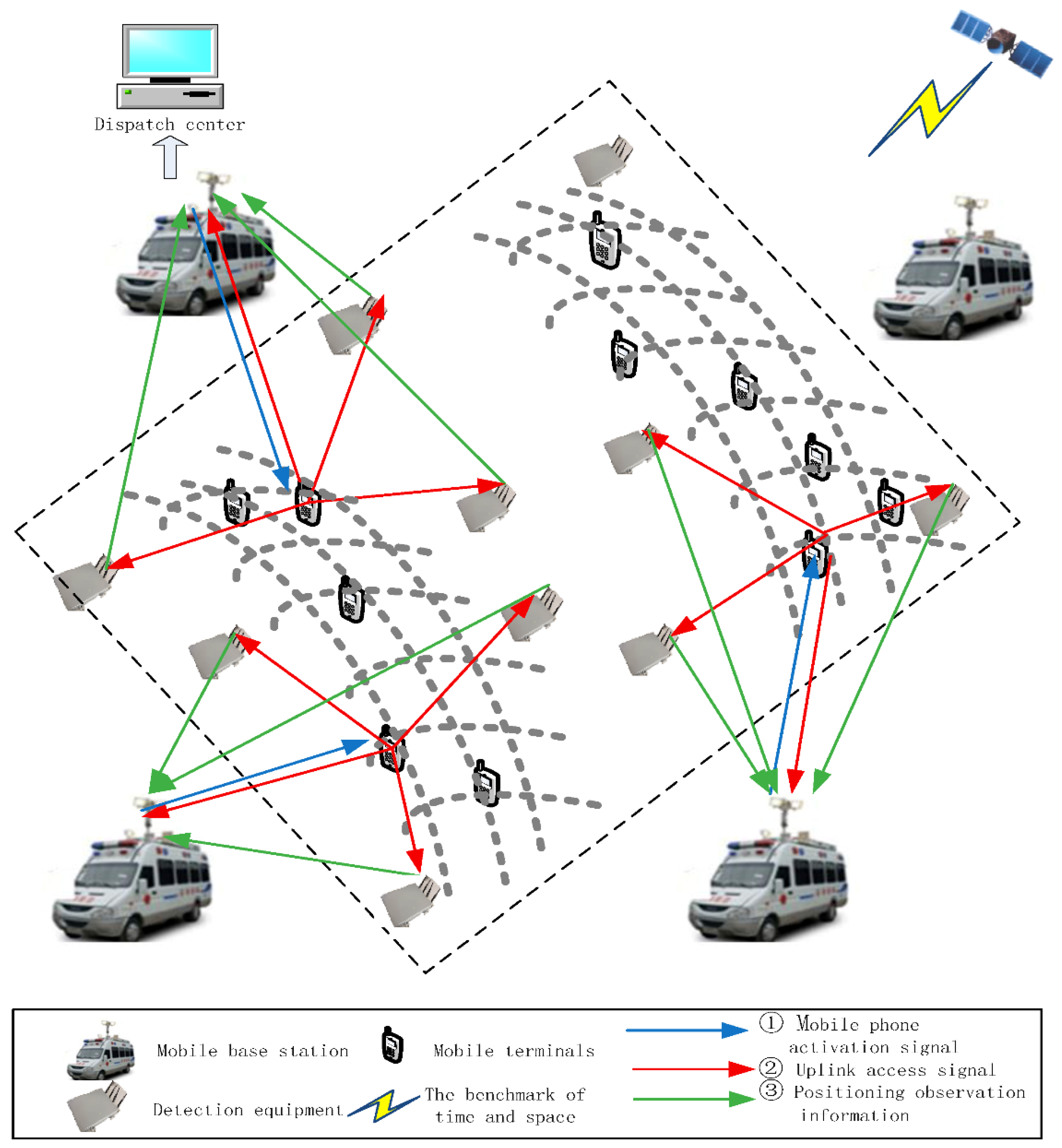
Based on the theoretical study of the mobile communication network and the location technology and algorithm, a wireless location system for the post-disaster complex environment was constructed. On the premise of not changing the existing mobile terminal, the system simulates the existing base station function and stimulates the mobile phone to transmit an access signal by broadcasting the paging signal, the access signal is captured by the detection equipment for TOA (time of arrival) estimation, and the system completes the ranging and uses the passive positioning algorithm to solve the localization. The basic structure of the system consists of one piece of master detection equipment and three pieces of slave detection equipment, which are designed to achieve three-dimensional positioning by using TDOA (time difference of arrival). To achieve higher accuracy when covering a larger area, you should increase the number of pieces of detection equipment in the system.

The function of the master detection device (mobile base station) is more complex. In addition to stimulating the user terminal to send access signals, it also serves as the synchronization source of the detection device and receives the ranging information from the detection device for positioning. The slave detection device only receives the access signal from the user terminal and sends the ranging information to the master detection equipment. Therefore, to achieve wireless positioning of a post-disaster complex environment in a large range and to solve the problem of weak signal acquisition difficulty due to signal attenuation and non-line-of-sight propagation, a positioning system with multiple pieces of detection equipment was built. The system consisted of a small number of pieces of main detection equipment with complex functions and more portable slave detection equipment. The architecture of a post-disaster search-and-rescue positioning system based on mobile communication is shown in Figure 1. The gray, dashed lines in Figure 1 are a simulated post-earthquake ruins’ environment.

After the disaster, the base station around the trapped people may not work properly. Additionally, the mobile terminal is looking for the base station. The main detection device sends the link control signal to the analog base station and the control mobile device sends the location update signal for registration. When the base station in the area is running normally, the master detection equipment sends control signals to inform the mobile terminal of the update of location information and the update of standby registration information. The specific positioning implementation process is as follows:

1. The master detection equipment sends the analog base station forward link control signal (paging signal) to control the mobile terminal receiving the signal to update its position, so as to send the position update signal for registration, and the mobile terminal sends the uplink access request signal.

2. The master detection equipment and the secondary detection equipment synchronously capture the uplink signal of the mobile terminal, obtain the arrival time, arrival angle, and arrival signal intensity of the terminal registration signal through several detection devices, and complete the positioning by combining with the location information of the mobile terminal.

3. Usually trapped people will carry mobile terminals; so, the location of trapped people can be known according to the location of mobile terminals, and the positioning results will be transmitted to the post-disaster rescue command center. Then, rescue teams will search and rescue according to the positioning results.

4. Portable detection equipment can be brought into the site of the post-disaster ruins by search-and-rescue teams to conduct close-range positioning and on-site search and rescue according to the positioning results.

To improve positioning efficiency and reduce information redundancy, it is hoped that the measurement information used in the positioning solution can be optimized. For example, the TDOA positioning solution requires a joint solution of multiple nodes, and the solution results of different node combinations are different. To obtain the optimal solution results, we want to select the optimal combination from redundant detection equipment to participate in the solution.

2.2. The Principle of Optimized Node Selection Algorithm and the Algorithm Flow

2.2.1. Principle of Optimal Selection Algorithm

The problem of node selection in a wireless positioning system is similar to that of sensor selection in a wireless sensor network. This kind of selection problem is usually expressed as an optimization problem for performance measurement. Its mathematical concept is expressed as

$$\underset{\gamma \in {\left\{0,1\right\}}^N}{\arg \min }f\left(E\left(\gamma \right)\right)\begin{array}{ccc}& \mathrm{s}.\mathrm{t}.& 1_N^T\gamma =L\end{array}$$

(1)

where $\gamma$ is a selection vector of length N and a scalar cost function $f\left(E\left(\gamma \right)\right)$ associated with the error covariance matrix $E$. The error covariance matrix is optimized to select the optimal subset with $L$ sensors from the $N$ sensors available. There are different cost functions, $f\left(E\left(\gamma \right)\right)$, to be used, and the typical choices minimize the sum of the eigenvalues of the matrix [23]:

$$f\left(E\left(\gamma \right)\right):=tr\left\{E\left(\gamma \right)\right\}$$

(2)

Equation (1) is a combinatorial optimization problem involving a search of $C_N^L$, which is obviously difficult to deal with, even on a small scale. In order to simplify the problem, some researchers relax the non-convex Boolean constraints $\gamma \in {\left\{0,1\right\}}^N$ into convex box constraints $\gamma \in {\left[0,1\right]}^N$ [24].

The general form of a non-linear measurement model can be expressed as

$$y_k=h_k(\psi ,{\omega }_k),k=1,2,\cdots ,N$$

(3)

where $y_k$ is the space or time measurement value of the first sensor, $\psi \in {ℝ}^N$ is the unknown parameter, and ${\omega }_k$ is the noise process, where $k=1,2,\cdots ,N$, $h_k$ is generally a non-linear equation; $y={\left[y_1,y_2,\cdots ,y_N\right]}^T\in {ℝ}^N$ is a collection of measurements. The probability density function (PDF) $p\left(y;\psi \right)$ of the measured values $y$ is parameterized by unknown vectors $\psi$.

These are the following assumptions:

Assumption 1.

Regular conditions: logarithmic likelihood values of measured values meet regular conditions$\mathbb{E}\left\{\frac{\partial \ln p(y;\psi )}{\partial \psi }\right\}=0$, which is the condition for the existence of CRB.

Assumption 2.

Independent measurement:$y_k$is an independent random variable sequence when$k=1,2,\cdots ,N$. As long as the above two assumptions are true, the proposed sensor selection framework is valid. If Assumption 1 is true, then the covariance of any unbiased estimator of unknown parameters$\widehat{\psi }\in {ℝ}^N$satisfies the famous in equation [25]

$$\mathbb{E}\left\{(\psi -\widehat{\psi }){(\psi -\widehat{\psi })}^T\right\}\ge C(\psi )=F^{-1}(\psi )$$

(4)

where$C(\psi )$is CRB matrix,$F\left(\psi \right)$is Fisher information matrix (FIM), and$F\left(\psi \right)$is given by the following equation

$$\begin{array}{c}F(\psi )=-\mathbb{E}\left\{\frac{{\partial }^2}{\partial \psi }{\left(\frac{\ln p(y;\psi )}{\partial \psi }\right)}^T\right\}\\ =\mathbb{E}\left\{\left(\frac{\partial \ln p(y;\psi )}{\partial \psi }\right){\left(\frac{\partial \ln p(y;\psi )}{\partial \psi }\right)}^T\right\}\in {ℝ}^{N\times N}\end{array}.$$

(5)

2.2.2. Process of Optimal Selection of Nodes Based on AOA and TDOA Hybrid Positioning

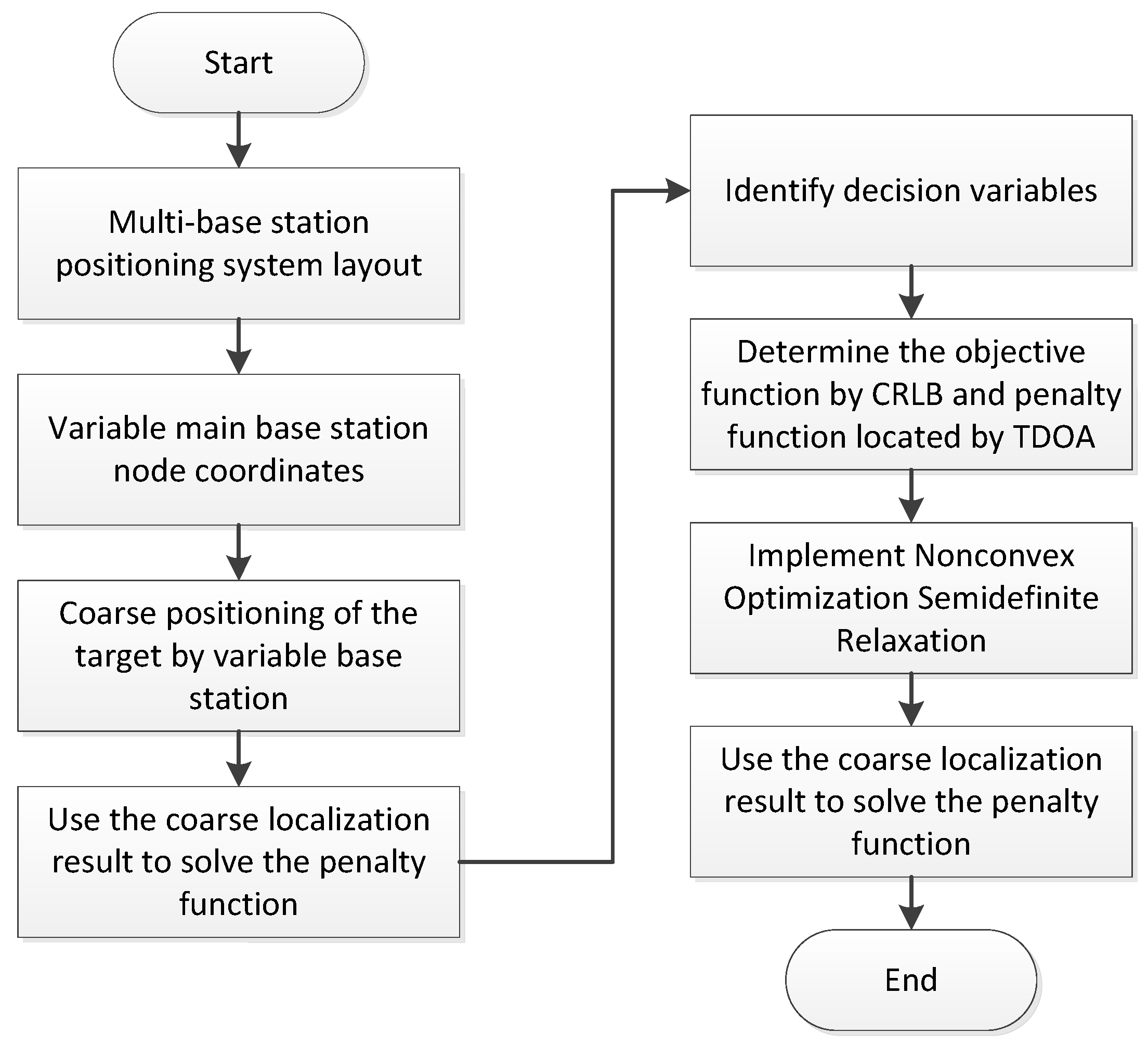
Node selection based on a mixed location of time difference of arrival (TDOA) and angle of arrival (AOA) can be achieved by minimizing the Cramer–Rao lower bound. CRLB is more complicated when the noise variance of different node distance measurements varies with different ruins. Using semi-determinate relaxation (SDR) with the most advanced node selection methods may lead to an incorrect node selection due to the ambiguity arising from relaxation. In this paper, a node selection method based on TDOA and AOA passive positioning is proposed; this explicitly combines the angle and distance information between the node and the user terminal to solve the fuzzy problem caused by SDR. Specifically, the problem of node selection with a known number of nodes was studied and expressed as a non-convex optimization problem. Then the non-convex problem was relaxed into convex semi-definite programming by SDR. A special vector was introduced to distinguish the reference nodes (mobile base stations) from the non-reference nodes (detection devices). Then, a non-convex optimization problem was expressed by using a Boolean vector as an optimization variable. Figure 2 shows the algorithm optimization process.

3. Optimization Selection Method of Location Detection Equipment Based on SDP

Based on the complexity and anisotropy of the channel in the ruin environment, the simple and direct method to achieve a more accurate positioning is to distribute more detection devices in the positioning area. However, the 3D TDOA and AOA fusion positioning algorithm needs to calculate the distance parameters of four nodes, which required us to select the optimal four nodes from multiple detection equipment for a positioning solution. For multi-detection equipment positioning system, TDOA and AOA are combined to improve positioning accuracy. As the TDOA algorithm needs to set a reference node to obtain the time difference, there must be one reference node in each group of solutions; its position affects the effect of the positioning precision. To adapt in a wide-area location and reduce the cost, the research team put forward a positioning system, which is shown in Figure 1. Here, the master node was designed as a variable mobile base station. It can participate in positioning as either the master node or the slave node.

The optimization process of the node selection in this word was divided into two stages. In the first stage, the target was roughly located and the main node was selected according to the results of rough location. In the second stage, when the primary node was determined, the remaining nodes (including other variable nodes) were optimized. The positioning equation, optimization principle, and process involved in the two stages are described in detail below.

3.1. TDOA and AOA Measurement Models and Performance

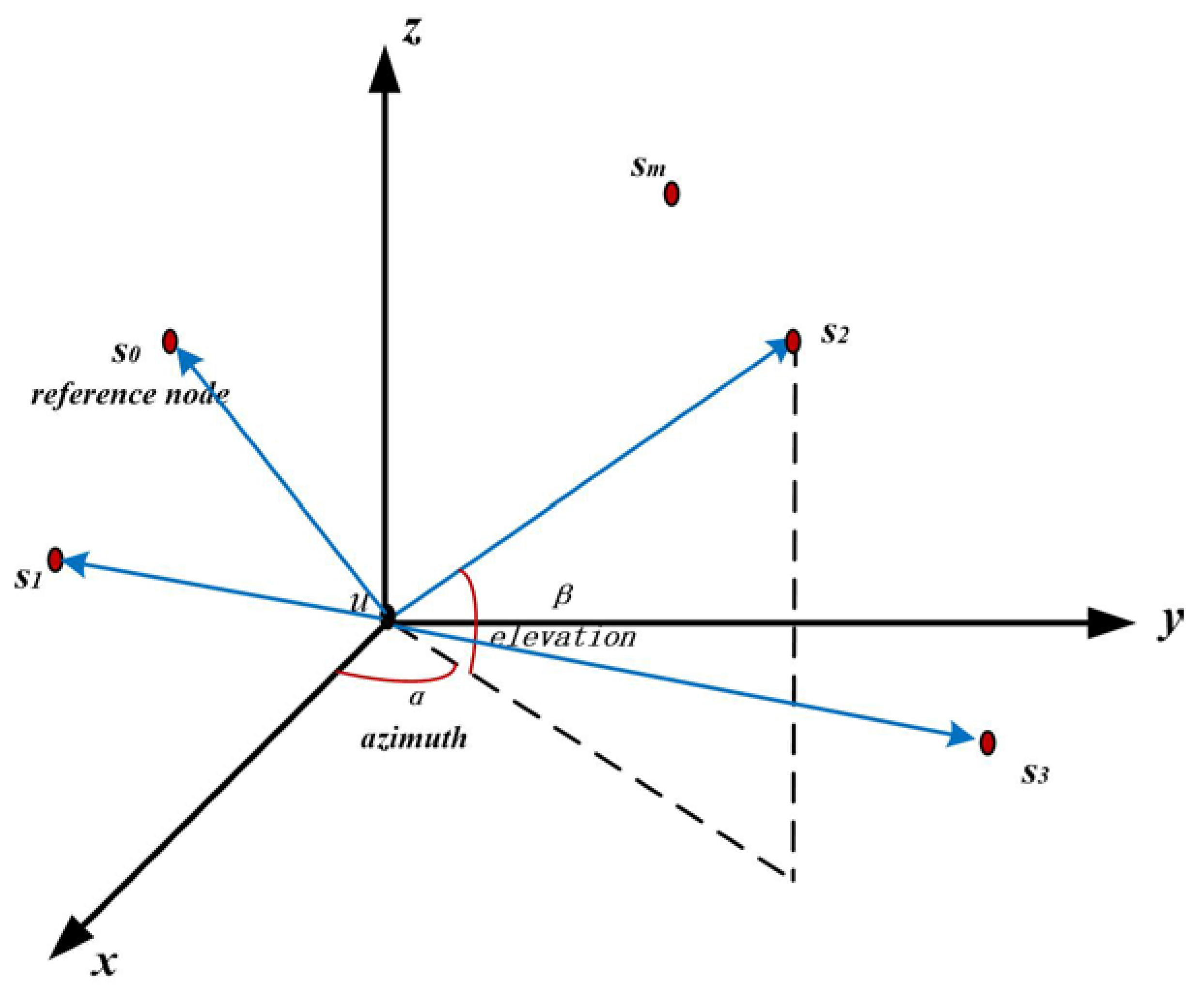
A passive location system is usually composed of the main mobile base stations and more from the mobile base stations. The main mobile base station radio induction signal is positioned in the access channel after a target is received. The induction signal sends an access request signal. The master–slave mobile base station positioning calculating variable is obtained by the capture of access. The positioning solution is the coordinates of the target.

Figure 3 is the schematic diagram of a TDOA and AOA 3D passive positioning model. The signal source has a set of azimuth and elevation angles relative to each sensor node.

Here we define:

• The coordinate vector of the main mobile base station is ${\mathit{s}}_0={[x_0,y_0,z_0]}^T$;
• The coordinate vectors of the slave stations are ${\mathit{s}}_i={[x_i,y_i,z_i]}^T\begin{array}{cc},& i=1,2,\cdots N\end{array}$;
• The target coordinate vector is $\mathit{u}={[x_t,y_t,z_t]}^T$;
• The distance between the target and mobile base station is $d_i$;
• The distance difference between the located target and the main station and from the slave station is $d_{0i}$;
• The speed of light is $c=0.3\hspace{0.17em}\mathrm{m}/\mathrm{ns}$;
• The elevation is $\beta$;
• The azimuth angle is $\alpha$.

3.1.1. AOA Measurement Model

The AOA method measures the arrival direction of the received signal based on the azimuth and elevation from the target to the receiver and gives azimuth ${\alpha }_i$ and elevation ${\beta }_i$ of the $i\mathrm{th}$ receiver, respectively.

$${\alpha }_i={\tan }^{-1}(\frac{y-y_i}{x-x_i})$$

(6)

$${\beta }_i={\tan }^{-1}(\frac{z-z_i}{\left(x-x_i\right)\cos {\alpha }_i+\left(y-y_i\right)\sin {\alpha }_i})$$

(7)

By using a trigonometric formula, Equations (6) and (7) can be sorted out, respectively:

$$\begin{array}{c}x\sin {\alpha }_i-y\cos {\alpha }_i=x_i\sin {\alpha }_i-y\cos {\alpha }_i\end{array}$$

(8)

$$x\sin {\beta }_i\cos {\alpha }_i-y\sin {\beta }_i\sin {\alpha }_i-z\cos {\beta }_i=x_i\sin {\beta }_i\cos {\alpha }_i+y_i\sin {\beta }_i\sin {\alpha }_i-z_i\cos {\beta }_i$$

(9)

To make it easier to deal with, rewrite these two things in this matrix form

$${\mathit{A}}_{A,i}{\mathit{x}}_1={\mathit{b}}_{A,i}\begin{array}{cc},& i=1,2,\cdots ,N\end{array}$$

(10)

where

$$\begin{gathered} {\mathit{b}}_{A,i}=\left[\begin{array}{c}{x}_i\sin {\alpha }_i-y_i\cos {\alpha }_i\\ x_i\sin {\beta }_i\cos {\alpha }_i+y_i\sin {\beta }_i\sin {\alpha }_i-z_i\cos {\beta }_i\end{array}\right] \\ {\mathit{A}}_{A,i}=\begin{array}{ll}[\begin{array}{lll}\sin {\alpha }_i& -\cos {\alpha }_i& 0\\ \sin {\beta }_i\cos {\alpha }_i& \sin {\beta }_i\sin {\alpha }_i& -\cos {\beta }_i\end{array}& O_{2\times N}\end{array}] \end{gathered}$$

(11)

When Equation (11) is extended to all receiving base stations, the final AOA equation is expressed as follows

$${\mathit{A}}_A{\mathit{x}}_1={\mathit{b}}_A$$

(12)

where

$$\begin{array}{l}{\mathit{b}}_A={\left[b_{A,1}^T\begin{array}{cc}\cdots & b_{A,N}^T\end{array}\right]}^T\\ {\mathit{A}}_A={\left[\begin{array}{ccc}{A}_{A,1}^T& \cdots & A_{A,N}^T\end{array}\right]}^T\end{array}$$

(13)

The relationship among the actual measured azimuth, elevation, target position coordinates, and the real value is expressed as

$$\widehat{\mathsf{\alpha }}=\mathsf{\alpha }+{\mathsf{\omega }}_{\alpha },\widehat{\mathsf{\beta }}=\mathsf{\beta }+{\mathsf{\omega }}_{\beta },{\widehat{s}}_t=s_t+\Delta s$$

(14)

The AOA measurement error vector is expressed as ${\mathsf{\omega }}_A={\left[\begin{array}{ccc}{\mathsf{\omega }}_{A,1}^T& \cdots & {\mathsf{\omega }}_{A,N}^T\end{array}\right]}^T$, where ${\mathsf{\omega }}_{A,i}^T={\left[\begin{array}{cc}\Delta {\alpha }_i& \Delta {\beta }_i\end{array}\right]}^T$. It can also be written as the azimuth measurement noise and elevation measurement noise, respectively, expressed as

$$\begin{array}{l}{\mathsf{\omega }}_{\alpha }^T={\left[\begin{array}{cc}\Delta {\alpha }_1,\Delta {\alpha }_2,\cdots ,& \Delta {\alpha }_N\end{array}\right]}^T\\ {\mathsf{\omega }}_{\beta }^T={\left[\begin{array}{cc}\Delta {\beta }_1,\Delta {\beta }_2,\cdots ,& \Delta {\beta }_N\end{array}\right]}^T\end{array}$$

(15)

Here, it is considered that all noises are Gaussian noises with an average of 0 and the covariance matrices are, respectively, expressed as $Q_{{\omega }_{\alpha }}=\mathrm{E}[{\mathsf{\omega }}_{\alpha }{}^T{\mathsf{\omega }}_{\alpha }]$, $Q_{{\omega }_{\beta }}=\mathrm{E}[{\mathsf{\omega }}_{\beta }{}^T{\mathsf{\omega }}_{\beta }]$, $Q_{{\omega }_A}=diag\left\{Q_{{\mathsf{\omega }}_{\alpha }}{Q}_{{\mathsf{\omega }}_{\beta }}\right\}$. When the measurement noise is small, $\cos (\Delta {\alpha }_i)\approx 1,\sin \left(\Delta {\alpha }_i\right)=\Delta {\alpha }_i$, and the approximate value is obtained. The observed values of each parameter are substituted into Equations (8) and (9), ignoring the quadratic error term, and the equation with measurement noise is shown in the following formula

$$\begin{array}{l}\sin {\alpha }_i\left(x-x_i\right)-\cos {\alpha }_i\left(y-y_i\right)={\omega }_{{\alpha }_i}{d}_i\cos {\beta }_i^0{\omega }_{{\alpha }_i}\\ \sin {\beta }_i\cos {\epsilon }_i\left(x-x_i\right)+\sin {\beta }_i\sin {\alpha }_i\left(y-y_i\right)-\cos {\beta }_i\left(z-z_i\right)=d_i{\omega }_{{\beta }_i}\end{array}$$

(16)

The non-linear equations shown in Equation (16) are usually difficult to solve directly; so, they are transformed into matrices to facilitate solving. The weighted least square method is used to solve the equation.

$$\begin{array}{c}{\mathit{B}}^0{\mathsf{\omega }}_A\approx {\widehat{\mathit{b}}}_1-{\widehat{\mathit{A}}}_1{\widehat{\mathit{x}}}_t\end{array}$$

(17)

where

$$\begin{array}{c}\mathit{G}={\left[\begin{array}{cc}{\mathit{G}}_{\alpha }^T& {\mathit{G}}_{\beta }^T\end{array}\right]}^T\\ {\mathit{G}}_{\alpha }={\left[\begin{array}{cccc}{\mathit{g}}_{\alpha 1}& {\mathit{g}}_{\alpha 2}& \cdots & {\mathit{g}}_{\alpha N}\end{array}\right]}^T\\ {\mathit{G}}_{\beta }={\left[\begin{array}{cccc}{\mathit{g}}_{\beta 1}& {\mathit{g}}_{\beta 2}& \cdots & {\mathit{g}}_{\beta N}\end{array}\right]}^T\\ {\mathit{B}}^0=\left[\begin{array}{cc}{\mathit{B}}_{\alpha }^0& 0\\ 0& {\mathit{B}}_{\beta }^0\end{array}\right]\end{array}$$

where

$$\begin{array}{c}{\mathrm{B}}_{\alpha }^0=diag\left(\left[{\mathrm{d}}_1^{}\cos {\beta }_1^{},{\mathrm{d}}_2^{}\cos {\beta }_2^{},\dots ,{\mathrm{d}}_N^{}\cos {\beta }_N^{}\right]\right)\\ {\mathrm{B}}_{\beta }^0=diag\left(\left[{\mathrm{d}}_1^{},{\mathrm{d}}_2^{},\dots ,{\mathrm{d}}_N^{}\right]\right)\\ {\mathbf{g}}_{\alpha i}={\left[-\sin {\alpha }_{i,}\cos {\alpha }_i,0\right]}^{\mathrm{T}},i=1,2\dots ,N\\ {\mathbf{g}}_{\beta i}={\left[-\sin {\beta }_i\cos {\beta }_{i,},-\sin {\beta }_i\sin {\beta }_{i,},\cos {\beta }_i\right]}^{\mathrm{T}}\end{array}$$

Let the weighting matrix be $W=E{\left[B^0{\omega }_A{\omega }_A{}^T{B}^{0T}\right]}^{-1}={\left(B^{0}Q{B}^{0T}\right)}^{-1}$. Then, the objective function can be defined as

$$J(s_t)={({\widehat{b}}_{\mathbf{1}}-G{s}_t)}^{T}W({\widehat{b}}_{\mathbf{1}}-G{s}_t)$$

(18)

Applying the weighted least squares optimization to solve the above equation, we can get the following formula.

$$s_t={\left(G^{T}WG\right)}^{-1}{G}^{T}Wh$$

(19)

where

$$\mathit{h}={\left[\begin{array}{cc}{\mathbf{1}}^T{\left({\mathit{G}}_{\alpha }\odot \mathit{S}\right)}^T& {\mathbf{1}}^T{\left({\mathit{G}}_{\alpha }\odot \mathit{S}\right)}^T\end{array}\right]}^T$$

The advantages of the AOA-based positioning method are the simple positioning system composition and fast positioning speed. The optimization algorithm of the location detection equipment selection was proposed in this section, the coarse location of the target was realized, and the location result was applied to the reference node selection.

3.1.2. TDOA Measurement Model

The TDOA measurement using the signal propagation velocity (light speed) multiplied by the propagation time is converted to the distance difference. The distance of each pair is obtained by adding the distance difference measured at the receiving end to the visual distance of the corresponding sender and receiver. In fact, there is a linear relationship between the TDOA measurements and the distance between the receiver and sender. For the positioning system shown in Figure 3, the master node S0 serves as the receiving and transmitting node; the distance between it and the slave node can be calculated by the following formula [26]:

$$d_{0,i}=d_0-d_i=c\cdot t_i$$

(20)

where $d_{0,i}$ is the difference in distance between the target and master node and the slave node $i$ (R-TDOA). The $\Delta t_i$ is arrival time difference (TDOA). The calculation formula of $d_0$, $d_i$ is as follows:

$$d_0={\mathit{s}}_0-{\mathit{s}}_t$$

(21)

$$d_i={\mathit{s}}_i-{\mathit{s}}_t$$

(22)

It can be obtained from Equation (14)

$$d_{0,i}+d_i=d_0$$

(23)

Substitute Equations (21) and (22) into Equation (23), square both sides of the equation, and derive

$$\left({\mathit{s}}_i^T-{\mathit{s}}_0^T\right){\mathit{s}}_t-d_{0,i}{d}_i=\frac{1}{2}\left(d_{0,i}^2+{\mathit{s}}_i^T{\mathit{s}}_i-{\mathit{s}}_0^T{\mathit{s}}_0\right)$$

(24)

The operation of Formulas (4)–(7) on all slave nodes gives the matrix-form equation

$${\mathit{A}}_T{\mathit{x}}_1={\mathit{b}}_T$$

(25)

where

$$\begin{array}{l}{\mathit{b}}_T={\left[b_{T,1}^T\begin{array}{cc}\cdots & b_{T,N}^T\end{array}\right]}^T\\ \left[b_{T,i}^T\right]=\frac{1}{2}\left(d_{0,i}^2+s_i^T{s}_i-s_0^T{s}_0\right)\\ {\mathit{A}}_T={\left[\begin{array}{ccc}{A}_{T,1}^T& \cdots & A_{T,N}^T\end{array}\right]}^T\\ A_{T,i}(1,:)=\left[\begin{array}{cc}{s}_i^T-s_0^T& e_i^T\otimes d_{0,i}\end{array}\right]\\ {\mathit{x}}_1={\left[\begin{array}{cc}{\mathit{s}}_t^T& {\mathit{d}}^T\end{array}\right]}^T\\ \mathit{d}={\left[\begin{array}{ccc}{d}_1& \cdots & d_N\end{array}\right]}^T\end{array}$$

Consider a D-dimensional (D = 2 or 3) multi-node positioning system, which consists of N nodes with known positions and a user terminal with unknown positions. Here, it is assumed that the R-TDOA distance measurement noise ${\omega }_{Ti},i=1,2,\cdots ,N$ between each detection device and the user terminal is independent of each other and all follow the Gaussian distribution of zero mean and zero variance.

Rewrite Equation (25) as follows

$$\begin{array}{c}0={\mathit{b}}_T-{\mathit{A}}_T{\mathit{x}}_1\end{array}$$

(26)

After considering the influence of R-TDOA measurement noise, the left side of Equation (26) is not 0, and the 0 expression is regarded as an error vector. In other words, replace the noisy measurements in Equation (26) to obtain the error vector, the difference between the two terms on the right. This can be represented as a vector:

$$\begin{array}{c}{\mathsf{\omega }}_T={\widehat{\mathit{b}}}_T-{\widehat{\mathit{A}}}_T{\mathit{x}}_1\end{array}$$

(27)

where ${\mathsf{\omega }}_T$ is the measurement error vector of the R-TDOA distance. The WLS solution of Equation (27) is to obtain the minimum unknown value of the cost function, i.e.,

$$\begin{array}{c}{\widehat{\mathit{x}}}_1={\left({\widehat{\mathit{A}}}_T^{\mathrm{T}}{\mathit{W}}_T{\widehat{\mathit{A}}}_T\right)}^{-1}{\widehat{\mathit{A}}}_T^{\mathrm{T}}{\mathit{W}}_T{\widehat{\mathit{b}}}_T\end{array}$$

(28)

The measurement error of the R-TDOA range can be expressed as follows:

$$\mathit{d}=\widehat{\mathit{d}}-{\mathsf{\omega }}_T$$

(29)

where $\widehat{d}$ is the measured value, $d$ is the correct value, and $d=\left[\begin{array}{ccc}{d}_1^T& \cdots & d_N^T\end{array}\right]$ contains all noiseless measurements. The distance measurement error vector is expressed as ${\mathsf{\omega }}_T={\left[\begin{array}{ccc}{\omega }_{T,1}^T& \cdots & {\omega }_{T,N}^T\end{array}\right]}^T$.

Calculate the error covariance matrix:

$$\begin{array}{l}{\mathit{C}}_{\omega T}=E\left[{\mathsf{\omega }}_T{\mathsf{\omega }}_T^T\right]=diag\left(C_{\mathsf{\omega }T,i}\right)\\ {\mathit{C}}_{\omega T,i}=E\left[{\mathsf{\omega }}_{T,i}{\mathsf{\omega }}_{T,i}^T\right]\begin{array}{cc},& i=1,2\cdots N\end{array}\end{array}$$

(30)

The variance of the estimated parameters is minimized by considering the inverse of the error covariance matrix as the weighted matrix. The result is:

$$\begin{array}{c}{W}_1=C_{{\omega }_T}^{-1}\end{array}$$

(31)

Formula (31) is replaced by $W_1$. Under the given assumptions, Formula (28) derives the approximate maximum likelihood value. The error vector ${\mathsf{\omega }}_1$ is a normal random distribution vector with a mean of 0. Represent ${\widehat{\mathit{x}}}_1$, ${\widehat{\mathit{b}}}_T$, and ${\widehat{\mathit{A}}}_T$, respectively, as ${\mathit{x}}_1+\Delta {\mathit{x}}_1$, ${\mathit{b}}_T+\Delta {\mathit{b}}_T$, and ${\mathit{A}}_T+\Delta {\mathit{A}}_T$. Then, substitute them into Equation (28).

$$\begin{array}{c}\begin{array}{c}\left({\mathit{A}}_T^{\mathrm{T}}+\Delta {\mathit{A}}_T^{\mathrm{T}}\right){\mathit{W}}_1\left({\mathit{A}}_T+\Delta {\mathit{A}}_T\right)\left({\mathit{x}}_1+\Delta {\mathit{x}}_1\right)\\ =\left({\mathit{A}}_T^T+\Delta {\mathit{A}}_T^T\right){\mathit{W}}_1\left({\mathit{b}}_T+\Delta {\mathit{b}}_T\right)\end{array}\end{array}$$

(32)

By eliminating the error terms of the second order and above, only the linear terms are retained, which can be obtained by Equation (27).

$$\begin{array}{c}\Delta {\mathit{x}}_1={\left({\mathit{A}}_T^{\mathrm{T}}{\mathit{W}}_1{\mathit{A}}_T\right)}^{-1}{\mathit{A}}_T^{\mathrm{T}}{\mathit{W}}_1{\mathsf{\omega }}_T\end{array}$$

(33)

Multiply Equation (28) by its transpose, take the expectation, and the covariance matrix of ${\widehat{\mathit{x}}}_1$ is:

$$\begin{array}{c}\mathrm{cov}\left({\widehat{\mathit{x}}}_1\right)={\left({\mathit{A}}_T^{\mathrm{T}}{\mathit{W}}_1{\mathit{A}}_T\right)}^{-1}\end{array}$$

(34)

3.1.3. Positioning Performance Analysis of TDOA

In the positioning system, random measurement error inevitably leads to the error of the target positioning results. Commonly, we use root mean square error (RMSE) and CRLB for the accuracy of the positioning results [27]. RMSE is the square root of the mean square error. The CRLB is the lower bound of the variance of the unbiased estimator; it is an important index to evaluate the accuracy of the unbiased estimator. In this paper, root mean square error (RMSE) and CRLB are used to measure the positioning accuracy.

RMSE can be calculated by a Monte Carlo experiment:

$$RSME=\sqrt{\frac{{\displaystyle \sum _{i=1}^T{\Vert {\widehat{\mathit{x}}}_1{}^{\left(i\right)}-s_t\Vert }_2^2}}{T}}$$

(35)

where T is the number of tests. Theoretically, when the number of tests is infinite, the value of RMSE is approximate to the square root of the trace of the covariance matrix.

$$CRL{B}_{\mathrm{tdoa}}\left(s_t\right)=I^{-1}\left({\mathit{s}}_t\right)={\left[{\left(\frac{\partial \mathit{q}}{\partial {\mathit{s}}_t}\right)}^T{\mathit{C}}_{\omega T}^{-1}\frac{\partial \mathit{q}}{\partial {\mathit{s}}_t}\right]}^{-1}={\left[{\left(\frac{\partial \mathit{d}}{\partial {\mathit{s}}_t}\right)}^T{\mathit{C}}_{\omega T}^{-1}\frac{\partial \mathit{d}}{\partial {\mathit{s}}_t}\right]}^{-1}$$

(36)

where $p(\widehat{q};x_t)$ represents the probability density function of $\widehat{q}$, which, parameterized by unknown variables $s_t$, and $\widehat{q}$, is the vector with noise measurements.

Assuming that

$$\begin{array}{l}\frac{\partial \mathit{d}}{\partial {\mathit{s}}_t}={\left[\begin{array}{ccc}{\left(\frac{\partial {\mathit{d}}_1}{\partial {\mathit{s}}_t}\right)}^T& \cdots & {\left(\frac{\partial {\mathit{d}}_N}{\partial {\mathit{s}}_t}\right)}^T\end{array}\right]}^T=\mathit{H}\\ \frac{\partial {\mathit{d}}_i}{\partial {\mathit{s}}_t}=\left[\frac{{\left({\mathit{s}}_t-{\mathit{s}}_0\right)}^T}{{\mathit{s}}_t-{\mathit{s}}_0}-\frac{{\left({\mathit{s}}_t-{\mathit{s}}_i\right)}^T}{{\mathit{s}}_t-{\mathit{s}}_i}\right]\begin{array}{cc}={\mathit{H}}_i,& i=1\cdots N\end{array}\end{array}$$

(37)

Then,

$$CRL{B}_{\mathrm{tdoa}}\left(s_t\right)={\left({\mathit{H}}^T{\mathit{Q}}^{-1}\mathit{H}\right)}^{-1}$$

(38)

The CRLB of the WLS location estimation algorithm is the objective function of the detection device selection. In this paper, the TDOA-based approximate optimal detection device nodes were used for wireless terminal positioning. The decision variables and optimization problem construction process are given below.

3.2. Optimal Decision Variable Design

The purpose of the location node selection algorithm is to select $L$ nodes from $N$ nodes to participate in positioning, so that the selected $L$ nodes can obtain the optimal positioning accuracy. Node selection is how to represent the location accuracy provided by the nodal point set. For 3D TDOA positioning, only four detection devices, one master and three slaves, are required. We must determine the way to select the best four nodes to solve the position from the multi-detection equipment of the positioning system. When $N$ is large, this kind of large-scale selection problem is very complicated to calculate. A Boolean vector $\mathsf{\beta }$ is usually defined to determine whether each node is selected. $\mathsf{\beta }$ defined as

$$\begin{array}{c}\mathsf{\beta }={\left[{\beta }_1,{\beta }_2,\cdots ,{\beta }_N\right]}^T,{\beta }_i\in \left\{0,1\right\}\end{array}$$

(39)

If ${\beta }_i$ equals 1, the $i\mathrm{th}$ slave node will be selected. If it equals 0, it is not selected.

For the post-disaster wireless location system, the fixed reference node is not the optimal choice for the remote location target. In order to improve positioning accuracy, this section sets multiple variable nodes (optional as a reference node, optional as a slave node, optional as not selected) [12]. Then, we must change the Boolean vector $\mathsf{\beta }$.

$$\begin{array}{c}\mathsf{\beta }={\left[{\beta }_1,\cdots ,{\beta }_M,{\beta }_{M+1},\cdots ,{\beta }_N\right]}^T\end{array}$$

(40)

where $\{\begin{array}{l}{\beta }_i\in \left\{0,1,-1\right\},1\le i\le M\\ {\beta }_i\in \left\{0,1\right\},M+1\le i\le N\end{array}$. If ${\beta }_i$ equals 1, the $i\mathrm{th}$ slave node will be selected. If it equals 0, it is not selected. If it is −1, it is selected as the reference node. It can be summarized as a constraint condition. The first M nodes are variable nodes, and it is accordingly assumed that these nodes have a fixed position coordinate.

Construct a $N\times \left(L-1\right)$ matrix using Equation (40), which is the sub-matrix of $diag(\mathsf{\omega })$, by setting all the elements of the row corresponding to the reference node to −1 and then deleting all the columns corresponding to the reference node and unselected node, so $P$ satisfies the following equation:

$$\begin{array}{c}{P}^{T}P={\mathbf{I}}_{L-1}+{\mathbf{1}}_{L-1}{\mathbf{1}}_{L-1}^T\\ P{\left(P^{T}P\right)}^{-1}{P}^T=\frac{1}{L}\left(Ldiag(\mathsf{\beta })-\mathsf{\beta }{\mathsf{\beta }}^T\right)\end{array}$$

(41)

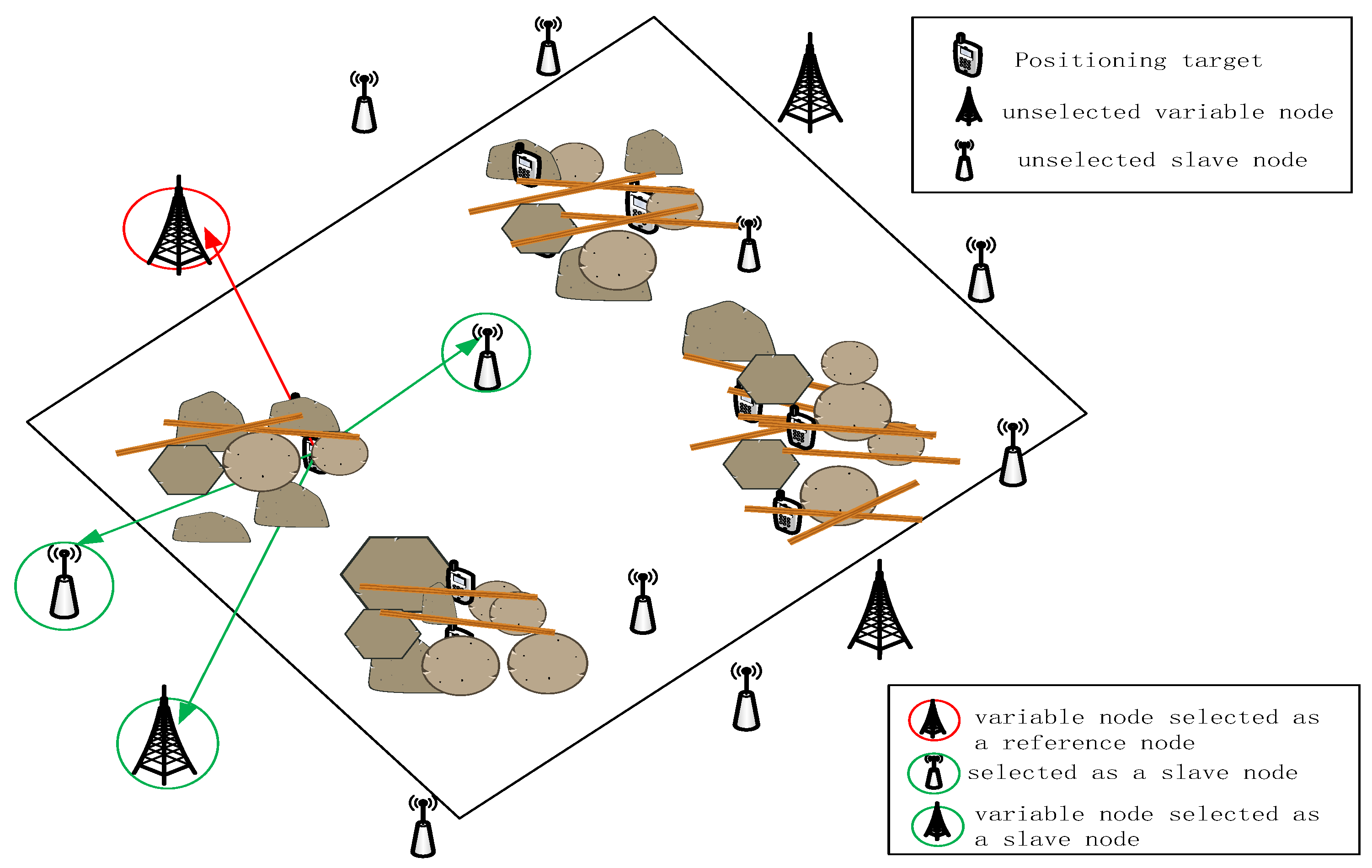
Figure 4 shows how to select a wireless location node after a disaster. The reference node (main mobile base station) in the positioning system has a processing center, which collects the measurement data and performs the positioning solver to estimate the user terminal location. In a post-disaster location system with multiple detection devices, it is impossible to locate all nodes. Therefore, you need to select nodes. Figure 4 shows the principle of primary and slave detection device selection in TDOA- and AOA-based positioning. According to certain criteria, the best node subset is selected from the positioning system to achieve the best positioning accuracy. Then, the source location method is used to locate the user terminal. Typically, the processing center performs node selection and terminal location. The ochre circles are simulated post-earthquake collapse sites.

3.3. Optimization Problem Construction and Relaxation Process

When one of $M$ variable nodes is selected as the reference node and $L-1$ of the remaining ($N-1$) nodes is selected as the slave node, there should be $L-1$ elements of the Boolean vector as “1”, which together with the reference nodes selected as the main detection device constitute all nodes. This is a typical selection optimization method, and the CRLB using the selected node positioning Formula (38) can be written in the following form:

$$CRL{B}_{\mathrm{tdoa}}^{}({\mathit{s}}_t)={\left({\mathit{H}}^T\mathbf{P}{\left({\mathbf{P}}^T\mathit{Q}\mathbf{P}\right)}^{-1}{\mathbf{P}}^T\mathit{H}\right)}^{-1}$$

(42)

Refer to Formula (37) for the specific form. According to Equation (42), the node selection problem can be expressed as the following optimization problem.

$$\begin{array}{ccc}\underset{\mathsf{\beta }}{min}& & \mathit{tr}\left\{{\left({\mathit{H}}^T\mathbf{P}{\left({\mathbf{P}}^T\mathit{Q}\mathbf{P}\right)}^{-1}{\mathbf{P}}^T\mathit{H}\right)}^1\right\}\\ & & \mathrm{s}.\mathrm{t}.{\mathbf{1}}_N^T\mathsf{\beta }=L\\ & & \mathsf{\beta }\in \{0,1{\}}^N\end{array}$$

(43)

For the method in this paper, the reference node was selected from the variable nodes and the best reference node was determined by rough position. This idea is reflected in the optimization algorithm by adding penalty terms to the original optimization selection problem [14], as shown in the following formula:

$$\begin{array}{ccc}\underset{\mathsf{\beta }}{\min }& & \mathit{tr}\{CRL{B}_{\mathrm{tdoa}}(\mathsf{\beta })\}+\lambda {\displaystyle \sum _{j=1}^N}{\beta }_j\frac{d_j}{{\displaystyle \sum _{j=1}^N}{d}_j}\\ & & \mathrm{s}.\mathrm{t}.{\mathbf{1}}_N^T\mathsf{\beta }=L\\ & & \mathsf{\beta }\in \{0,1{\}}^N\end{array}$$

(44)

where $d_j=\Vert {\mathit{s}}_t-{\mathit{s}}_j\Vert$ is the distance between the user terminal and the $j\mathrm{th}$ detection device and $\lambda$ is the penalty factor. In the post-disaster positioning, the value of $\lambda$ can be determined by the maximum station range and the total number of pieces of detection equipment. Simulation results showed that the performance of this method was insensitive to values, and values can be selected in a wide range. The coefficient $d_j/{\displaystyle \sum }_{j=1}^N{d}_j$ corresponds to ${\beta }_j$ and is related to $d_j$. Obviously, the smaller the value of $d_j$, the greater the probability that the $j\mathrm{th}$ device will be selected because this is a minimization problem. This makes sense because a weak signal from user terminals has a higher probability of transmitting signals that would be picked up by a closer detector; therefore, the closer detector would be preferred under the same CRLB conditions.

In the above equation, $tr\left\{CRL{B}_{\mathrm{tdoa}}^{}({\mathit{s}}_t)\right\}$, the objective function is non-convex relative to the decision variable, and SDR needs to be applied. A helper variable $W$ is introduced here.

$${\left({\left[\mathit{H},{\mathbf{1}}_N\right]}^{T}diag(\mathsf{\beta }){\mathit{Q}}^{-1}diag(\mathsf{\beta })\left[\mathit{H},{\mathbf{1}}_N\right]\right)}^{-1}\le \mathit{W}$$

(45)

By introducing $P=\mathsf{\beta }{\mathsf{\beta }}^T$ and using Schur’s complement theory, the following SDP problems can be obtained.

$$\begin{array}{}& \underset{\mathsf{\beta },\mathit{W},\mathbf{P}}{\min }\mathit{tr}\{\mathit{W}\}+d(\mathsf{\beta })\left(46\mathrm{a}\right)& \mathrm{s}.\mathrm{t}.\left[\begin{array}{cc}W& \mathbf{I}\\ \mathit{I}& {[\mathit{H},{\mathbf{1}}_N]}^T\mathit{diag}(\mathsf{\beta }){\mathit{Q}}^{-1}\mathit{diag}(\mathsf{\beta })[\mathit{H},{\mathbf{1}}_N]\end{array}\right]\ge 0\left(46\mathrm{b}\right)& \left[\begin{array}{cc}\mathbf{P}& \mathsf{\beta }\\ {\mathsf{\beta }}^T& 1\end{array}\right]\ge 0\left(46\mathrm{c}\right)& \mathit{Diag}(\mathbf{P})=\mathsf{\beta }\left(46\mathrm{d}\right)& \mathrm{tr}\left\{\mathbf{P}\right\}=L\end{array}$$

where $d(\mathsf{\beta })=\lambda {\displaystyle \sum _{j=1}^N}{\beta }_j·(d_j/\sum _{j=1}^N{d}_j)$ ; the rank of a non-convex constrained matrix is declined to $rank(P)=1$. It can be derived from Equations (46b) and (46c) that $0\le {\beta }_j^2\le P_{jj}={\beta }_j$, i.e., $0\le {\beta }_j\le 1$. The flag of the selected probe device node is determined by setting the $L$ maximum elements of the SDP solution to “1” and the remaining elements to “0”. After the above transformation, the objective function and constraint conditions in the optimization problem are transformed into convex functions about $\mathsf{\beta }$ and $W$, then the solution method can also be transformed into a convex optimization solution, which can be directly solved by using the CVX toolbox of MATLAB based on the interior point method.

As can be seen, the problem of selecting the reference detection device depends on the real target location, which is impossible. To solve this problem, a rough estimate of the location of the user terminal can be obtained by running a simple positioning method to select the variable probe device before making a reference probe device selection. In this paper, AOA is used for rough target positioning.

4. Simulation Results and Analysis

This section will give the performance analysis of the proposed SDP-based node selection algorithm. Compared with the performance of other node selection optimization algorithms, the shortest distance method (SDM) [28] directly selects the detection equipment closest to the signal source from all the nodes of the detection device; the exhaustive search method (ESM) [29] traverses all kinds of node combinations and selects the node with the lowest distance. The node combination for optimal positioning performance adopts the method of SDP optimization but fixing one main detection device (1st-SDP) [6]. The simulation results show the RMSE performance of different node selection algorithms when the R-TDOA measurement error intensity varies.

The simulation was carried out on a PC with a CPU of Intel(R) Core(TM) I5-8500K @ 3.00 GHz and 32 G memory. In the simulation, SDP was solved by the CVX toolbox of MATLAB. For this part, the performance of the proposed method was simulated and analyzed for the wide-area multi-detection device positioning network involved in this paper. Define a 1000 m × 1000 m area. Assume that 1000 positioning targets are randomly distributed in this area and 100 detection devices are distributed in this area. For the definition of the above positioning area, refer to [30] to optimize the layout of detection equipment.

4.1. Deployment of Variable Reference Detection Devices

The variable reference detection device has three functions in the optimized selection algorithm. On the one hand, it can realize the rough AOA location of the target, and the penalty function can be obtained from the distance between the target position and the main detection device. On the other hand, it is used as the reference main detection device in the optimized node selection algorithm based on TDOA. In addition, the variable probe device can also be used as a slave node. From the above analysis, the deployment of variable detection equipment is also important.

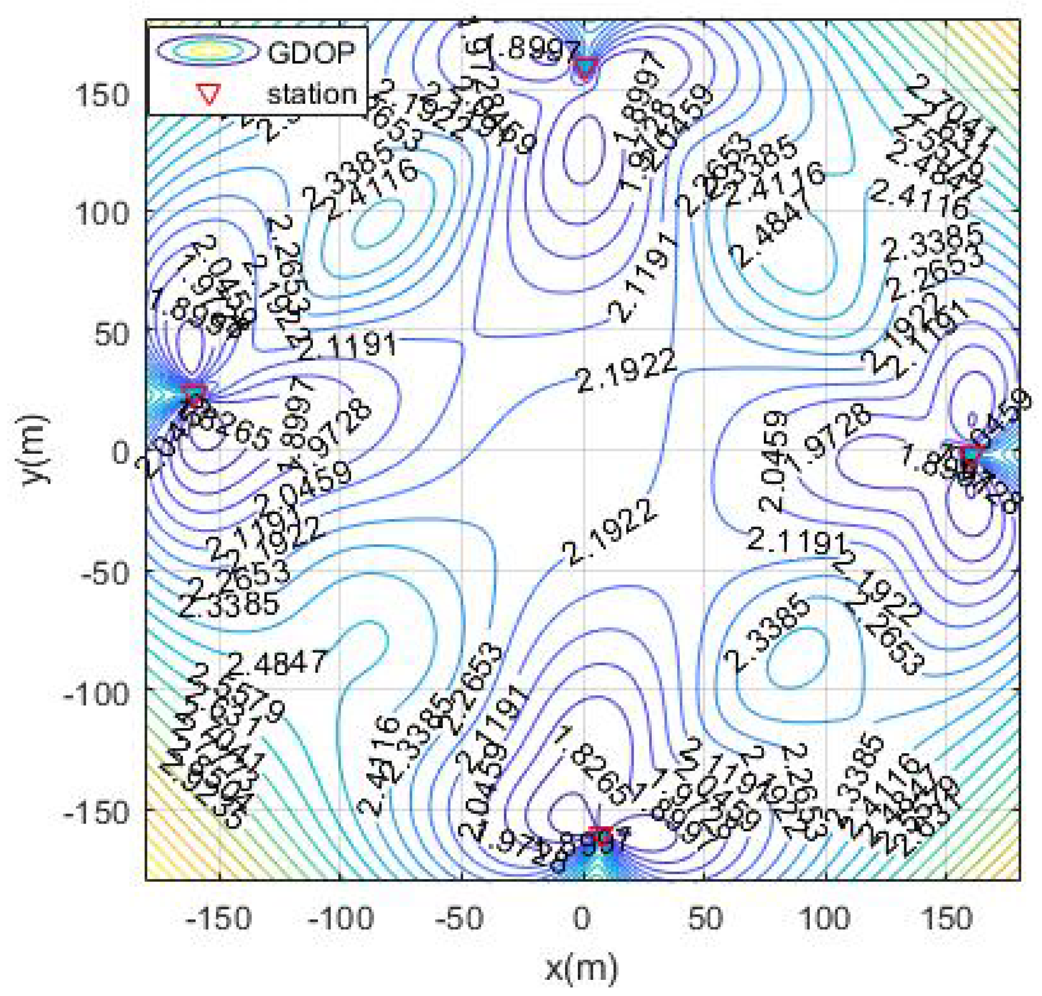
According to [30], the highest geometric accuracy of positioning is the case of the midpoint station on four sides, as shown in the Figure 5. Therefore, the deployment of the variable reference detection device was selected near the midpoint of the four sides of the region.

4.2. Influence Analysis of Penalty Factor on Optimization Node Selection Algorithm

The optimization algorithm designed for this chapter is an optimization problem with constraints: the independent variable cannot be arbitrarily selected, which leads to many unconstrained optimization algorithms that cannot be used. Compared with unconstrained optimization problems, this increases the complexity of the problem. If the penalty term transformed by a constraint is added to the objective function, it is transformed into the familiar unconstrained optimization problem. The value of the penalty factor must be greater than 0 and must be given before optimization.

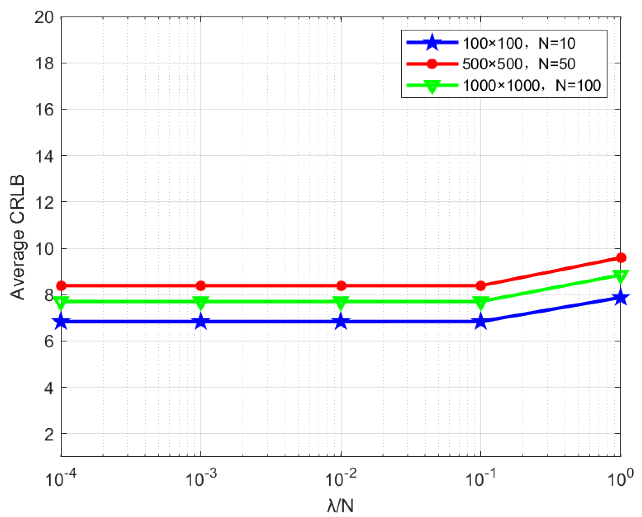
In practice, the value of a penalty factor can be determined by the size of the positioning scene and the total number of nodes. For post-disaster search-and-rescue wireless positioning, the location scene depends on the range of weak signals transmitted by user terminals that can be captured by detection devices. The sensitivity of the proposed method to the penalty factor value $\lambda$ is tested below. In Figure 6, three scenarios are presented for comparative analysis, where 10, 50, and 100 nodes were deployed on an area of 100 × 100, 500 × 500, and 1000 × 1000 m², respectively, and the average CRLBs of each scenario were calculated. The figure shows that if $\lambda$ were selected, the performance loss of the proposed method was not obvious in the three cases, indicating that it was insensitive to $\lambda$ values in this range. The value can be used as a reference in practical application.

4.3. The Influence of Ranging Error on the Optimal Selection of Detection Equipment

It is assumed that the positioning system contains N = 25 pieces pf detection equipment and multiple positioning targets, among which four are variable detection equipment. In the simulation, for a signal source (location target), four pieces of detection equipment were optimized to solve the location coordinates. Firstly, one piece of variable detection equipment was selected as the reference node according to the AOA coarse positioning result. Then, three of the remaining 24 nodes were selected as the slave detection equipment. The location coordinates of the detection equipment obey the Gaussian distribution with mean value of 0 and standard deviation of 1 m. It was assumed that the ranging errors of all detection equipment conformed to the same Gaussian random distribution.

We assumed that the positioning target was (305,297) m. The positioning system contained N = 25 detection equipment, which were randomly distributed in an area of 1000 m × 1000 m. The coordinate of the origin was (0, 0) m, and a combination of L = 4 detection equipment was selected. The positions of the 25 sensors were given. The schematic diagram of the positioning system is shown in Figure 7.

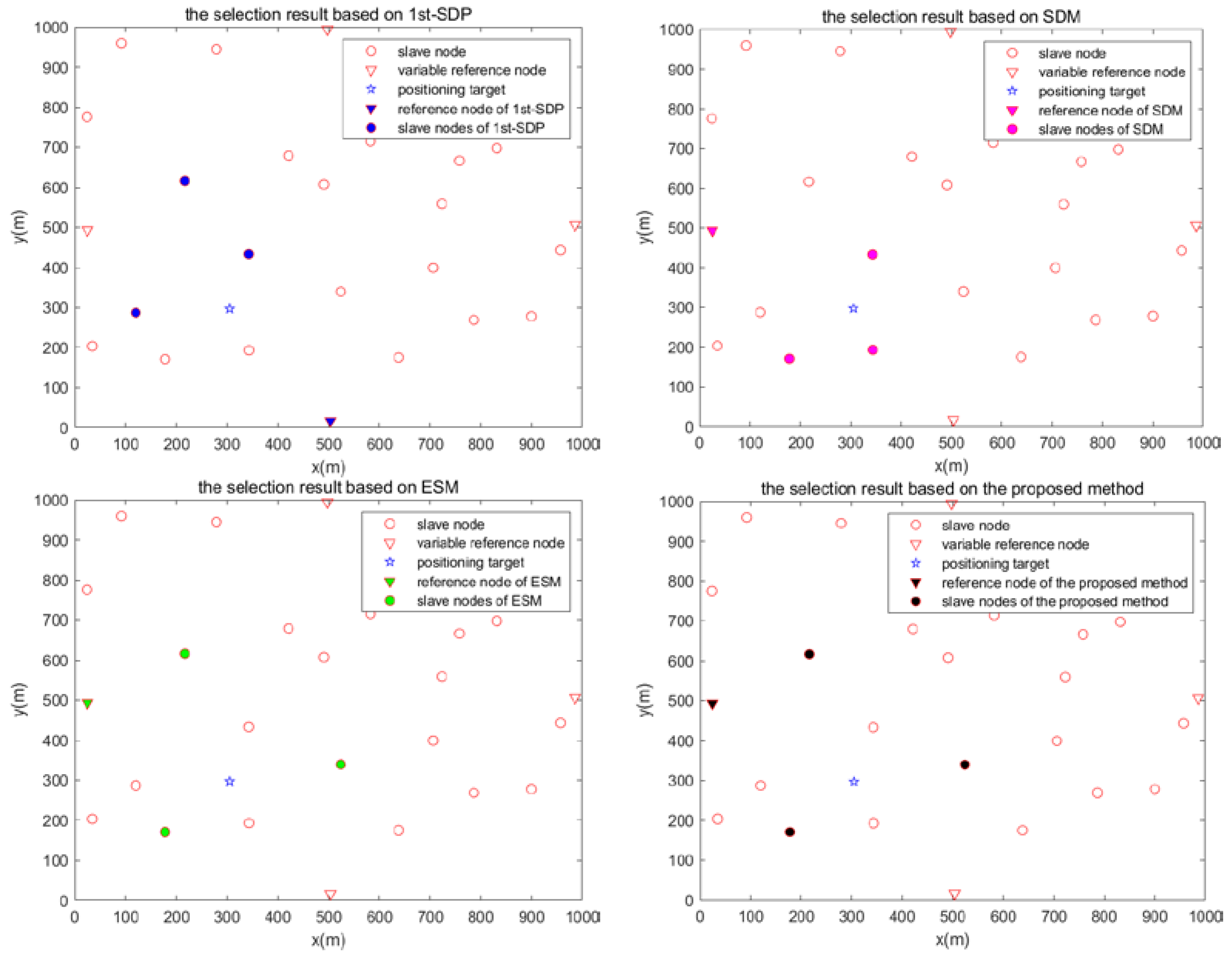
The shortest distance method (SDM) [28], exhaustive search method (ESM) [29], the single determined reference node method (1st-SDP) [30], and the proposed method were used to solve the detection equipment selection problem. The standard deviation of the TDOA measurement error and sensor position error were 3.3 m and 1 mm, respectively. The detection equipment selection results of each method are shown in Figure 8. It is worth noting that the sensor selection results given by the exhaustive search method and the algorithm in this paper were same.

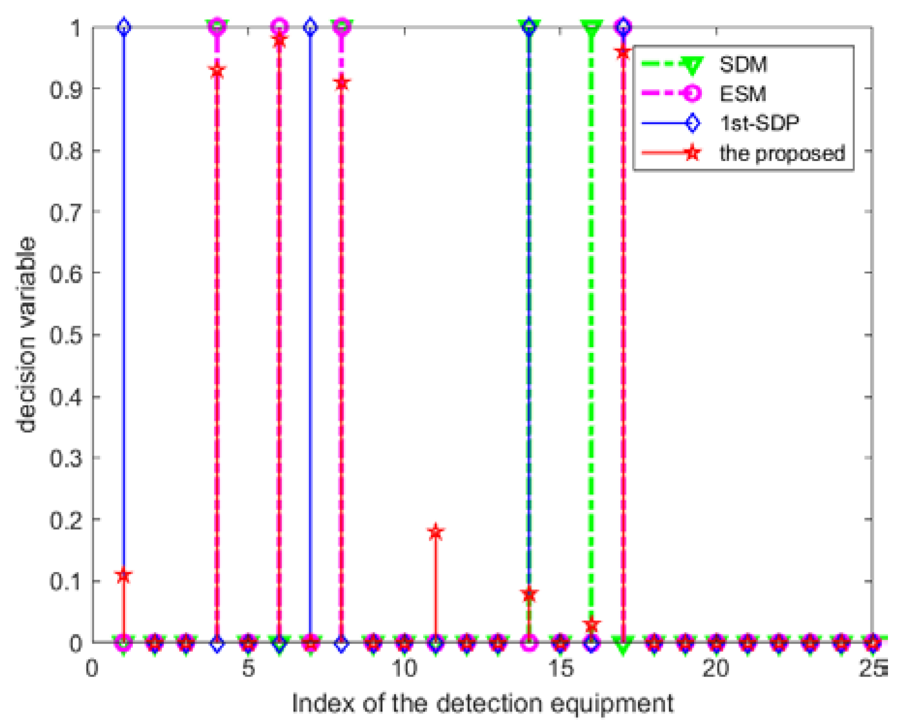
In addition, the serial number of the selected node was given, as shown in Figure 9. The proposed algorithm and exhaustive search method (ESM) chose the same detection equipment. In this work, the proposed algorithm with the shortest distance method (SDM), which had some detection equipment selection, was the same and chose the same reference node. This is because the reference node selection utilized the shortest distance method (derived from AOA coarse position).

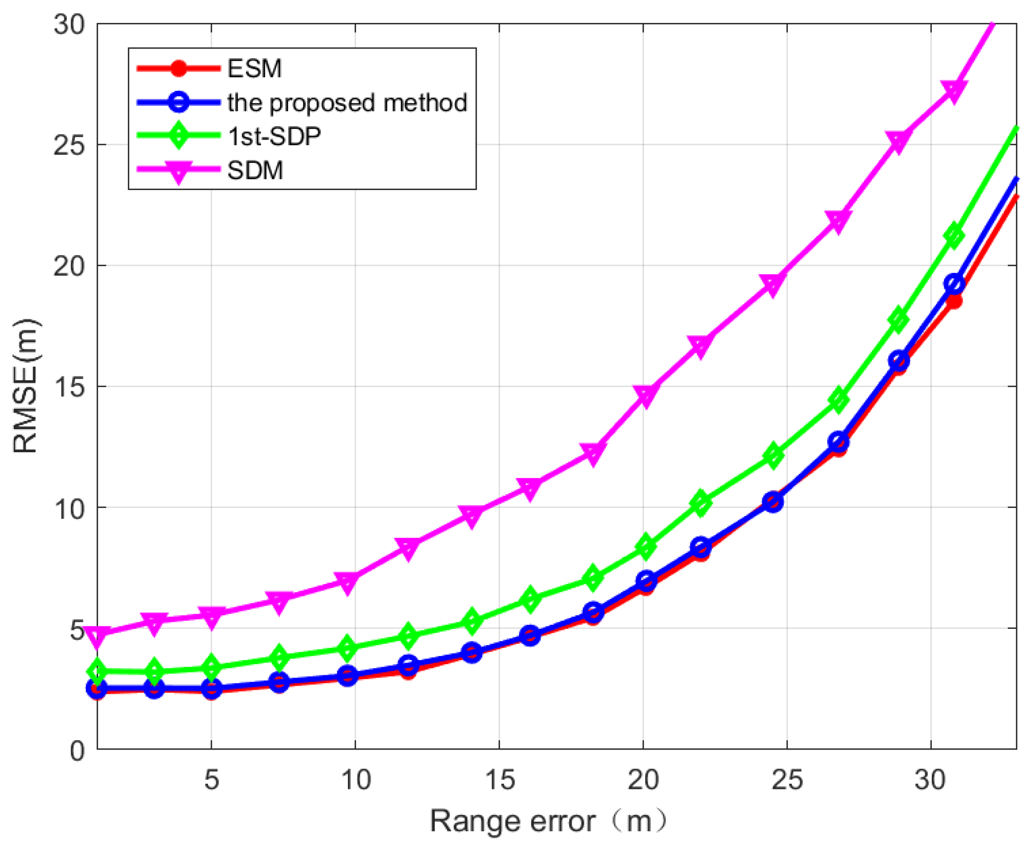
Figure 10 shows the RMSE changes of nodes selected by different selection algorithms when the standard deviation of the R-TDOA measurement error changed from 1 m to 35 m. If not specifically required, a penalty factor was selected as $\lambda =0.01N$. It can be seen from the figure that the detection device selected by the proposed algorithm had better location performance than the results of the shortest distance method (SDM) [28] and the single determined reference node method (1st-SDP) [31] and was closer to the location performance of the exhaustive search method (ESM) [29]. The positioning performance was better than that of 1st-SDP, which also adopted SDP optimization but fixed one main node. Compared with the single reference node SDP optimization algorithm (1st-SDP), the positioning accuracy was improved by 15.8%.

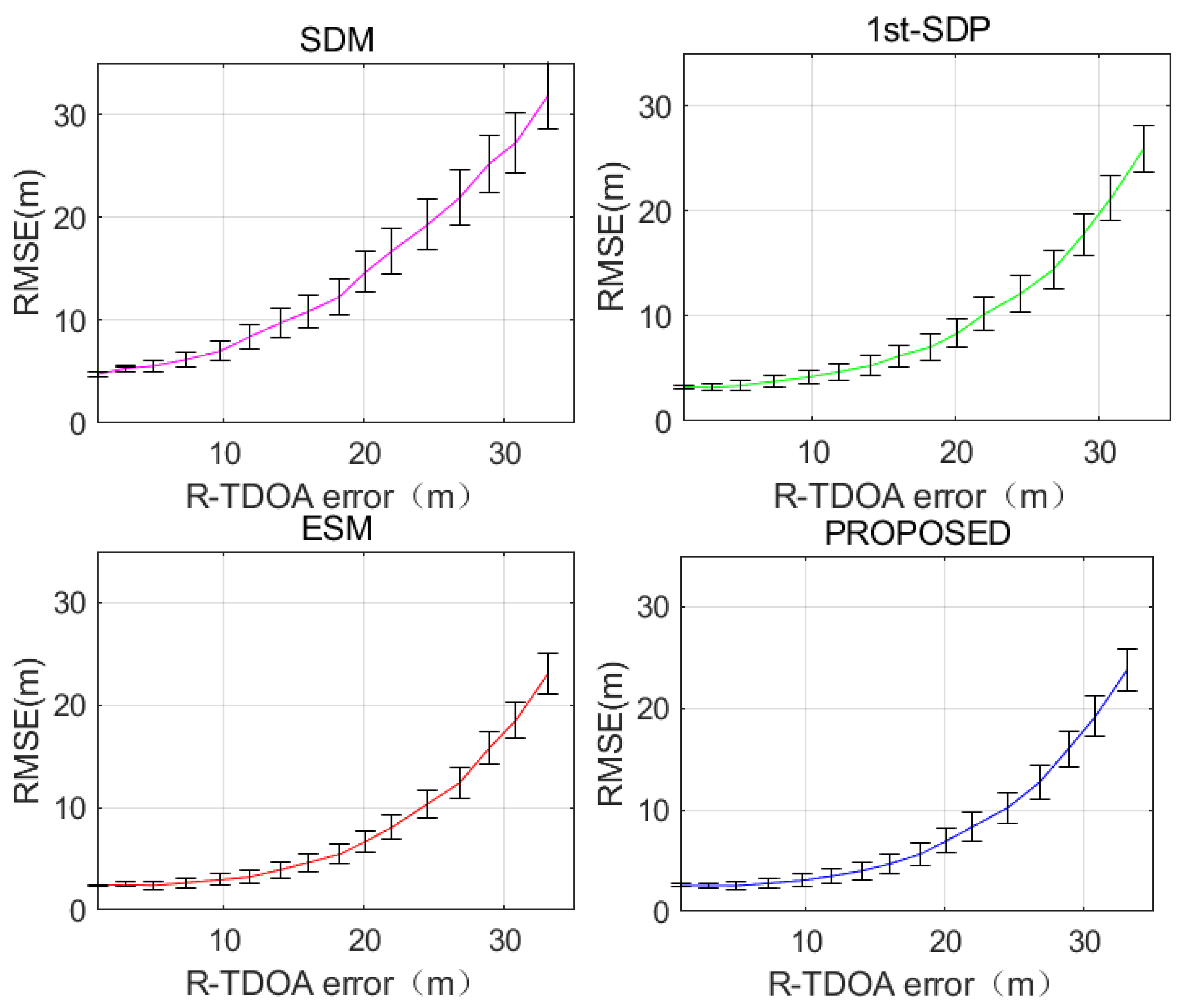
Figure 11 shows the curve of the root mean square error of several algorithms as the TDOA measurement error changes, and the error range is shown in the figure. As can be seen from Figure 10, with the increase in TDOA ranging error, the variation range of root mean square error also increased. Because the same positioning method was adopted, the difference of the error range between the proposed optimization selection method and ESM was not obvious.

Table 1. Running time and root mean square error (N = 25).

Algorithm	Average Running Time(s)	Average RMSE(m)
SDM	38.34	6.99
1st-SDP	36.76	4.21
ESM	289.91	2.96
Proposed	37.56	3.05

shows the average running time required by each method and the root mean square deviation of the running time. When the standard deviation of TDOA measurement error was 10 m and the standard deviation of the detection device position error was 1 m, 200 Monte Carlo experiments were conducted. It can be seen from Table 1 that the detection equipment selected by the exhaustive search method had the smallest positioning error but the largest running time, which was much larger than the other methods. The running time of the other three methods was similar, but the positioning accuracy of the proposed method was the highest, close to the exhaustive search method.

4.4. Analysis of the Accuracy of Optimized Node Selection

After the optimized selection of the detection equipment, there were still errors in solving the location of the target; the error size determined the accuracy of the result. Here, the CRLB value was used to determine whether the location was correct and effective. The method was that the CRLB threshold was given. A value greater than or equal to the threshold was defined as a positioning error, while a value smaller than the threshold was defined as a correct positioning. The positioning selection accuracy of several semi-definite relaxation optimization algorithms is compared below.

The SDR-TDOA method [6], SDR-TOA method [12], 1st-SDP method [31], and SDR-AR-known [14] method were compared with the method proposed in this paper. The total number of nodes in the positioning system varied between $N=20$ and $N=100$. A total of 100 positioning objects were randomly generated and the CRLB of each positioning geometry was calculated. If the CRLB locus of the selected node was greater than 30 m², the selection was considered wrong. 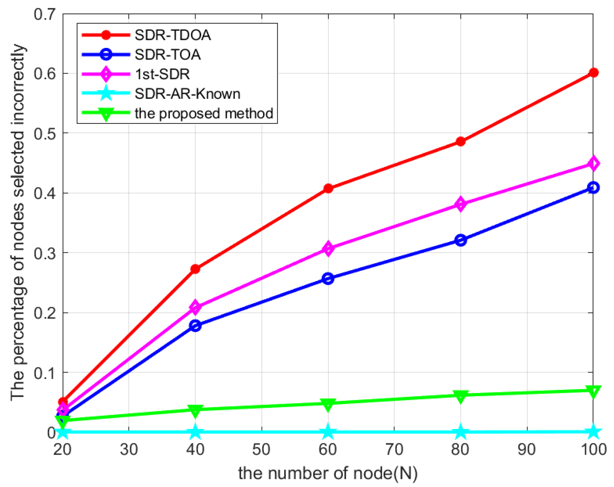Figure 12 shows that as the number of nodes increased, the proportion of incorrect selections increased.

As can be seen from the figure, when the total number of detection devices in the first three methods was N = 100, the proportion of wrong selection exceeded 40%. In comparison, the ratio of the method proposed in this paper to the SDR-AR-known method was less than 10%. The ratio of the method proposed in this paper was slightly higher than that of the SDR-AR-known method because the method proposed in this paper set a specific number of variable detection devices. In the SDR-AR-known method, all nodes can be set as variable nodes, so this result is reasonable. However, for the positioning system in a complex environment with multiple detection devices in a wide area, the method proposed in this paper is a good solution to reduce the cost caused by the number of primary nodes.

5. Conclusions

In this paper, aiming at the problems of limited wireless signal propagation, channel attenuation, and non-line-of-sight propagation in the post-disaster environment, a node selection algorithm combining the main mobile base station and slave detection equipment is proposed to improve the success rate of weak signal acquisition of wide-area target positioning. A positioning system with multiple pieces of detection equipment was constructed and a decision variable with variable nodes was generated. Based on the coarse positioning (AOA) of the target by the variable mobile base station, the penalty function containing distance information was generated to complete the relaxation process of non-convex optimization. Under the condition that the number of optimized nodes was given, the optimal node combination was found by the node selection algorithm based on SDP. By analyzing the influence of a penalty factor on the performance of the optimized node selection algorithm, the penalty factor was selected as $\lambda =0.01N$. Multi-group simulation results showed that its performance was better than that of the shortest distance algorithm and the single reference node SDP optimization algorithm and close to the exhaustive search algorithm. The correct selection rate of locating nodes was higher than 90%. Compared with the single reference node SDP optimization algorithm, the positioning accuracy was improved by 15.8%. The running time of each algorithm increased with the increase in the number of nodes, especially the exhaustive search method. When the number of nodes in the system was N = 25, the detection equipment selected by the exhaustive search method had the smallest positioning error with the largest running time. The running time of the other three methods was similar, but the positioning accuracy of the proposed method was the highest, close to the exhaustive search method.