Trigger-Based K-Band Microwave Ranging System Thermal Control with Model-Free Learning Process

Abstract

Micron-level accuracy K-band microwave ranging in space relies on the stability of the payload thermal control on-board; however, large quantities of thermal sensors and heating devices around the deployed instruments consume the precious inner communication resources of the central computer. Another problem arises, which is that the payload thermal protection environment can deteriorate gradually through years operating. In this paper, a new trigger-based thermal system controller design is proposed, with consideration of spaceborne communication burden reduction and actuator saturation, which guarantees stable temperature fluctuations of microwave payloads in space missions. The controller combines a nominal constant sampling PID inner loop and a trigger-based outer loop structure under constraints of heating device saturation. Moreover, an iterative model-free reinforcement learning process is adopted that can approximate the estimation of thermal dynamic modeling uncertainty online. Via extensive experiment in a laboratory environment, the performance of the proposed trigger thermal control is verified, with smaller temperature fluctuations compared to the nominal control, and obvious efficiency in system communications. The online learning algorithm is also tested with deliberate thermal conditions that deviate from the original system—the results can quickly converge to normal when the thermal disturbance is removed. Finally, the ranging accuracy is tested for the whole system, and a 25% (RMS) performance improvement can be realized by using a trigger-based control strategy—about 2.2 µm, compared to the nominal control method.

1. Introduction

K-band microwave ranging (MWR) technology can provide micron-level precise ranging measurements between spacecraft in space, which has potential applications in the fields of Earth elevation surveying, gravity field detection, and other space missions [1,2]. The accuracy ranging performance (time delay) of the MWR system is mainly affected by the payload thermal condition in space. The state-of-the-art payload thermal controller should be well designed with tiny temperature fluctuations during orbiting; however, the spacecraft thermal control system is a large-scale system that involves hundreds, even thousands of temperature sensors and patch heaters around instruments, which increases the pressure on communication with the on-board central computer when engaged in diversified space missions in the future [3,4,5]. At the same time, the thermal control system itself can be deteriorated to the original dynamic model during multiple year-long space missions, and the adaptive approaches should be adopted to dealing with this situation. To deal with such problems, in this paper, a new thermal control strategy is proposed that is based on triggered sampling and the model-free learning process.

The event-triggered control (ETC), in contrast to the traditional time trigger control with fixed sampling period, adopts the updating strategy of sampling in a variable period [6,7,8]. Designers can impose certain thresholds with performance indexes for the system according to actual needs. The control signals are transmitted and updated inside the system only when the states exceed the threshold conditions [9,10]. Zhang [11] embedded ETC into a linear system model to address predictive control problems, updating the predictive sampling step-time through a fixed-threshold event-triggering mechanism. In [12], the design of the multi-variable linear industrial process ETC with time delay and quantization error is studied, the controller parameters are calculated by linear matrix inequality (LMI), and the closed-loop system asymptotic stability proof using Lyapunov theory is provided. Azimi [13] proposed an ETC design that considered the system transmission delay and packet loss during the signal transmission in the chemical process, which can track the set values of the system with the signal transmission constrain. For the situation of time-varying model parameters of linear chemical control process in different working environments, Li [14] described the uncertain system by using Markov random theory, and an event-triggered sliding mode controller with finite-time convergence is designed by combining homogeneous theory with an event-triggered mechanism, which realized the finite-time convergence. The thermal control system we considered in this paper includes a saturated actuator process, which is a type of nonlinear system—scholars have also focused on the application of ETC to nonlinear systems. References [15,16] analyzed the nonlinear strict feedback system and uncertain strict feedback nonlinear system according to adaptive control theory. The results show that a control system with an event-triggering mechanism can improve the transmission efficiency of the signal—it can also reduce the energy consumption and cost. Abhinav [17] designed an adaptive event triggered sliding mode controller by combining the sliding mode control with ETC, and the results show that the designed controller has good regulating performance in the presence of external disturbances and model uncertain. Moreover, the unknown nonlinear characteristics inside the dynamics model can also be approximated by advanced control methods, such as fuzzy control [18], neural network [19,20,21], and adaptive dynamic programming (ADP) [22]. References [23,24] considered the ADP triggering problem with a saturated actuator. Seuret [25] adopted the linear quadratic optimal control method. Reference [26] provided a stability analysis of the system with disturbance. Reference [27] introduced inequality to analyze the trigger system.

A thermal system using an ETC design relies on the temperature sensors as state-sampling hardware, which can diverge from the tracking trajectory once measurement malfunctions. Some scholars have proposed the idea of self-triggered control (STC) in recent years [28,29,30,31,32]. The principle of STC is to actively predict when the next triggering time will occur according to the previously received data and system dynamics. Compared with ETC, STC reduces the transmission times of the feedback signals, effectively reduces the on-board data transmission burden, and improves the control efficiency. Wang [33] provided the self-triggering conditions of general linear systems based on the Lyapunov method. Almeida [34] studied the self-triggering of linear systems with bounded disturbance state feedback to ensure the system asymptotic stability. The application of STC to a network control system is proposed in [35].

The triggered control strategy design may improve the on-board communication efficiency most of time, relying on the system model functioning well; however, as the observation platform for long-term space missions is critical, the spacecraft payload thermodynamic will gradually deteriorate over time, which will clearly deviate from the originally designed model. As a typical intelligent agent in space with sensing and action functions, the spacecraft platform malfunction should be detected and calibrate itself on-orbit, and methods such as optimal control and dynamic programming should be adopted for this model’s uncertain situation.

Recently, efficient approximation techniques have been proposed to solve the above described problem, known as approximate dynamic programming (ApDP) or reinforcement learning (RL), including value-based RL (Q-learning methods) [36,37], policy-based RL (policy gradient methods) [38,39,40], and value-policy combined RL (actor-critic methods) [41]. For systems with disturbed dynamics, LQR has been widely used for learning-based controller design [42,43,44]. Lee [45] has developed a Q-learning framework for LQR control based on an alternative optimization formulation of the problem. The proposed framework is then used to design a model-free Q-learning algorithm based on primal dual updates. Policy gradient methods continuously calculate the gradient of the cumulative income of the agent and the strategy parameters under the current strategy in an end-to-end approach, and finally the gradient converges to the optimal strategy [38]. The actor-critic methods include two parts: actor and critic, in which the actor is responsible for interacting with the environment and selecting actions based on strategy function; the critic is based on the value function, which is responsible for evaluating the actor and guiding its next action. In the actor-critic algorithm, it is necessary to approximate the strategy function and the value function independently [46]. Basically, the critic calculates the state optimal value, and the actor uses it to iteratively update the parameters of the strategy function, selecting action, so as to obtain the immediate reward and move to the next state. The critic uses the reward and the new state to update the parameters of the value function.

The application of RL to spacecraft thermodynamic systems is rarely reported in recent years, according to the authors’ literature review. Lee [47] introduced a RL-based model-free predictive control structure for chiller plants. Qiu [48] provided an optimal operation solution of chillers by combining RL technique and expertise knowledge, aiming for a balance of power and indoor comfort. Inspired by the literature, this paper focuses on a trigger-based MWR payload thermal control system design with an online learning iteration, aiming to the micron-level precise ranging performance in space missions [49,50]. The proposed approach benefits from the following noteworthy features:

• Feasible triggered thermal system control design with obvious communication burden reduction;
• No original thermodynamic information required when faced with disturbed system model uncertainty;
• Suitable for real autonomous management of space platforms with long-term mission life;
• Thermal control strategies can be selected from nominal control, triggered control, and model-free learning process, according different orbiting period.

The rest of the paper is organized as follows: Section 2 provides the thermal system modeling for the micron-level K-band ranging system with efficient saturation trigger feedback controller design. The model-free learning method is shown in Section 3 for the case of thermal system uncertainty. Finally, the experimental results in a laboratory environment are provided, which demonstrate the effectiveness of the proposed method.

2. Thermal System Design for Precise Ranging System

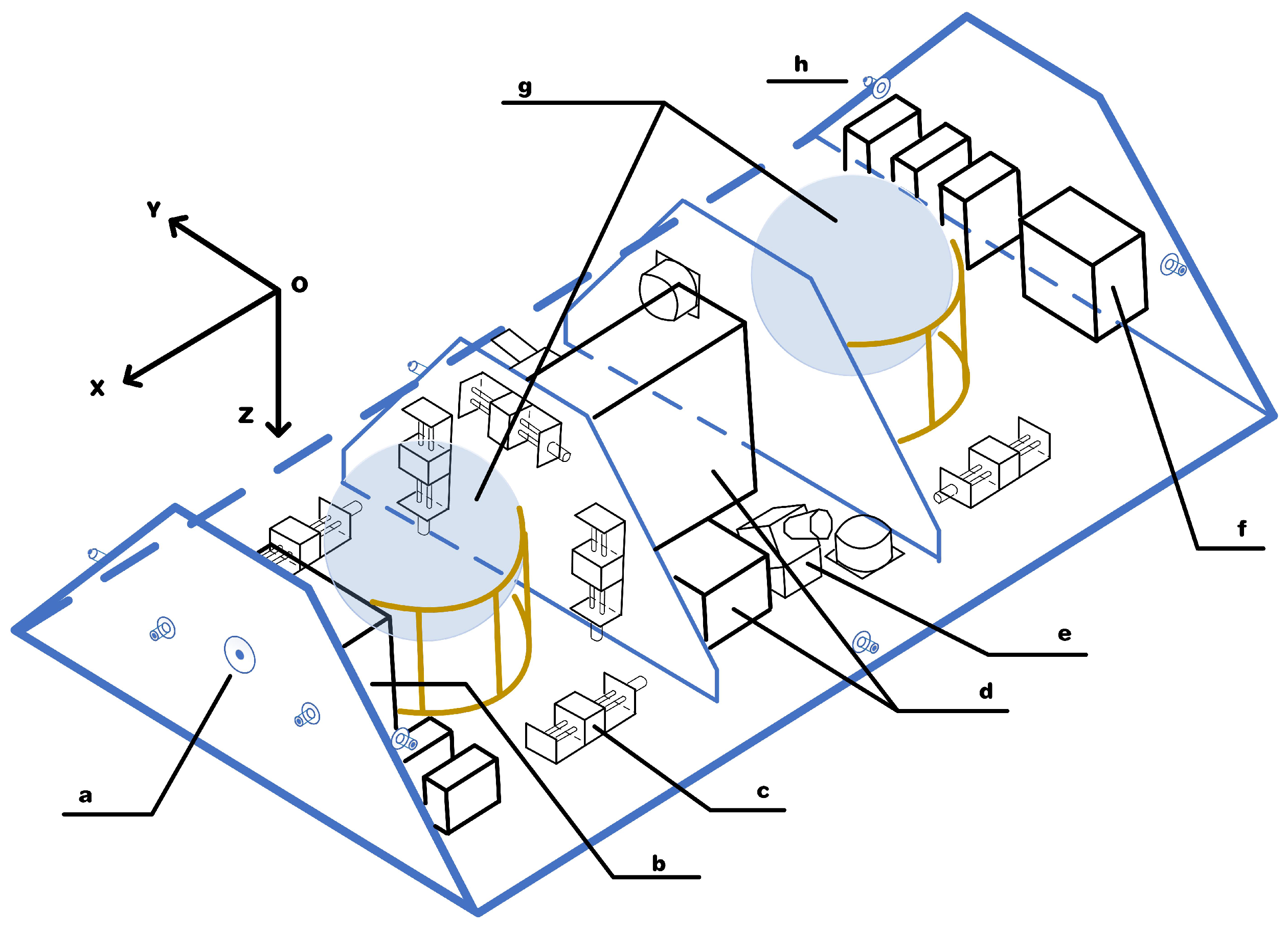
2.1. Thermal Structure of Deployed Satellite

The main sources of heat during a satellite orbiting in space including sunlight, thruster ignition, and power consumption of on-board electric devices. The fluctuation of satellite temperature has the following characteristics: temperature, both daily and seasonal, periodically changes as the Earth rotates and revolves around the sun; On the other hand, on-board electric devices will also cause temperature changes due to work status changes, failures, or other uncertain factors, as the on-board thermally insulated layer performance decreases with satellite aging. In order to obtain a proper heat transfer and conversion, avoiding the temperature exceeding the normal working range, thermal control technology should be adopted that includes specially designed active and passive approaches.

The structure of the whole satellite is shown in Figure 1 below, in which “b” indicates the installed position of the MWR system, which includes four parts: K-band transceiving antenna, waveguide switch network, signal process unit, and ultra-stable crystal oscillator (USO), which constitutes the micron-level microwave ranging system as a whole.

It can be seen from Figure 1 that the whole ranging system is installed on the +X and +Z panels of the satellite. A three-level thermal protection structure is designed in order to prevent the payload from being affected by space radiation during operation. First, the platform outer shield, with bare carbon fiber reinforced plastic (CFRP) with 10-layer multi-layer insulation (MLI) pack, is used that can block any heat from leaking in from the outer solar panel. Second, the payload cabin, with CFRP with single layer Kapton foil, is used, which can minimize radiative heat from the inner platform environment to the MWR payload enclosure. Moreover, there is thermal insulation between the satellite platform and the payload, which is made of low conductive material to reduce the effect of temperature variations at the structure interface. The internal thermal conduction balance treatment is carried out within deployed cabins for the differential temperature caused by on-orbit illumination directions on the surface of the satellite. Third, active thermal control, with dedicated heaters and condensation heat pipes, is used for critical payloads that have more stringent temperature limits than the rest of the spacecraft—mainly the four parts of the MWR system. The temperatures of the MWR equipment are monitored using sensors and maintained within the desired limits by several patch heaters and phase-changed heat pipes that are controlled by the spacecraft central computer during the stages of science operations.

According to the massive data from previous tests, the ranging error of the MWR equipment is mainly due to the microwave measurement signal chain, which includes: (1) the temperature fluctuation of USO that reduces the clock frequency stability; (2) the thermal deformation of the horn antenna may lead to changes in the antenna phase center; (3) temperature changes of phase-locked frequency doubling equipment, microwave network, quadrature mixer, intermediate frequency amplifier, and low-pass filter may induce errors in the ranging measurement result. As a result, it is necessary to improve the accuracy and stability of temperature control for these devices, which could be improved using less than ±0.15 K/orbit. In addition, the digital signal processing unit of MWR also needs high-precision temperature control within ±0.1 K/orbit, since it contains the A/D converter of the low-pass filtered signal, FPGA, and DSP components on the same circuit board, which are highly sensitive to temperature fluctuations.

2.2. Payload Thermal Dynamic Modeling and Nominal PID Control

The temperature of deployed payloads is directly related to its surrounding environment of satellite platform in space and internal thermal exchange between themselves. With a proper structure design featuring three levels of thermal protection, the payloads can be perform well within finite temperature fluctuations inside a cabin room. In this paper, we consider the thermal coupling relationship between those payload components; the thermal analysis adopts the node network method to establish the thermal balance equation of any node on satellite as follows [51]:

$$c_i{m}_i\frac{d{T}_i}{dt}+{ϵ}_i{a}_i\left(T_i-T_{Ti}\right)=q_i$$

(1)

where the subscript i denotes the thermal nodes, $c_i$ denotes the specific heat capacity of the payload metal alloy block, $m_i$ denotes the block mass, $T_i$ denotes the transient thermal temperature, $T_{Ti}$ is target temperature, ${ϵ}_i$ denotes the average heat transfer coefficient of each node, $a_i$ is the area of each heat patch/pipe surface, and $q_i$ is the heating/cooling power of each node around payload. The thermal control is realized by several heating and condensation patch nodes with an adiabatic section around each payload components, providing the heating and cooling actions from control command. Typical electric heating is used when the temperature is below the target, and the state-of-the-art micro-electro-mechanical system (MEMS)-based pulse width modulation (PWM) high-speed on-off valve is used to cool the liquid flow inside the phase change pipe during high temperature stages.

For the purpose of fast and stable internal temperature control of payloads during space missions, especially during precise ranging stages, two cycles of a closed-loop active thermal controller are designed: one is a high-power electric heating/cooling controller with temperature sensors patched around payloads using PID control; the other one is a precise low-power heating controller using optimal control with triggering saturation constraints.

A typical PID control algorithm is used as a nominal scheme given as [52,53,54]:

$$\mathbf{u}\left(t\right)=K_p\left[\mathbf{e}\left(t\right)+\frac{1}{K_I}\sum _{\tau =0}^t\mathbf{e}\left(\tau \right)·T_s+K_D\frac{\mathbf{e}\left(t\right)-\mathbf{e}\left(t-1\right)}{T_s}\right]$$

(2)

where $K_p,K_I,K_D$ are the coefficients of proportional, integral, and differential, respectively; $T_s$ is sampling time, $\mathbf{e}\left(t\right)$ is the difference of measured temperature and target temperature, and $\mathbf{u}\left(t\right)$ is the heating/cooling power consumption for active thermal control.

2.3. Trigger-Based Precise Optimal Thermal Control with Saturation Constraint

The thermal dynamic model and PID algorithm design above aim to provide the nominal thermal active control during the space orbiting period. For the purpose of the high-precision microwave ranging system that is functional during the science observing phase in space, each payload component is patched around several heating/cooling nodes and measurement sensors in order to fully realize thermal control and temperature monitoring.

Here, we want the thermal control system to be tracking the desired temperatures during the space mission with minimal control burdens. First, considering the nominal states as $\mathbf{x}={\left[\begin{array}{cccc}{T}_a& T_w& T_m& T_u\end{array}\right]}^T$, where the subscript $a,w,m,u$ mean the four MWR components of the K-band antenna, waveguide switch network, microwave signal process unit, and USO. Define the new states as the difference of current states $\mathbf{x}\left(t\right)$ and $\mathbf{x}\left(t_f\right)$, namely, $\mathit{x}\left(t\right)\stackrel{\Delta }{=}\mathbf{x}\left(t\right)-\mathbf{x}\left(t_f\right)$ with $\mathit{x}={\left[\begin{array}{cccc}\delta T_a& \delta T_w& \delta T_m& \delta T_u\end{array}\right]}^T$. Similarly, we can define the heating/cooling control variable $\mathit{u}\left(t\right)\stackrel{\Delta }{=}\mathbf{u}\left(t\right)-\mathbf{u}\left(t_f\right)$ with $\mathit{u}={\left[\begin{array}{cccc}\delta q_a& \delta q_w& \delta q_m& \delta q_u\end{array}\right]}^T$ according to the deviation between the actual and the nominal thermal control input. On the premise of a given nominal temperature state sequence, the time series of the nominal control input can be obtained directly through the PID algorithm; so, after the control input $\mathbf{u}={\left[\begin{array}{cccc}{q}_a& q_w& q_m& q_u\end{array}\right]}^T$ of the deviation dynamics is solved, the actual temperature tracking control can be obtained through the summation of $\mathbf{u}$ and $\mathit{u}$.

The precise thermal control is realized through several accuracy calibrated patch heater and cooler, with limited power consumption constraints. Here, we consider the deviation thermal system as a saturated linear dynamic equation of the form:

$$\begin{array}{c}\dot{\mathit{x}}\left(t\right)=\mathit{A}\mathit{x}\left(t\right)+\mathit{B}\sigma \left(\mathit{u}\left(t\right)\right),\mathit{x}\left(t_0\right)={\mathit{x}}_0,t\ge 0\hfill \\ \mathit{u}\left(t\right)=\mathit{K}\mathit{x}\left(t_k\right),t\in \left[t_k,t_{k+1}\right)\hfill \end{array}$$

(3)

where $\mathit{A}\in {\mathbb{R}}^{n\times n}$ is the state matrix, and $\mathit{B}\in {\mathbb{R}}^{n\times m}$ is the control matrix. $\mathit{K}=-{\mathit{R}}^{-1}{\mathit{B}}^T\mathit{P}\in {\mathbb{R}}^{m\times n}$ denotes the feedback gain matrix through optimal control. Here, we assume that all states are observable and that the system is controllable. Because of the unmodeled dynamics and external thermal disturbances during on-orbit mission flight, $\mathit{A}$ and $\mathit{B}$ are both disturbed matrices.

Note here we define the saturation control of $\sigma \left({\mathit{u}}_i\right)\stackrel{\Delta }{=}sign\left({\mathit{u}}_i\right)·min\left\{{\overline{\mathit{u}}}_i,\left|{\mathit{u}}_i\right|\right\}$, where ${\mathit{u}}_i$ is the i-th control input signal and ${\overline{\mathit{u}}}_i$ is the maximum amplitude of i-th control actuator, i.e., the heating/cooling power. The time-tag $t_k$ shows up through the event trigger, meaning the control signal triggers off at time $t_k$, and holds still during time period $t\in \left[t_k,t_{k+1}\right)$; this can greatly save signal transmitting bandwidth, reducing the communication burden for the whole on-board system.

Next, we give a brief introduction of the optimal control used in this paper. The tracking performance of the energy cost is written as:

$$J\left(\mathit{x},\mathit{u},t_0,t_f\right)=\frac{1}{2}{\mathit{x}}^T\left(t_f\right)\mathit{P}\left(t_f\right)\mathit{x}\left(t_f\right)+\frac{1}{2}{\int }_{t_0}^{t_f}\left({\mathit{x}}^T\left(\tau \right)\mathit{M}\mathit{x}\left(\tau \right)+{\mathit{u}}^T\left(\tau \right)\mathit{R}\mathit{u}\left(\tau \right)\right)d\tau$$

(4)

where $\mathit{P}\left(t_f\right)\in {\mathbb{R}}^{n\times n}$ is the solution of the Riccati equation in time $t_f$, $\mathit{M}\in {\mathbb{R}}^{n\times n}\succ =0$, $\mathit{R}\in {\mathbb{R}}^{m\times m}\succ 0$. Suppose we have the matrix pairs $\left(\mathit{A},\mathit{B}\right)$ controllable and $\left(\sqrt{\mathit{M}},\mathit{A}\right)$ measurable, clearly, we will obtain the best performance with minimal value of J, and the final object of control system is finding the optimal value $V^{*}$ with dynamic modeling disturbances:

$$V^{*}\left(\mathit{x},t_0,t_f\right)=\underset{\mathit{u}}{min}\left[J\left(\mathit{x},\mathit{u},t_0,t_f\right)\right]$$

(5)

The finite horizon optimal control problem can be solved as follows: define the Hamiltonian function

$$H=\frac{1}{2}\left({\mathit{x}}^T\left(t\right)\mathit{M}\mathit{x}\left(t\right)+{\mathit{u}}^T\left(t\right)\mathit{R}\mathit{u}\left(t\right)\right)+\frac{\partial V^{*T}}{\partial \mathit{x}}\left(\mathit{A}\mathit{x}\left(t\right)+\mathit{B}\mathit{u}\left(t\right)\right)$$

(6)

With proper derivation, the following HJB equation can be obtained [55]:

$$-\frac{\partial V^{*}}{\partial t}=\frac{1}{2}\left({\mathit{x}}^T\left(t\right)\mathit{M}\mathit{x}\left(t\right)+{\mathit{u}}^{*T}\left(t\right)\mathit{R}{\mathit{u}}^{*}\left(t\right)\right)+\frac{\partial V^{*T}}{\partial \mathit{x}}\left(\mathit{A}\mathit{x}\left(t\right)+\mathit{B}{\mathit{u}}^{*}\left(t\right)\right)$$

(7)

Then, we have the optimal control of

$${\mathit{u}}^{*}\left(\mathit{x},t\right)=-{\mathit{R}}^{-1}{\mathit{B}}^T\mathit{P}\left(t\right)\mathit{x}\left(t\right)=\mathit{K}\mathit{x}\left(t\right)$$

(8)

where $\mathit{P}\left(t\right)$ can be found in the Riccati equation of

$$\mathit{M}+\mathit{P}\left(t\right)\mathit{A}+{\mathit{A}}^{T}P\left(t\right)-\mathit{P}\left(t\right)\mathit{B}{\mathit{R}}^{-1}{\mathit{B}}^T\mathit{P}\left(t\right)=0$$

(9)

Theorem 1.

Suppose we have $\mathit{P}\left(t\right)$ from Equation (9), with the condition of $\mathit{P}\left(t_f\right)$, then we can obtain the optimal control of Equation (8), satisfying the minimal function of Equation (5). Moreover, the origin point is the globally uniformly asymptotically stable equilibrium point for the closed-loop system.

Proof of Theorem 1.

The proof can be found in ref [55], which is not shown here. □

2.4. Trigger Condition Analysis

We define $\mathit{e}\left(t\right)=\mathit{x}\left(t_k\right)-\mathit{x}\left(t\right)$, meaning the state differences of the previous triggered time and current time. The sampling signal of the system that is sent to the controller through feedback needs to meet the selected trigger condition. Here, we design the trigger mechanism as:

$$t_{k+1}=t_k+min\left\{{\tau }_k|Z_1\wedge Z_1,\tau >0\right\}$$

(10)

where $Z_1={\mathit{e}}^T\left(t_k+\tau \right)\mathit{S}\mathit{e}\left(t_k+\tau \right)\ge \gamma {\mathit{x}}^T\left(t_k\right)\mathit{D}\mathit{x}\left(t_k\right)+\delta$, $Z_2={∥\sigma \left(\mathit{u}\left(t\right)\right)∥}^2<{\overline{\mathit{u}}}^2$, and $\gamma ,\delta$ are given positive constants, $\mathit{S},\mathit{D}$ are a positive defined matrix, $t_k$ denotes the triggered time of event k, and ${\tau }_k$ the signal transmitting period since $t_k$. Equation (10) can be explained as follows: suppose the first trigger happened in time $t_0$ in a real system operation, and after that, no trigger happened even if condition $Z_1$ is satisfied, with the control signal under saturation, i.e., condition $Z_2$. By achieving this, it will greatly improve the communication resource utilization of the system.

Let $\delta =0$, and $\mathit{S}=\mathit{D}=\mathit{P}$; we have the event-trigger condition of

$$\left\{{\mathit{e}}^T\left(t\right)\mathit{P}\mathit{e}\left(t\right)\ge \gamma {\mathit{x}}^T\left(t_k\right)\mathit{P}\mathit{x}\left(t_k\right)\right\}\wedge \left\{{∥\sigma \left(\mathit{u}\left(t\right)\right)∥}^2<{\overline{\mathit{u}}}^2\right\},t>t_k$$

(11)

The event-trigger transmission condition is realized by hardware samplings and trigger condition judgment. Similarly, the self-trigger is implemented through previous signal and state predictions. Here, we explain the self-trigger conditions as follows: consider time $t\in \left[t_k,t_{k+1}\right)$, by using the system model of Equation (3), we have

$$\begin{array}{c}\dot{\mathit{e}}\left(t\right)=-\dot{\mathit{x}}\left(t\right)=\mathit{A}\mathit{e}\left(t\right)-\left[\mathit{A}\mathit{x}\left(t_k\right)+\mathit{B}\sigma \left(\mathit{K}\mathit{x}\left(t_k\right)\right)\right]\stackrel{\Delta }{=}\mathit{A}\mathit{e}\left(t\right)-\mathit{X}\hfill \\ \mathit{x}\left(t_k\right)=0,t>t_k\hfill \end{array}$$

(12)

The analytical solution of Equation (12) is given as

$$\begin{array}{c}\hfill \mathit{e}\left(t\right)=-{\int }_{t_k}^t{\mathit{e}}^{\mathit{A}(t-\tau )}d\tau ·\mathit{X}=-{\int }_0^{t-t_k}{\mathit{e}}^{\mathit{A}s}ds·\mathit{X}\end{array}$$

(13)

With proper derivation, we have

$$\begin{array}{ccc}\hfill {\mathit{e}}^T\left(t\right)\mathit{P}\mathit{e}\left(t\right)& =& {\left\{{\int }_0^{t-t_k}{\mathit{e}}^{\mathit{A}s}ds·\mathit{X}\right\}}^T\mathit{P}\left\{{\int }_0^{t-t_k}{\mathit{e}}^{\mathit{A}s}ds·\mathit{X}\right\}\hfill \\ & \le & {\left\{{\int }_0^{t-t_k}{\mathit{e}}^{{\lambda }_{max}\left(\mathit{A}\right)s}ds\right\}}^2·{\mathit{X}}^T\mathit{P}\mathit{X}\hfill \end{array}$$

(14)

Let $\xi \left(\mathit{x}\left(t_k\right)\right)={\mathit{X}}^T\mathit{P}\mathit{X}$, and $\theta \left(\mathit{x}\left(t_k\right)\right)={\lambda }_{min}\left(\mathit{P}\right){∥\mathit{x}\left(t_k\right)∥}^2$. According to Equation (11), we can obtain the self-trigger time-tag of $t_{k+1}$ through

$$\left\{{\left[{\int }_0^{t_{k+1}-t_k}{\mathit{e}}^{{\lambda }_{max}\left(\mathit{A}\right)s}ds\right]}^2\xi \left(\mathit{x}\left(t_k\right)\right)=\gamma \theta \left(\mathit{x}\left(t_k\right)\right)\right\}\wedge \left\{{∥\sigma \left(\mathit{u}\left(t\right)\right)∥}^2<{\overline{\mathit{u}}}^2\right\}$$

(15)

Clearly, Equation (15) is obtained based on the event-trigger condition of Equation (11), with less trigger period. Finally, we can obtain the self-trigger condition of

$$t_{k+1}=t_k+h\left(\gamma ,\mathit{x}\left(t_k\right)\right)$$

(16)

The self-trigger time-tag of $t_{k+1}$ meaning the sampling point, according to saturation function, and the feedback of system states in $t_{k+1}$ depending on ${∥\sigma \left(\mathit{u}\left(t\right)\right)∥}^2<{\overline{\mathit{u}}}^2$. Moreover, the trigger period of $h\left(\gamma ,\mathit{x}\left(t_k\right)\right)$ relies on matrix $\mathit{A}$, namely:

(1) if ${\lambda }_{max}\left(\mathit{A}\right)=0$, then we have ${\int }_0^{t_{k+1}-t_k}{\mathit{e}}^{{\lambda }_{max}\left(\mathit{A}\right)s}ds={\int }_0^{t_{k+1}-t_k}ds$, and

$$h\left(\gamma ,\mathit{x}\left(t_k\right)\right)={\left[\frac{\gamma \theta \left(\mathit{x}\left(t_k\right)\right)}{\xi \left(\mathit{x}\left(t_k\right)\right)}\right]}^{1/2}$$

(17)

(2) if ${\lambda }_{max}\left(\mathit{A}\right)\ne 0$, then we have

$$\begin{array}{ccc}\hfill {\int }_0^{t_{k+1}-t_k}{\mathit{e}}^{{\lambda }_{max}\left(\mathit{A}\right)s}ds& =& \frac{1}{{\lambda }_{max}\left(\mathit{A}\right)}{\int }_0^{t_{k+1}-t_k}{\mathit{e}}^{{\lambda }_{max}\left(\mathit{A}\right)s}d{\lambda }_{max}\left(\mathit{A}\right)s\hfill \\ & =& \frac{1}{{\lambda }_{max}\left(\mathit{A}\right)}\left[{\mathit{e}}^{{\lambda }_{max}\left(\mathit{A}\right)(t_{k+1}-t_k)}-1\right]\hfill \end{array}$$

(18)

and

$$h\left(\gamma ,\mathit{x}\left(t_k\right)\right)=\frac{1}{{\lambda }_{max}\left(\mathit{A}\right)}ln\left\{1+{\lambda }_{max}\left(\mathit{A}\right){\left[\frac{\gamma \theta \left(\mathit{x}\left(t_k\right)\right)}{\xi \left(\mathit{x}\left(t_k\right)\right)}\right]}^{1/2}\right\}$$

(19)

Finally, here we provide the schematic diagram of the proposed trigger-based thermal control system as in Figure 2.

2.5. Stability Analysis of Trigger Control

For the given known stable open-loop system, the global stability of the whole system can be guaranteed by selecting appropriate event triggering conditions when the actuator of the system is saturated. Here, we analyze the trigger conditions that can guarantee the global input-state stability of the system. First, considering the system model as in Equation (3), we introduce Lemma 1 and Lemma 2 as:

Lemma 1

([26]). (Input-states stable) for a system as

$$\dot{\mathit{x}}\left(t\right)=f\left(t,\mathit{x},\mathit{u}\right)$$

(20)

where f:$\left[0,\infty \right)\times {\mathbb{R}}^n\times {\mathbb{R}}^m$ is continuous function of t, regional Lipschitz function of $\mathit{x},\mathit{u}$. Let the continuous differentiable function be $V:\left[0,\infty \right)\times {\mathbb{R}}^n\to \mathbb{R}$, which satisfies

$$\underline{\alpha }\left(∥\mathit{x}∥\right)\le V\left(t,\mathit{x}\right)\le \overline{\alpha }\left(∥\mathit{x}∥\right)$$

(21)

$$\frac{\partial V}{\partial \mathit{x}}f\left(t,\mathit{x}\right)\le -\alpha \left(∥\mathit{x}∥\right)+\beta \left(∥\mathit{u}∥\right)$$

(22)

where $\underline{\alpha },\overline{\alpha },\alpha ,\beta$ are $K_{\infty }$ function, then system (20) is input-state stable.

Lemma 2

([26]). For any $\mathit{v},\mathit{w}\in {\mathbb{R}}^m$, if $\mathit{v},\mathit{w}$ belong to linear region $L\left(\mathit{v}-\mathit{w},\overline{\mathit{u}}\right)$, then we have

$${\varphi }^T\left(\mathit{v}\right)\mathit{T}\left(\varphi \left(\mathit{v}\right)+\mathit{w}\right)\le 0$$

(23)

for any positive defined matrix $\mathit{T}\in {\mathbb{R}}^{m\times m}$, where $\varphi \left(\mathit{v}\left(t\right)\right)=\sigma \left(\mathit{v}\left(t\right)\right)-\mathit{v}\left(t\right)$ is a dead zone nonlinear function from the saturation control of Equation (3).

Then, we have the global input-state stability of the triggered system conditions as in Theorem 2 below:

Theorem 2.

Choosing trigger condition of $∥\mathit{e}\left(t\right)∥\ge \frac{{\lambda }_{min}\left({\mathit{M}}_0\right)}{4{\lambda }_m}∥\mathit{x}\left(t\right)∥$ for system model as Equation (3), if we have $\mathit{M}$ that satisfies $\mathit{P}\mathit{B}{\mathit{B}}^T\mathit{P}<\mathit{M}$, then event-trigger system (3) is global input-state stable with ${\lambda }_m={\lambda }_{max}\left(\mathit{P}\mathit{B}{\mathit{R}}^{-1}{\mathit{B}}^T\mathit{P}\right)$, ${\mathit{M}}_0=\mathit{M}-\mathit{P}\mathit{B}{\mathit{R}}^{-1}{\mathit{B}}^T\mathit{P}$.

Proof of Theorem 2.

Constructing the Lyapunov function as $V\left(t,\mathit{x}\left(t\right)\right)={\mathit{x}}^T\left(t\right)\mathit{P}\mathit{x}\left(t\right)$, where $\mathit{P}>0$, from the Riccati equation of Equation (9), and clearly function $V\left(t,\mathit{x}\left(t\right)\right)$ satisfies the condition of Lemma 2. If inequation $\mathit{P}\mathit{B}{\mathit{R}}^{-1}{\mathit{B}}^T\mathit{P}<\mathit{M}$, then matrix $\mathit{A}$ is a Herwitz matrix, and we have the derivative of the Lyapunov function as

$$\begin{array}{ccc}\hfill \dot{V}\left(t,\mathit{x}\left(t\right)\right)& =& {\left(\mathit{A}\mathit{x}\left(t\right)+\mathit{B}\sigma \left(\mathit{u}\left(t\right)\right)\right)}^T\mathit{P}\mathit{x}\left(t\right)+{\mathit{x}}^T\left(t\right)\mathit{P}\left(\mathit{A}\mathit{x}\left(t\right)+\mathit{B}\sigma \left(\mathit{u}\left(t\right)\right)\right)\hfill \\ & =& {\mathit{x}}^T\left(t\right)\left({\mathit{A}}^T\mathit{P}+\mathit{P}\mathit{A}\right)\mathit{x}\left(t\right)-2{\mathit{x}}^T\left(t\right)\mathit{P}\mathit{B}\sigma \left({\mathit{R}}^{-1}{\mathit{B}}^T\mathit{P}\mathit{x}\left(t_k\right)\right)\hfill \\ & =& -{\mathit{x}}^T\left(t\right)\left(\mathit{M}-\mathit{P}\mathit{B}{\mathit{R}}^{-1}{\mathit{B}}^T\mathit{P}\right)\mathit{x}\left(t\right)-2{\mathit{x}}^T\left(t\right)\mathit{P}\mathit{B}{\mathit{R}}^{-1}{\mathit{B}}^T\mathit{P}\mathit{x}\left(t_k\right)-2{\mathit{x}}^T\left(t\right)\mathit{P}\mathit{B}\varphi \left({\mathit{R}}^{-1}{\mathit{B}}^T\mathit{P}\mathit{x}\left(t_k\right)\right)\hfill \\ & \le & -{\mathit{x}}^T\left(t\right)\left(\mathit{M}-\mathit{P}\mathit{B}{\mathit{R}}^{-1}{\mathit{B}}^T\mathit{P}\right)\mathit{x}\left(t\right)-2{\mathit{x}}^T\left(t\right)\mathit{P}\mathit{B}{\mathit{R}}^{-1}{\mathit{B}}^T\mathit{P}\mathit{e}\left(t\right)+2∥{\mathit{x}}^T\left(t\right)\mathit{P}\mathit{B}∥\left(∥{\mathit{R}}^{-1}{\mathit{B}}^T\mathit{P}\mathit{x}\left(t\right)∥\right)\hfill \\ & \le & -{\mathit{x}}^T\left(t\right)\left(\mathit{M}-\mathit{P}\mathit{B}{\mathit{R}}^{-1}{\mathit{B}}^T\mathit{P}\right)\mathit{x}\left(t\right)+4{\lambda }_{max}\left(\mathit{P}\mathit{B}{\mathit{R}}^{-1}{\mathit{B}}^T\mathit{P}\right)∥\mathit{x}\left(t\right)∥∥\mathit{e}\left(t\right)∥\hfill \\ & \le & 4{\lambda }_m∥\mathit{x}\left(t\right)∥∥\mathit{e}\left(t\right)∥-{\lambda }_{min}\left({\mathit{M}}_0\right){∥\mathit{e}\left(t\right)∥}^2\hfill \end{array}$$

(24)

According to the trigger condition of $∥\mathit{e}\left(t\right)∥\ge \frac{{\lambda }_{min}\left({\mathit{M}}_0\right)}{4{\lambda }_m}∥\mathit{x}\left(t\right)∥$, we have $\dot{V}\left(t,\mathit{x}\left(t\right)\right)<0$; referring to Lemma 1, finally we can guarantee that system (3) is global input-state stable. □

3. Model-Free Reinforcement Learning Formulation

3.1. Reinforcement Learning Structure

The triggered optimal control design performed stably during the test, as described in Section 4; however, the problem we are faced with is that the real thermodynamic system will gradually deteriorate over time during a long-term space mission, which will clearly deviate from the original designed model, and proper online estimation/update process should be adopted for this situation. Vamvoudakis [37] provided a learning-based approach that deals with an uncertain dynamic environment by using an up-to-date adaptive mechanism process. Similarly, here we use a value-based Q-learning algorithm to find an optimal action-selection policy from the information of thermal actuator and temperature state sensors with dynamic disturbances. The learning algorithm is in the form of an actor/critic structure, which uses an actor to select the control policies to improve the value and the critic to assess the actor’s decisions.

3.2. Reinforcement Learning Structure

Combining the optimal value function of Equation (5) and the Hamiltonian function, we obtain the Q function as

$$\begin{array}{c}\hfill Q\left(\mathit{x},\mathit{u},t\right)\stackrel{\Delta }{=}{V}^{*}\left(\mathit{x},\mathit{u},t\right)+\frac{1}{2}{\mathit{x}}^T\mathit{M}\mathit{x}+\frac{1}{2}{\mathit{u}}^T\mathit{R}\mathit{u}+{\mathit{x}}^T\mathit{P}\left(t\right)\left(\mathit{A}\mathit{x}+\mathit{B}\mathit{u}\right)\end{array}$$

(25)

where $Q\left(\mathit{x},\mathit{u},t\right)$ is the action value function.

We define the generalized state $\mathbf{U}\stackrel{\Delta }{=}{\left(\begin{array}{cc}{\mathit{x}}^T& {\mathit{u}}^T\end{array}\right)}^T\in {\mathbb{R}}^{(n+m)\times 1}$, and the Q function rewritten as:

$$Q\left(\mathit{x},\mathit{u},\mathit{t}\right)\stackrel{\Delta }{=}\frac{1}{2}{\mathbf{U}}^T\left[\begin{array}{cc}{Q}_{xx}& Q_{xu}\\ Q_{ux}& Q_{uu}\end{array}\right]\mathbf{U}\stackrel{\Delta }{=}\frac{1}{2}{\mathbf{U}}^T\mathbf{QU}$$

(26)

with

$$\begin{array}{c}{Q}_{xx}=\mathit{P}\left(t\right)+\mathit{M}+\mathit{P}\left(t\right)\mathit{A}+{\mathit{A}}^T\mathit{P}\left(t\right)\hfill \\ Q_{xu}=Q_{ux}=\mathit{P}\left(t\right)\mathit{B},\mathbf{Q}\in {\mathbb{R}}^{(n+m)\times (n+m)}\hfill \\ Q_{uu}=\mathit{R}\hfill \end{array}$$

(27)

By using the stable condition of $\partial Q\left(\mathit{x},\mathit{u},t\right)\partial \mathit{u}=0$, we can obtain the optimal control for the model-free system as

$${\mathit{u}}^{*}\left(\mathit{x},t\right)=arg\underset{\mathit{u}}{min}Q\left(\mathit{x},\mathit{u},t\right)=-Q_{uu}^{-1}{Q}_{ux}\left(t\right)\mathit{x}$$

(28)

3.3. Critic/Actor Structure

In this paper, the critic/actor structure is used to solve the problem of online learning with a disturbed model. We use the critic approximator for the Q function and the actor approximator for the triggered optimal control. The critic of the Q function is given as:

$$Q^{*}\left(\mathit{x},{\mathit{u}}^{*},t\right)=\frac{1}{2}{\mathbf{U}}^T\mathbf{QU}\stackrel{\Delta }{=}\frac{1}{2}\mathrm{vech}{\left(\mathbf{Q}\right)}^T\left(\mathbf{U}\otimes \mathbf{U}\right)$$

(29)

where vech(·) denotes the half vectorization operation with $\mathrm{vech}\left(\mathbf{Q}\right)\in {\mathbb{R}}^{\left(1/2\right)(n+m)(n+m+1)}$, and $2{\mathbf{Q}}_{ij}$ for off-diagonal elements. ⊗ is the Keronecker vector product operation.

Rewrite

$$Q^{*}\left(\mathit{x},{\mathit{u}}^{*},t\right)=W_c^T\left(\mathbf{U}\otimes \mathbf{U}\right)$$

(30)

with $W_c^{}\stackrel{\Delta }{=}\left(1/2\right)\mathrm{vech}\left(\mathbf{Q}\right)$, then $W_c^{}$ can be considered as the ideal weight of quadratic polynomial that approximation $Q^{*}\left(\mathit{x},{\mathit{u}}^{*},t\right)$. Actually, the ideal weight is unknown, considering the estimation of ${\widehat{W}}_c^{}\stackrel{\Delta }{=}\left(1/2\right)\mathrm{vech}\left(\widehat{\mathbf{Q}}\right)\in {\mathbb{R}}^{\left(1/2\right)(n+m)(n+m+1)}$, then we have the critic approximator as

$$\widehat{Q}\left(\mathit{x},\mathit{u},t\right)={\widehat{W}}_c^T\left(\mathbf{U}\otimes \mathbf{U}\right)$$

(31)

The actor approximator is

$$\widehat{\mathit{u}}\left(\mathit{x},t\right)={\widehat{W}}_a^T\mathit{x}$$

(32)

with weight estimation ${\widehat{W}}_a^{}\in {\mathbb{R}}^{n\times m}$.

For the purpose of determining the wanted tuning law of ${\widehat{W}}_c^{}$ and ${\widehat{W}}_a^{}$, it is necessary to define proper approximate errors of the critic/actor. Here, we divide the time sequence into several tiny time periods with fixed step $T_s$, then we have the following by using the integral reinforcement learning method:

$$Q^{*}\left(\mathit{x}\left(t\right),t\right)=Q^{*}\left(\mathit{x}\left(t-T_s\right),t-T_s\right)-\frac{1}{2}{\int }_{t-T_s}^t\left({\mathit{x}}^T\mathit{M}\mathit{x}+{\mathit{u}}^T\mathit{R}\mathit{u}\right)\mathrm{d}t$$

(33)

The critic approximation error is defined as the critic weights converge to the ideal value when the critic error converges to zero:

$$\begin{array}{ccc}\hfill e_{c1}& \stackrel{\Delta }{=}& \widehat{Q}\left(\mathit{x}\left(t\right),\mathit{u}\left(t\right),t\right)-\widehat{Q}\left(\mathit{x}\left(\kappa \right),\mathit{u}\left(\kappa \right),\kappa \right)+\frac{1}{2}{\int }_{\kappa }^t\left({\mathit{x}}^T\mathit{M}\mathit{x}+{\widehat{\mathit{u}}}^T\mathit{R}\widehat{\mathit{u}}\right)\mathrm{d}t\hfill \\ & =& {\widehat{W}}_c^T\left(\widehat{\mathbf{U}}\left(t\right)\otimes \widehat{\mathbf{U}}\left(t\right)-\widehat{\mathbf{U}}\left(\kappa \right)\otimes \widehat{\mathbf{U}}\left(\kappa \right)\right)+\frac{1}{2}{\int }_{\kappa }^t\left({\mathit{x}}^T\mathit{M}\mathit{x}+{\widehat{\mathit{u}}}^T\mathit{R}\widehat{\mathit{u}}\right)\mathrm{d}t\hfill \end{array}$$

(34)

$$\begin{array}{c}\hfill e_{c2}\stackrel{\Delta }{=}\frac{1}{2}{\mathit{x}}^T\left(t_f\right)\mathit{P}\left(t_f\right)\mathit{x}\left(t_f\right)-{{\widehat{W}}_c}^T\left(\widehat{\mathbf{U}}\left(t_f\right)\otimes \widehat{\mathbf{U}}\left(t_f\right)\right)\end{array}$$

(35)

where $\kappa \stackrel{\Delta }{=}t-T_s$ and $\widehat{\mathbf{U}}\left(t\right)={\left[{\mathit{x}}^T{\widehat{\mathit{u}}}^T\right]}^T$ denote the states/control signals from observer. Similarly, we define the actor approximator error as

$$e_a\stackrel{\Delta }{=}{\widehat{W}}_a^T\mathit{x}+{\widehat{Q}}_{uu}^{-1}{\widehat{Q}}_{ux}\mathit{x}$$

(36)

where ${\widehat{Q}}_{uu}^{-1},{\widehat{Q}}_{ux}$ can be obtained from weights ${\widehat{W}}_c^{}$.

After the definition of critic/actor approximation error, the next step is finding a learning algorithm that makes the $e_{c1},e_{c2},e_a$ converge to zero, through weight matrix ${\widehat{W}}_c^{},{\widehat{W}}_a^{}$ update.

3.4. Learning Process

First, define the approximation error as

$$K_c=\frac{1}{2}{∥e_{c1}∥}^2+\frac{1}{2}{∥e_{c2}∥}^2,K_a=\frac{1}{2}{∥e_a∥}^2$$

(37)

and the gradient descent method is used here to solve the weight matrices ${\widehat{W}}_c^{},{\widehat{W}}_a^{}$ update, making it converge to the ideal value. We have to find the approximate error of critic/actor $K_c,K_a$ by using the directional derivative of the weight matrices ${\widehat{W}}_c^{},{\widehat{W}}_a^{}$. Similar to [37], from the chain rule and normalization, we can obtain:

$$\begin{array}{c}{\dot{\widehat{W}}}_c=-{\alpha }_c\frac{\partial K_c}{\partial {\widehat{W}}_c}=-{\alpha }_c\left(\frac{1}{{\left(1+{\sigma }^T\sigma \right)}^2}\sigma e_{c1}+\frac{1}{{\left(1+{\sigma }_{t_f}^T{\sigma }_{t_f}^{}\right)}^2}{\sigma }_{t_f}^{}{e}_{c2}\right)\hfill \\ {\dot{\widehat{W}}}_a=-{\alpha }_a\frac{\partial K_a}{\partial {\widehat{W}}_a}=-{\alpha }_a\mathit{x}{e}_a^T\hfill \end{array}$$

(38)

where $\sigma \left(t\right)\stackrel{\Delta }{=}\left(\widehat{\mathbf{U}}\left(t\right)\otimes \widehat{\mathbf{U}}\left(t\right)-\widehat{\mathbf{U}}\left(\kappa \right)\otimes \widehat{\mathbf{U}}\left(\kappa \right)\right)$, ${\sigma }_{t_f}\stackrel{\Delta }{=}\left(\widehat{\mathbf{U}}\left(t_f\right)\otimes \widehat{\mathbf{U}}\left(t_f\right)\right)$, ${\alpha }_c,{\alpha }_a\in {\mathbb{R}}^{+}$ are the constant gain that determines the convergence rate, and the gradient descent algorithm of (38) guarantees the convergence.

Next, we define the weight estimation error of ${\tilde{W}}_c\stackrel{\Delta }{=}{W}_c-{\widehat{W}}_c$, ${\tilde{W}}_a\stackrel{\Delta }{=}{W}_a-{\widehat{W}}_a$, and make the estimation error dynamic equation of

$${\dot{\tilde{W}}}_c={\dot{W}}_c-{\dot{\widehat{W}}}_c=-{\alpha }_c\left(\frac{\sigma {\sigma }^T}{{\left(1+{\sigma }^T\sigma \right)}^2}+\frac{{\sigma }_f{\sigma }_f^T}{{\left(1+{\sigma }_f^T{\sigma }_f\right)}^2}\right){\tilde{W}}_c$$

(39)

Similarly, we obtain the actor weight estimation error dynamic

$${\dot{\tilde{W}}}_a=-{\alpha }_a\mathit{x}{\mathit{x}}^T{\tilde{W}}_a-{\alpha }_a\mathit{x}{\mathit{x}}^T{\tilde{Q}}_{xu}{\mathit{R}}^{-1}$$

(40)

where ${\tilde{Q}}_{xu}$ are the matrix elements as in Equation (27). The stable analysis of the learning process can be given in Lemma 3 as:

Lemma 3.

According to the critic approximator tuning law of Equation (38) for any given control input, the critic error dynamics converge exponentially to the equilibrium point with

$$∥{\tilde{W}}_c∥\le ∥{\tilde{W}}_c\left({\tau }_0\right)∥{\mu }_{1}exp\left(-{\mu }_2\left(\tau -{\tau }_0\right)\right)$$

(41)

where ${\mu }_1,{\mu }_2\in {\mathbb{R}}^{+}$, $\tau >{\tau }_0\ge 0$, and the signal Δ should be persistently exciting (PE) within interval $\left[\tau ,\tau +{\tau }_{\mathrm{PE}}\right]$, i.e., ${\int }_{\tau }^{\tau +{\tau }_{\mathrm{PE}}}\Delta {\Delta }^T\mathrm{d}\tau \ge \beta I$, with $\beta \in {\mathbb{R}}^{+}$ and

$$\Delta {\Delta }^T\stackrel{\Delta }{=}\frac{\sigma {\sigma }^T}{{\left(1+{\sigma }^T\sigma \right)}^2}+\frac{{\sigma }_f{\sigma }_f^T}{{\left(1+{\sigma }_f^T{\sigma }_f\right)}^2}$$

(42)

The stability proof of the used learning method can be found in [37], and is not provided here.

The learning process used here has to calculate the weight matrices of Equation (38) iteratively over time, which surely increased the controller complex compared to traditional learning [56]; however, no dynamic information is needed when the system deviates from the nominal one—thus, this system is applicable for space use. Finally, we provide the whole structure of the proposed event-trigger control system with a learning process, as seen in Figure 3.

4. Experiment Test and Simulation

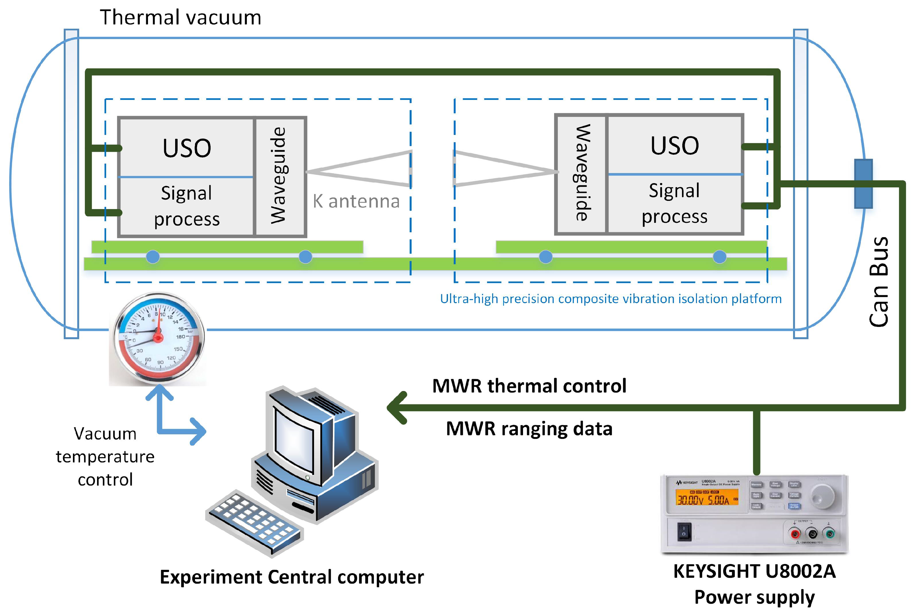
4.1. Laboratory Experiment Environment

The proposed thermal control system was extensively tested in a laboratory environment on the ground, before launch. The relevant metal materials and heating parameters of MWR thermal test are given in

Table 1. Metal materials and heating/cooling parameters of MWR thermal test.

Payload	Materials 1	Heat Capacity (J/kg·K)	Block mass (kg)	Thermal conductivity (W/m·K)	Heating Patch Surface Area (mm × mm)	Nominal Heat/Cool Power (W)	Saturation Heat/Cool Power (W)
antenna	magaluma 5086	9.00 × 10${}^2$	1.45	127	50 × 20	8	3.5
waveguide	nickel alloy GH4169	6.15 × 10${}^2$	0.50	23.6	20 × 10	4	3.5
signal process	aluminum alloy AZ91D	8.80 × 10${}^2$	2.14	51	80 × 30	8	3.5
USO	aluminum alloy AZ91D	8.80 × 10${}^2$	0.67	51	60 × 30	5	3.5

¹ Manufacturing major metal materials.

as:

Parameters for the nominal PID control in Equation (2) include $K_p=40$, $K_I=0.5$, $K_D=5$, and sampling time is $T_s=5s$. According to the massive experiments, the thermal dynamic model is:

$$\dot{\mathit{x}}\left(t\right)=\left[\begin{array}{cccc}{\mathit{A}}_{11}& {\mathit{A}}_{12}& {\mathit{A}}_{13}& {\mathit{A}}_{14}\\ \mathbf{0}& {\mathit{A}}_{22}& {\mathit{A}}_{23}& {\mathit{A}}_{24}\\ \mathbf{0}& \mathbf{0}& {\mathit{A}}_{33}& {\mathit{A}}_{34}\\ \mathbf{0}& \mathbf{0}& \mathbf{0}& {\mathit{A}}_{44}\end{array}\right]\mathit{x}\left(t\right)+\left[\begin{array}{cccc}{\mathit{B}}_{11}& {\mathit{B}}_{12}& {\mathit{B}}_{13}& {\mathit{B}}_{14}\\ \mathbf{0}& {\mathit{B}}_{22}& {\mathit{B}}_{23}& {\mathit{B}}_{24}\\ \mathbf{0}& \mathbf{0}& {\mathit{B}}_{33}& {\mathit{B}}_{34}\\ \mathbf{0}& \mathbf{0}& \mathbf{0}& {\mathit{B}}_{44}\end{array}\right]\sigma \left(\mathit{u}\left(t\right)\right)$$

(43)

Detailed information of the submatrix can be found in Appendix A.

The overall thermal control experiment system for the MWR time-delay test was carefully designed to provide a temperature control environment with precision, high stability, and a wide range of output, with a vibration isolation environment that had a vibration amplitude of less than 1 µm. The schematic diagram of the whole test system is given in Figure 4 below.

The whole thermal control system includes precise controllable temperature and humidity thermal vacuum equipment, ultra-high precision composite vibration isolation platform, MWR payload, MWR data sampling, and a process system and power supply, as shown in Figure 4. The MWR microwave ranging system A and B were placed on the vibration isolation platform with the thermal insulation structure, reducing the temperature of the isolation platform, affecting the measured MWR equipment. The data acquisition and processing system, power supply, etc., were placed on the laboratory desktop to avoid other heat sources, vibration, etc., from affecting the tested payload.

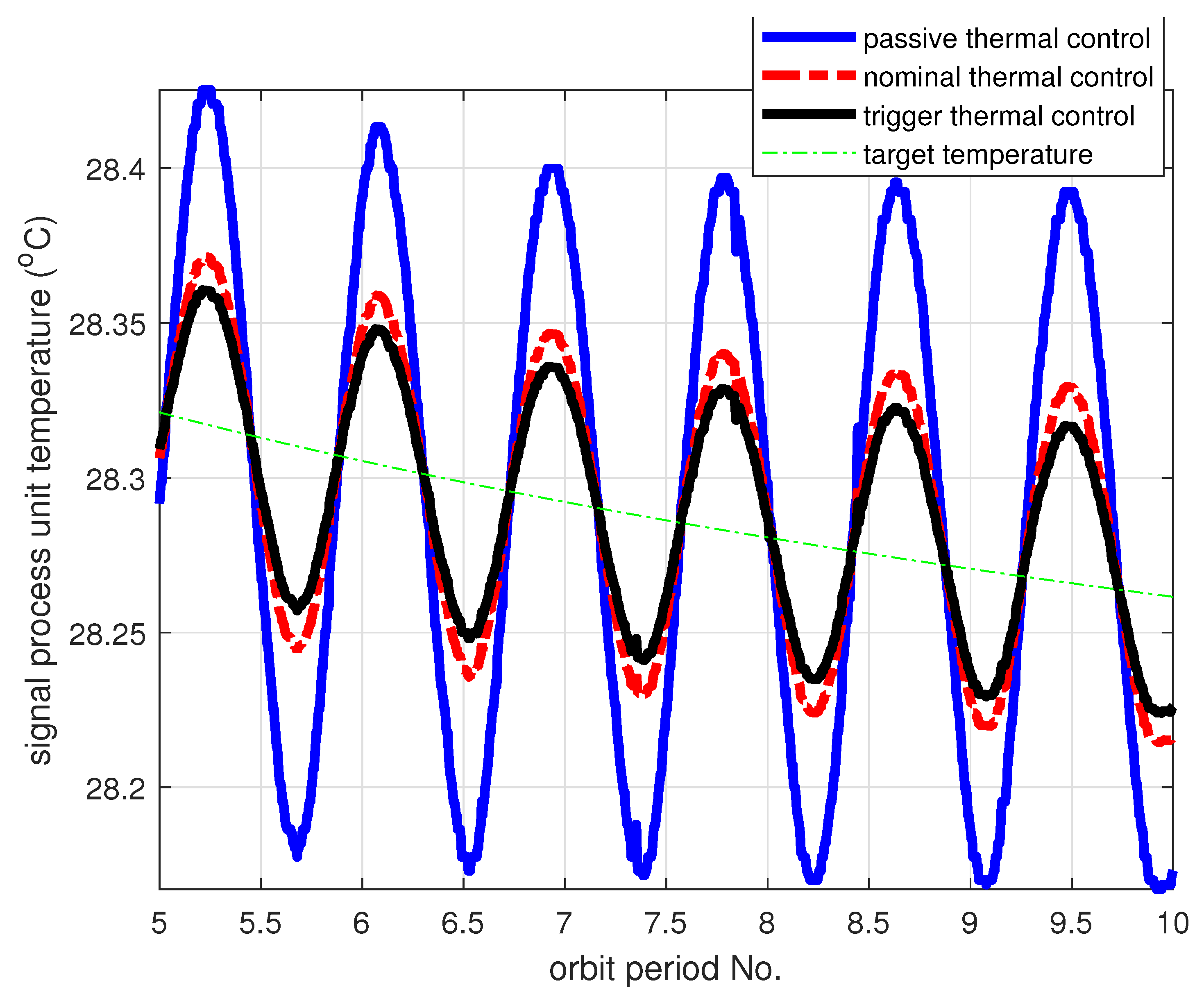
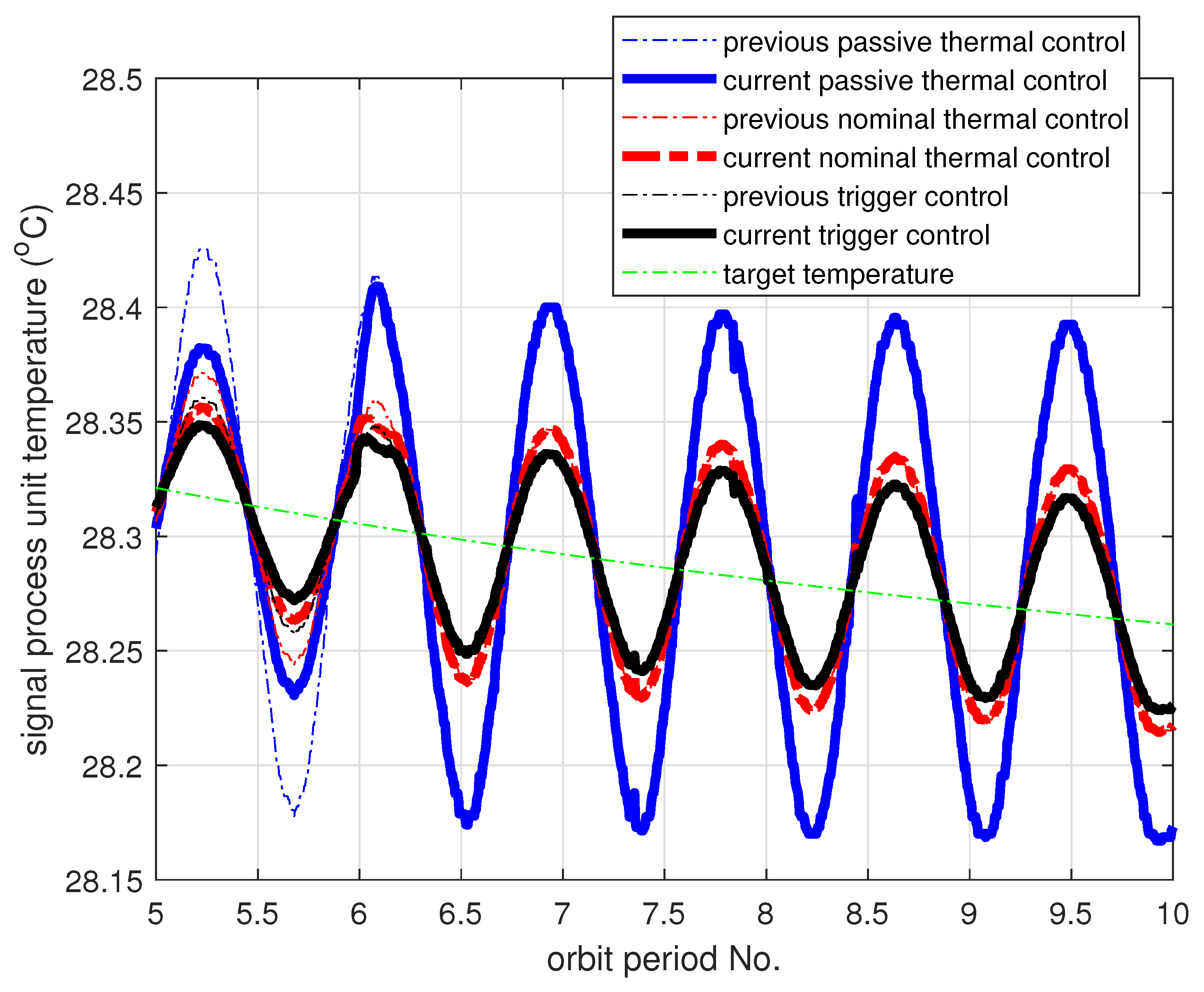
4.2. Performance of Passive and Nominal Thermal Control

To fully simulate the on-orbit thermal condition of the internal satellite compartment, we provide the baseline follow-on formation mission as: Chief spacecraft orbit altitude: 500 km; inclination: 89.2 deg; argument of perigee: 0 deg; RAAN: 0 deg; true anomaly: 0 deg; the deputy spacecraft followed the in-line flight relative to the chief spacecraft, with a distance of about 180 km in-track [57].

The bold blue lines in Figure 5 show the measured temperature of the ranging payloads inside the thermal vacuum equipment without active control, from sampled data during the experiment. Note that there are four sensors around each payload; the results in Figure 5 demonstrate the average temperature of those four sensors for each payload. For the sake of clarity, here we just provide the thermal states after temperature convergence from the fifth to tenth orbit. The results represent the satellite internal ranging payload thermal condition during the formation scene on-orbit, which mostly exhibit periodic fluctuations.

Clearly, the passive thermal protection method performed stably during the on-orbit mission time, about ±0.15 ${}^{\circ }$C when convergence occurred, which verified our model for practical use in a real space mission; however, for more precision ranging performance, it is necessary to conduct active thermal control to achieve less temperature fluctuations. The thermal experiment was conducted again with the same parameters. The green lines in Figure 5 are the target temperatures of each payload, through online curve fitting, and the bold dotted red lines show the results of the nominal thermal PID control as introduced in Section 2.2. The results show the decreased temperature fluctuation of about ±0.1 ${}^{\circ }$C, compared with passive thermal control.

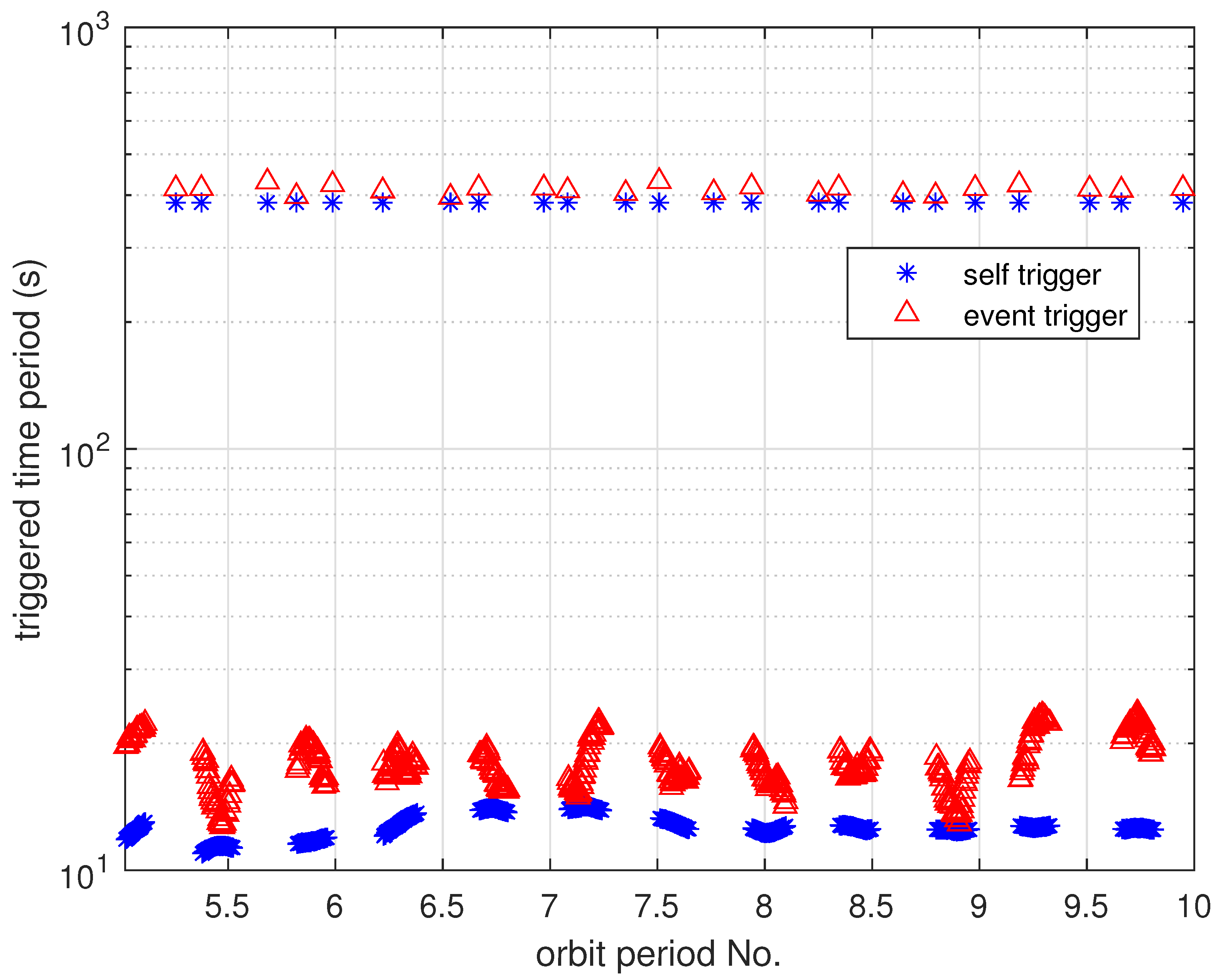
4.3. Performance of Trigger Control

The performance of proposed trigger control was tested, and is described in this section. Here, we set the parameters of $\gamma =0.5, \delta =0.02$, meaning the triggered threshold value from the measured states. Saturation control $\overline{\mathit{u}}$ complied with the data from Table 1 for each payload, and $\mathit{S}=\mathit{D}=diag\left[0.15I_{4\times 4}0.1I_{4\times 4}0.15I_{4\times 4}0.1I_{4\times 4}\right]$ in Equation (11).

Figure 6 provides the experimental results of the self-triggered control for the signal process unit payload. We obtained less temperature fluctuation results (bold solid black line) compared to the nominal control. The reason for this improvement is due to the adopted optimal control that minimized the difference of nominal thermal trajectory to the target ones. The other payloads obtained similar thermal control performance as the signal process unit, which is not shown here for the sake of brevity.

It is interesting to find the internal states by using triggered control; Figure 7 shows the triggered sample periods of the signal process unit payload. Clearly, the triggered control system design can effectively adjust the sampling period, compared to the nominal PID control of the fixed sampling time, according to the error state perturbations. Moreover, the event-trigger (red triangle) could reduce the sampling period frequency better than the self-triggered (blue stars) approach during our experiments—about 60–120 s for event-trigger and 20–35 s for self-trigger—during the undersaturation actuator stages. The reason for this phenomenon is that the event-trigger uses external thermal sensors to obtain state updates, and the self-trigger uses model prediction state information, which increased the sampling frequency more than the event-trigger structure. The upper data in Figure 7 show that the trigger points in the control saturation begin/end stages and regional minimum/maximum temperatures.

4.4. Performance of Learning Process

The thermal control system modeling may differ from the original design as a space mission lasts for years. Here, we use the proposed online learning method for the thermal system with the following parameters: positive semidefinite matrix $\mathit{M}$ and positive definite matrix $\mathit{R}$

$$\mathit{M}=\mathrm{diag}\left[\begin{array}{cccc}{10}^{-8}& {10}^{-8}& {10}^{-9}& {10}^{-9}\end{array}\right],\mathit{R}=\mathrm{diag}\left[\begin{array}{cccc}{10}^{-5}& {10}^{-5}& {10}^{-5}& {10}^{-5}\end{array}\right]$$

the actor/critic approximator constant gain ${\alpha }_a=0.1$, ${\alpha }_c=50$ in Equations (39) and (40). Moreover, a 0.5 kg aluminum alloy block is patched closely with the signal process unit, until the end of the 6th orbit period, simulating the thermal system model uncertainty in space. For the experiments during orbit No. 0–6, an exploration noise was added in the control input along with nominal one to ensure persistence of excitation and state exploration.

Figure 8 shows the performance of the thermal control system with the learning process for the signal process unit payload. The results of previous and current experiments are clearly marked as thin lines and bold lines, respectively, and compared to Figure 6. It is interesting to find that the thermal system gradually recovered to normal states since the beginning of orbit No.6, as the aluminum alloy block separated from the payload and the nominal/trigger control trajectory experienced a tracking process, marked as bold red/black lines. The results illustrate the efficacy of the proposed learning algorithm when the system model was disturbed with unknown information, which can be adaptively converged to stable states. Moreover, it is meaningful to find that the internal thermal condition can be improved if a big metal alloy block is used.

4.5. Time-Delay Performance of MWR Ranging System

The time-delay (ranging error) fluctuation performance of the microwave ranging system is closely related to the thermal stability of each payload on-orbit. The active microwave payloads used in the experiment were carefully tested separately at a precisely controlled constant temperature and humidity cleaning platform in advance, which revealed the time-delay coefficient (TDC—meaning the time delay value per degree Celsius) of 40 µm/K, 48 µm/K for K-band antenna and waveguide switch network; 19 µm/K, 25 µm/K for the signal process unit and USO [57]. Moreover, the time delay of the whole K-band ranging system can be realized as less than 5 µm if the payload thermal system is well protected within about 0.1 ${}^{\circ }$C fluctuation.

The final microwave ranging error using the proposed trigger-based thermal control structure design is shown in Figure 9 with a black line. Clearly, the thermal control system performed stably after convergence by using the optimal online triggered control structure. The ranging accuracy with passive thermal control can achieve less than approximately 6 µm in orbit No.10 (max-min) and less than 3.5 µm by using nominal thermal control. The 25% (RMS) accuracy improvement can be realized by using the trigger-based control strategy, about 2.2 µm from the test, compared to the nominal control method.

5. Discussion

Aiming to improve autonomous and accuracy MWR ranging performance in real space missions, this paper proposed a trigger-based payload thermal control system design with an online learning process. The whole structure can be selected through option switch, according to actual needs. Basically, a nominal controller is used for coarse control under a new thermal environment, and can be switched to a trigger-based controller during the mission, minimizing the communication resources required from the spacecraft platform. RL-based control is suitable for long-term missions in space, particularly in cases where thermodynamic conditions deteriorate. The computational complexity is increased as we introduced the nominal control, trigger-based control (in trigger condition computation), and RL-based control (in actor/critic approximation iteration steps). The performance of the proposed trigger thermal control system is verified in a laboratory, which demonstrated the efficiency in communication reduction and temperature stability to practical use. The effectiveness of learning process was also validated under conditions of thermal dynamic modeling uncertainty. Finally, the ranging accuracy was tested for the whole payload system; we found that a 25% (RMS) performance improvement can be realized by using a trigger-based control strategy, about 2.2 µm compared to the nominal control method.

References

1. Landerer, F.W.; Flechtner, F.M.; Save, H.; Webb, F.H.; Bandikova, T.; Bertiger, W.I.; Bettadpur, S.V.; Byun, S.H.; Dahle, C.; Dobslaw, H.; et al. Extending the global mass change data record: GRACE Follow-On instrument and science data performance. Geophys. Res. Lett. 2020, 47, e2020GL088306. [Google Scholar] [CrossRef]
2. Bryant, R.; Moran, M.S.; McElroy, S.A.; Holifield, C.; Thome, K.J.; Miura, T.; Biggar, S.F. Data continuity of Earth observing 1 (EO-1) Advanced Land I satellite image (ALI) and Landsat TM and ETM+. IEEE Trans. Geosci. Remote Sens. 2003, 41, 1204–1214. [Google Scholar] [CrossRef]
3. Totani, T.; Ogawa, H.; Inoue, R.; Das, T.K.; Wakita, M.; Nagata, H. Thermal design procedure for micro- and nanosatellite pointing to earth. J. Thermophys. Heat Transf. 2014, 28, 524–533. [Google Scholar] [CrossRef]
4. Reiss, P.; Hager, P.; Bewick, C. New methodologies for the thermal modeling of CubeSats. In Proceedings of the 26th Annual AIAA/USU Conference on Small Satellites, Logan, UT, USA, 13–16 August 2012; pp. 1–12. [Google Scholar]
5. Jiang, X.; Han, Q.L.; Liu, S.; Xue, A. A New H Stabilization Criterion for Networked Control Systems. IEEE Trans. Autom. Control 2008, 53, 1025–1032. [Google Scholar] [CrossRef]
6. Astrom, K.J.; Bernhardsson, B.M. Comparison of Riemann and Lebesgue sampling for first order stochastic systems. In Proceedings of the 41st IEEE Conference on Decision and Control, Las Vegas, NV, USA, 10–13 December 2002; Volume 2, pp. 2011–2016. [Google Scholar]
7. Pan, H.; Chang, X.; Zhang, D. Event-triggered adaptive control for uncertain constrained nonlinear systems with its application. IEEE Trans. Ind. Inform. 2019, 16, 3818–3827. [Google Scholar] [CrossRef]
8. Liu, W.; Huang, J. Event-triggered global robust output regulation for a class of nonlinear systems. IEEE Trans. Autom. Control 2017, 62, 5923–5930. [Google Scholar] [CrossRef]
9. Xing, L.; Wen, C.; Liu, Z.; Su, H.; Cai, J. Event-Triggered Output Feedback Control A Cl. Uncertain Nonlinear Systems. IEEE Trans. Autom. Control 2018, 64, 290–297. [Google Scholar] [CrossRef]
10. Wang, R.; Si, C.; Ma, H.; Hao, C. Global event-triggered inner-outer loop stabilization of under-actuated surface vessels. Ocean Eng. 2020, 218, 108228. [Google Scholar] [CrossRef]
11. Zhang, J.; Liu, S.; Liu, J.F. Economic model predictive control with triggered evaluations: State and output feedback. J. Process Control 2014, 24, 1197–1206. [Google Scholar] [CrossRef]
12. Shahid, M.I.; Ling, Q. Event-triggered distributed dynamic output-feedback dissipative control of multi-weighted and multi-delayed large-scale systems. ISA Trans. 2020, 96, 116–131. [Google Scholar] [CrossRef]
13. Azimi, M.M.; Afzalian, A.A.; Ghaderi, R. Decentralized stabilization of a class of large scale networked control systems based on modified event-triggered scheme. Int. J. Dyn. Control 2021, 9, 149–159. [Google Scholar] [CrossRef]
14. Li, F.; Cao, X.; Zhou, C.; Yang, C. Event-triggered asynchronous sliding mode control of CSTR based on Markov Model. J. Frankl. Inst. 2021, 358, 4688–4704. [Google Scholar] [CrossRef]
15. Wang, W.; Tong, S. Distributed adaptive fuzzy event-triggered containment control of nonlinear strict-feedback systems. IEEE Trans. Cybern. 2019, 50, 3973–3983. [Google Scholar] [CrossRef] [PubMed]
16. Su, X.; Liu, Z.; Lai, G.; Zhang, Y.; Chen, C.P. Event-triggered adaptive fuzzy control for uncertain strict-feedback nonlinear systems with guaranteed transient performance. IEEE Trans. Fuzzy Syst. 2019, 27, 2327–2337. [Google Scholar] [CrossRef]
17. Abhinav, S.; Rajiv, K.M. Control of a nonlinear continuous stirred tank reactor via event triggered sliding modes. Chem. Eng. Sci. 2018, 187, 52–59. [Google Scholar]
18. Tang, X.T.; Deng, L. Multi-step output feedback predictive control for uncertain discrete-time T-S fuzzy system via event-triggered scheme. Automatica 2019, 107, 362–370. [Google Scholar] [CrossRef]
19. Li, S.; Ahn, C.K.; Guo, J.; Xiang, Z. Neural-Network Approximation-Based Adaptive Periodic Event-Triggered Output-Feedback Control of Switched Nonlinear Systems. IEEE Trans. Cybern. 2020, 51, 4011–4020. [Google Scholar] [CrossRef]
20. Liu, D.; Yang, G.H. Neural Network-Based Event-Triggered MFAC for Nonlinear Discrete-Time Processes. Neurocomputing 2018, 272, 356–364. [Google Scholar] [CrossRef]
21. Xing, X.; Liu, J. Event-triggered neural network control for a class of uncertain nonlinear systems with input quantization. Neurocomputing 2021, 440, 240–250. [Google Scholar] [CrossRef]
22. Yang, X.; Wei, Q.L. Adaptive Critic Designs for Optimal Event-Driven Control of a CSTR System. IEEE Trans. Ind. Inform. 2020, 17, 484–493. [Google Scholar] [CrossRef]
23. Yang, X.; He, H. Event-Driven H∞-Constrained Control Using Adaptive Critic Learning. IEEE Trans. Cybern. 2020, 51, 4860–4872. [Google Scholar] [CrossRef] [PubMed]
24. Yang, X.; Zhu, Y.; Dong, N.; Wei, Q.L. Decentralized Event-Driven Constrained Control Using Adaptive Critic Designs. IEEE Trans. Neural Netw. Learn. Syst. 2021; 1–15, Early Access. [Google Scholar] [CrossRef] [PubMed]
25. Seuret, A.; Prieur, C.; Tarbouriech, S.; Zaccarian, L. Event-triggered control with LQ optimality guarantees for saturated linear systems. IFAC Proc. Vol. 2013, 46, 341–346. [Google Scholar] [CrossRef] [Green Version]
26. Tarbouriech, S.; Garcia, G.; da Silva, J.M.G., Jr.; Queinnec, I. Stability and Stabilization of Linear Systems with Saturating Actuators; Springer Science & Business Media: Berlin, Germany, 2011. [Google Scholar]
27. Wu, W.; Reimann, S.; Liu, S. Event-triggered control for linear systems subject to actuator saturation. IFAC Proc. Vol. 2014, 47, 9492–9497. [Google Scholar] [CrossRef] [Green Version]
28. Åarzén, K.E. A simple event-based PID controller. IFAC Proc. Vol. 1999, 32, 8687–8692. [Google Scholar] [CrossRef]
29. Heemels, W.P.; Gorter, R.J.; Van Zijl, A.; Van den Bosch, P.P.; Weiland, S.; Hendrix, W.H.; Vonder, M.R. Asynchronous measurement and control: A case study on motor synchronization. Control Eng. Pract. 1999, 7, 1467–1482. [Google Scholar] [CrossRef]
30. Velasco, M.; Fuertes, J.; Marti, P. The self triggered task model for real-time control systems. In Proceedings of the Work-in-Progress Session of the 24th IEEE Real-Time Systems Symposium (RTSS03), Cancun, Mexico, 3–5 December 2003; Volume 384, pp. 67–70. [Google Scholar]
31. Heemels, W.; Johansson, K.H.; Tabuada, P. An introduction to event-triggered and self-triggered control. In Proceedings of the 2012 IEEE 51st IEEE Conference on Decision and Control (CDC), Maui, HI, USA, 10–13 December 2012; pp. 3270–3285. [Google Scholar]
32. Yi, X.; Liu, K.; Dimarogonas, D.V.; Johansson, K.H. Dynamic event-triggered and self-triggered control for multi-agent systems. IEEE Trans. Autom. Control 2018, 64, 3300–3307. [Google Scholar] [CrossRef]
33. Wang, X.; Lemmon, M.D. Self-Triggered Feedback Control Systems with Finite-Gain L2 Stability. IEEE Trans. Autom. Control 2009, 54, 452–467. [Google Scholar] [CrossRef]
34. Almeida, J.; Silvestre, C.; Pascoal, A.M. Self-triggered state-feedback control of linear plants under bounded disturbances. Int. J. Robust Nonlinear Control 2015, 25, 1230–1246. [Google Scholar] [CrossRef]
35. Peng, C.; Han, Q.L. On designing a novel self-triggered sampling scheme for networked control systems with data losses and communication delays. IEEE Trans. Ind. Electron. 2015, 63, 1239–1248. [Google Scholar] [CrossRef]
36. Buşoniu, L.; de Bruin, T.; Tolić, D.; Kober, J.; Palunko, I. Reinforcement learning for control: Performance, stability, and deep approximators. Annu. Rev. Control 2018, 46, 8–28. [Google Scholar] [CrossRef]
37. Vamvoudakis, K.G. Q-learning for continuous-time linear systems: A model-free infinite horizon optimal control approach. Syst. Control Lett. 2017, 100, 14–20. [Google Scholar] [CrossRef]
38. Fortunato, M.; Azar, M.G.; Piot, B.; Menick, J.; Osband, I.; Graves, A.; Mnih, V.; Munos, R.; Hassabis, D.; Pietquin, O.; et al. Noisy networks for exploration. arXiv 2017, arXiv:1706.10295. [Google Scholar]
39. Asadi, K.; Littman, M.L. An alternative softmax operator for reinforcement learning. In Proceedings of the International Conference on Machine Learning, Sydney, NSW, Australia, 6–11 August 2017; PMLR 2017. pp. 243–252. [Google Scholar]
40. Engel, Y.; Mannor, S.; Meir, R. Reinforcement learning with Gaussian processes. In Proceedings of the 22nd International Conference on Machine Learning, Bonn, Germany, 7–11 August 2005; pp. 201–208. [Google Scholar]
41. Sutton, R.S.; McAllester, D.; Singh, S.; Mansour, Y. Policy gradient methods for reinforcement learning with function approximation. Adv. Neural Inf. Process. Syst. 2000, 12, 1057–1063. [Google Scholar]
42. Jha, S.K.; Roy, S.B.; Bhasin, S. Direct adaptive optimal control for uncertain continuous-time LTI systems without persistence of excitation. IEEE Trans. Circuits Syst. II Express Briefs 2018, 65, 1993–1997. [Google Scholar] [CrossRef]
43. Tu, S.; Recht, B. Least-squares temporal difference learning for the linear quadratic regulator. In Proceedings of the International Conference on Machine Learning, Stockholm, Sweden, 10–15 July 2018; PMLR 2018. pp. 5005–5014. [Google Scholar]
44. Umenberger, J.; Schön, T.B. Learning convex bounds for linear quadratic control policy synthesis. Adv. Neural Inf. Process. Syst. 2018, 31. Available online: https://proceedings.neurips.cc/paper/2018/hash/f610a13de080fb8df6cf972fc01ad93f-Abstract.html (accessed on 3 July 2022).
45. Lee, D.; Hu, J. Primal-dual Q-learning framework for LQR design. IEEE Trans. Autom. Control 2018, 64, 3756–3763. [Google Scholar] [CrossRef]
46. Konda, V.R.; Tsitsiklis, J.N. On actor-critic algorithms. SIAM J. Control Optim. 2003, 42, 1143–1166. [Google Scholar] [CrossRef]
47. Lee, D.; Lin, C.J.; Lai, C.W.; Huang, T. Smart-valve-assisted model-free predictive control system for chiller plants. Energy Build. 2021, 234, 110708. [Google Scholar] [CrossRef]
48. Qiu, S.; Li, Z.; Fan, D.; He, R.; Dai, X.; Li, Z. Chilled water temperature resetting using model-free reinforcement learning: Engineering application. Energy Build. 2022, 255, 111694. [Google Scholar] [CrossRef]
49. Wang, X.; Gong, D.; Jiang, Y.; Mo, Q.; Kang, Z.; Shen, Q.; Wu, S.; Wang, D. A Submillimeter-Level Relative Navigation Technology for Spacecraft Formation Flying in Highly Elliptical Orbit. Sensors 2020, 20, 6524. [Google Scholar] [CrossRef] [PubMed]
50. Wang, X.; Wu, S.; Gong, D.; Shen, Q.; Wang, D.; Damaren, C. Evaluation of Precise Microwave Ranging Technology for Low Earth Orbit Formation Missions with Beidou Time-Synchronize Receiver. Sensors 2021, 21, 4883. [Google Scholar] [CrossRef]
51. Min, G. Satellite Thermal Control Technology; China Astronautics Press: Beijing, China, 1991; Volume 249. (In Chinese) [Google Scholar]
52. Choi, M. Thermal assessment of swift instrument module thermal control system and mini heater controllers after 5+ Years in Flight. In Proceedings of the 40th International Conference on Environmental Systems, Barcelona, Spain, 11–15 July 2010. AAAA 2010-6003. [Google Scholar]
53. Choi, M. Thermal Evaluation of NASA/Goddard Heater Controllers on Swift BAT, Optical Bench and ACS. In Proceedings of the 3rd International Energy Conversion Engineering Conference, San Francisco, CA, USA, 15–18 August 2005. AAAA 2005-5607. [Google Scholar]
54. Granger, J.; Franklin, B.; Michalik, M.; Yates, P.; Peterson, E.; Borders, J. Fault-Tolerant, Multiple-Zone Temperature Control; NASA Tech Briefs: New York, NY, USA, 1 September 2008; No. NPO-45230.
55. Lewis, F.L.; Syrmos, V. Optimal Control; Wiley: New York, NY, USA, 1995. [Google Scholar]
56. Bradtke, S.J.; Barto, A.G. Linear least-squares algorithms for temporal difference learning. Mach. Learn. 1996, 22, 33–57. [Google Scholar] [CrossRef] [Green Version]
57. Jiao, Z.; Wang, D.; Liu, X.; Ren, S.; Yang, S.; Zhong, X. Test and research on time delay stability of micron microwave ranging system. Space Electron. Technol. 2021, 18, 58–63. (In Chinese) [Google Scholar]
Figure 1. Structure of the satellite: (a) K-band antenna phase center; (b) K-band microwave ranging system payload; (c) centroid adjustment; (d) accelerometer for gravity field detection; (e) star sensor; (f) power supply; (g) fuel tank; (h) thruster.
Electronics 11 02173 g001
Figure 2. Structure of the trigger-based thermal control system.
Electronics 11 02173 g002
Figure 3. Structure of the triggered thermal control system with learning process.
Electronics 11 02173 g003
Figure 4. Schematic diagram of the MWR thermal control system in laboratory environment.
Electronics 11 02173 g004
Figure 5. The thermal states of K-band MWR payloads during test. (a) K-band antenna; (b) waveguide switch network; (c) signal process unit; (d) USO.
Electronics 11 02173 g005
Figure 6. Comparison of different thermal control algorithms for signal process unit.
Electronics 11 02173 g006
Figure 7. Sample period vs. orbit number for self-/event-triggered control.
Electronics 11 02173 g007
Figure 8. Comparison of different thermal control algorithms with learning processes for the signal process unit.
Electronics 11 02173 g008
Figure 9. The micron level ranging error during different thermal control processes.
Electronics 11 02173 g009