Joint Inversion of Evaporation Duct Based on Radar Sea Clutter and Target Echo Using Deep Learning

Abstract

Tropospheric duct is an anomalous atmospheric phenomenon over the sea surface that seriously affects the normal operation and performance evaluation of electromagnetic communication equipment at sea. Therefore, achieving precise sensing of tropospheric duct is of profound significance for the propagation of electromagnetic signals. The approach of inverting atmospheric refractivity from easily measurable radar sea clutter is also known as the refractivity from clutter (RFC) technique. However, inversion precision of the conventional RFC technique is low in the low-altitude evaporation duct environment. Due to the weak attenuation of the over-the-horizon target signal as it passes through the tropospheric duct, its strength is much stronger than that of sea clutter. Therefore, this study proposes a new method for the joint inversion of evaporation duct height (EDH) based on sea clutter and target echo by combining deep learning. By testing the inversion performance and noise immunity of the new joint inversion method, the experimental results show that the mean error RMSE and MAE of the new method proposed in this paper are reduced by 41.2% and 40.3%, respectively, compared with the conventional method in the EDH range from 0 to 40 m. In particular, the RMSE and MAE in the EDH range from 0 to 16.7 m are reduced by 54.2% and 56.4%, respectively, compared with the conventional method. It shows that the target signal is more sensitive to the lower evaporation duct, which obviously enhances the inversion precision of the lower evaporation duct and has effectively improved the weak practicality of the conventional RFC technique.

1. Introduction

The marine atmospheric boundary layer (MABL) is a dynamic area in the lower troposphere over the sea surface, which directly interacts with the marine environment through energy, momentum and material exchange, and has a tremendous effect on the weather and climate in local areas and even globally [1]. The MABL frequently occurs when temperature and humidity are distributed abnormally across the vertical gradient, and this abnormal environment can affect the atmospheric refractivity, which will influence the propagation path and attenuation features of electromagnetic waves in the atmosphere [2]. This type of phenomenon, which is called tropospheric duct, causes electromagnetic waves to be trapped within it, affecting the electromagnetic wave distribution in the area above the duct layer, and creating unexpected voids and target identification errors, to affect radar performance [3]. The main effects of tropospheric duct on radar performance are shown in Figure 1.

Evaporation duct is the commonest type of tropospheric duct, which often occurs in the near sea surface atmosphere below 40 m height and is composed of a shallow trap layer [4,5,6]. In addition, the occurrence probability of evaporation duct and evaporation duct height (EDH) varies obviously with the geographical area, season and time of day. Usually, the probability of evaporation duct occurrence is higher and EDH is higher during summer and daytime in low-latitude seas.

Currently, there are disadvantages such as high cost and poor data collection when using equipment to directly measure atmospheric refractivity for tropospheric duct [7]. Considering that tropospheric duct can obviously affect the sea surface scattering signal of radar, in the 1990s, the US Naval Surface Warfare Center proposed a technique referred to as refractivity from clutter (RFC). The RFC technique can invert the atmospheric refractivity without using additional detection equipment, simply using the sea clutter data obtained during the routine operation of radar, combined with an effective inversion algorithm. Later, an experiment (called Wallops98) was performed to invert refractivity of tropospheric duct from radar clutter, whose results show the feasibility and efficiency of the RFC technique. For numerous important applications of tropospheric duct, recently, research on refractivity features in MABL is primarily focused on the application and optimization of RFC [8,9].

In 1999, Rogers et al. [10] inverted the EDH using a least squares optimization method. In 2001, Vasudevan et al. [11] modeled the inversion problem as a parameter estimation problem in a nonlinear state space and carried out the solution using the serial importance sampling (SIS) method. In 2003, Gerstoft et al. [12] modeled the inversion problem as a global optimization problem, and applied simulated annealing (SA) and genetic algorithms (GA) together with the RFC technique to invert the atmospheric refractivity from radar clutter. In 2004, Barrios [13] used the moment technique to invert the modified refractivity profile of surface based duct based on ray density and radar clutter data. In 2006, Yardim et al. [14] used the markov chain monte carlo (MCMC) sampling technique to sample the vector space of the profile parameters and calculated the posterior probability density distribution of the profile parameters by Bayesian theory. In 2007, Yardim et al. [15] proposed a hybrid GA-MCMC algorithm for fast calculation of the posterior probability distribution of the refractivity profile.

With the development of varied optimization algorithms, machine learning algorithms are widely used in the study of inverting atmospheric refractivity. And as the requirement for inversion precision increases, the disadvantages of shallow machine learning, such as simple structure and weak learning ability, gradually appear. In recent years, there are increasing numbers of scholars focusing on deep learning with unique structural features [16]. In 2018, Guo et al. [17] calculated the sea clutter power in different duct environments based on sea clutter calculation theory and used deep neural networks (DNN) to invert the refractivity profile parameters of evaporation duct and surface based duct.

Using a more refined inversion model necessarily makes the inversion more difficult. In addition to the model required for the inversion, the information amount of the inversion input also greatly affects the precision of the inversion. Joint inversion is an important technique for the geophysical industry in order to conduct quantitative studies, and plays a major role in geological exploration and other fields [18]. In 1991, Alekseev [19] set out in detail the method of solving the joint inversion problem and the general features of the solution, giving a preliminary theoretical conclusion that joint inversion is superior to using one kind of observed data. After continuous development and evolution, some scholars proposed an inversion method using different kinds of observations, and this inversion method is seen as the inevitable trend and the best choice for joint inversion [20]. In the last decade, many scholars have proposed various improvements based on the joint inversion method to enhance the inversion precision for the RFC technique [21,22,23,24].

Since the scattered echo from the sea surface target contains not only the location, velocity, and size of the detection target, but also many important information about the environmental conditions of the tropospheric duct can be also detected, and the strength of the received target signal is much stronger than that of the sea clutter [25]. Therefore, the refractivity profile parameters in the tropospheric duct environment can be inverted jointly by using radar sea clutter and over-the-horizon target echo, and increasing the data of the target echo signal can be regarded as increasing the information capacity of the inversion, which can theoretically enhance the precision of the inversion.

The novelty of this paper is as follows. To solve the limitations of low inversion precision and weak practicability for the conventional inversion model, on the basis of deep learning, we introduce the over-the-horizon target signal with strong strength and propose a new joint inversion method based on sea clutter and target echo, focusing on the low-altitude evaporation duct environment over the sea surface. To thoroughly verify the comprehensive performance of the joint inversion model, we use the conventional method as the experimental baseline model. Then, we extensively test the general performance of the joint inversion model through comparison of inversion performance and the noise immunity test. Experimental results show that the performance of the new deep learning joint inversion method is superior to that of the conventional inversion method. The new method considers the effect of evaporation duct on both sea clutter and over-the-horizon target signals, so it overcomes the problem that the inversion precision of low altitude duct is very low when using only sea clutter.

2. Evaporation Duct Refractivity Profile, Sea Clutter Power and Target Echo Power Calculation

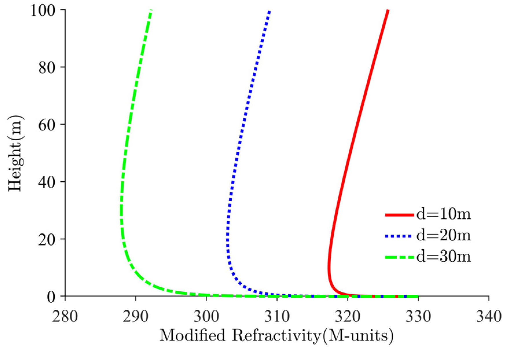
2.1. Evaporation Duct Refractivity Profile Model

Atmospheric refractivity features in evaporation duct environments are still a research hot spot and a challenge, because the probability of evaporation duct occurring is far higher than that of other types of duct. A series of models for calculating the refractivity profile of evaporation duct, such as the Paulus-Jeske (P-J) model, the Musson-Genon-Gauthier-Burth (MGB) model and the Babin model, have been established based on the Monin-Obukhov similarity theory of the atmospheric boundary layer, which has been studied more intensively abroad [26].

The evaporation duct refractivity profile model in this study was originally proposed by Jeske in 1973. Subsequently, Paulus found that using the Jeske model would result in higher predicted EDHs than the actual values because of the effect that land would have on the measurement of near-coastal atmospheric temperatures. Paulus performed a specialized correction to the Jeske model and proposed the P-J model [27]. The modified reflectivity profiles for different EDHs are shown in Figure 2. Based on the relationship between the atmospheric refractivity and various atmospheric factors, the modified P-J model can be modeled as a log-linear formula for the height:

$$M(z)=M(0)+0.125z-0.125d\ln (\frac{z+z_0}{z_0})$$

(1)

where, d is the EDH in meters, which is an important feature parameter of the evaporation duct refractivity profile. z is the height on the sea surface in meters, and $z_0$ is the aerodynamic surface roughness of the marine, which generally takes the value of $1.5\times {10}^{-4}$ m. $M_0$ is the modified refractivity on the sea surface, and its typical value is 330.

From the P-J model, the refractivity profile of the evaporation duct can be obtained by knowing the height parameter of the evaporation duct. The inversion of the evaporation duct is converted into the inversion of the refractivity profile parameter. Thus, it decreases the complexity of the inversion and enhances the feasibility of inversion.

2.2. Target Echo and Sea Clutter Power Calculation

When a radar detects a target on sea surface, a portion of the signal that is re-radiated to the radar is called back scattering [28,29]. This back scattering is the target echo signal received by the radar. According to the radar equation, assuming that the range between the radar receiving antenna and the target with an effective radar cross section (RCS) of $\sigma$ is r [30], the signal power received by the radar can be expressed as:

$$P_s=\frac{4\pi P_t{G}_t{G}_r\sigma }{L^2{\lambda }^2}$$

(2)

where $P_t$ is the transmitter power, and $P_t$ and $G_t$ are the gains of the transmitting and receiving antennas, respectively. $\lambda$ is the wavelength, $\sigma$ is the RCS of the target, and L is the loss in the propagation of electromagnetic waves. In general, the propagation loss L arising from the propagation of electromagnetic waves in tropospheric duct can be expressed as:

$$L=32.45+20\lg f+20\lg r-20\lg F$$

(3)

where f is frequency, and F represents the propagation factor. The propagation factor takes into account the influence of the atmospheric refractivity in the tropospheric duct and the parameters of the radar system on the propagation of electromagnetic waves. According to the definition of field strength, F can be expressed as:

$$F=\sqrt{x}\left|u(x,z)\right|$$

(4)

where $u(x,z)$ is the component of the field strength in the vertical and horizontal directions. We can use the parabolic equation (PE) method to model the $u(x,z)$. The final form of the PE used in this study can be expressed as:

$$\frac{{\partial }^{2}u(x,z)}{\partial z^2}+2ik\frac{\partial u(x,z)}{\partial z}+k^2(n^2(x,z)-1)u(x,z)=0$$

(5)

where k is the number of electromagnetic waves, and n is the atmospheric refractivity index. We can solve the PE by the mixed Fourier transform (MFT) method, and the final solution result can be expressed as:

$$\begin{array}{l}u(x,z)=e^{ikm\Delta x/2}\{e^{i{\alpha }^2△x/2k}{e}^{-\alpha z}K(x)\\ +\frac{2}{\pi }{\displaystyle {\int }_0^{\infty }\frac{\alpha \sin pz-p\cos pz}{{\alpha }^2+p^2}{e}^{-i{p}^2\Delta x/2k}·}{\displaystyle {\int }_0^{\infty }u(x,z^{\prime })[\alpha \sin p{z}^{\prime }}-p\cos p{z}^{\prime }]d{z}^{\prime }dp\}\end{array}$$

(6)

where $\Delta x$ is the horizontal distance step, $p=k\sin \theta$, $\theta$ is the elevation angle of the electromagnetic wave, m is the refractivity in the horizontal and vertical directions, and $\alpha$ is the impedance characteristic. Eventually, combining the Equations (3)–(6), we can model the propagation losses in different tropospheric duct environments.

For the scattered signal from the rough sea surface, the RCS cannot be used to express its echo strength, it is necessary to distribute the received signal power equally to the radar resolution unit, so that relation $\sigma =A_c\times {\sigma }_0$ can be used to express the RCS of the sea surface, where $A_c$ is the radar resolution unit area, ${\sigma }_0$ is the sea surface back scattering coefficient [31,32], and when the transmitting antenna and receiving antenna are the same antenna, so that the above equation can be rewritten as:

$$P_t=\frac{4\pi P_t{G}_t^2{A}_c{\sigma }_0}{L^2{\lambda }^2}$$

(7)

$A_c$ can represent a linear function of the range r:

$$A_c=\frac{r{\theta }_{az}c\tau }{2\cos \varphi }$$

(8)

where $c$ is the velocity of light, ${\theta }_{az}$ is the horizontal beam width, $\varphi$ is the angle of incidence, and $\tau$ is the pulse width. When the angle of incidence is very small, $\cos \varphi$ is approximately equal to 1. Substituting Equation (8) into Equation (7), the sea clutter power can be expressed as:

$$P_c=\frac{C{\sigma }_{0}r}{L^2}$$

(9)

$C$ is a constant related to radar system parameters such as transmit power and gain, which can be expressed as:

$$C=\frac{2\pi P_t{G}_t^2{\theta }_{az}c\tau }{{\lambda }^2}$$

(10)

Finally, the radar sea clutter power from Equation (9) can be expressed in the logarithmic form as follows:

$$P_c(r,M)=-2L(r,M)+{\sigma }_0+10\lg r+C$$

(11)

where $L(r,M)$ is a function of the atmospheric refractivity $M$ and the range $r$ [32], and ${\sigma }_0$ can be calculated by empirical model [33]. $P_c$ and $L$ in Equation (11) are in dB.

Figure 3 shows the variation curve of sea clutter power with different EDHs. In Figure 3, we see sea clutter power of evaporation duct with EDHs ranging from 2 to 40 m, in 2 m increments. It can be seen that, as the EDH increases, the clutter power curve has more complicated interference phenomena, and there are obvious non-linear features [34]. The radar system parameters used for the calculation are listed in

Table 1. Radar system parameters.

Parameter	Value
Frequency	9410 MHz
Transmitter power	73.9 dBm
Transmitting antenna gain	41.4 dB
Antenna height	4 m
Elevation	0°
Polarization	VV

.

3. EDH Inversion Based on Sea Clutter

3.1. Pseudo-Real Radar Sea Clutter Power Simulation

Because the marine environment is very complicated, the sea surface is subject to frequent sea breeze and associated sea breeze fronts of varying strength, uncertainty and seasonality, which can cause short-term irregularities in sea surface roughness. Moreover, the echo signal received by the radar is subject to the interference effect of the duct mode, and in stronger tropospheric environments there are more duct modes and the interference between them is more complex. The effect of thermal noise from the machine itself on the radar system cannot be ignored either. In other words, the sea clutter power is really a multivariate non-linear function formed under the effect of the above-mentioned factors. In contrast, the clutter power calculated based on the PE and radar equation is the idealized noise-free case [35]. Therefore, we add 10% Gaussian noise to the forward simulated clutter power under evaporation duct so that the forward simulated clutter power is closer to the experimental data.

In addition, because the strength of the clutter signal has a very obvious attenuation phenomenon as the detection range increases, the clutter-to-noise ratio (CNR) of the sea clutter received at the sea surface farther away from the radar is relatively low, and when the received echo strength is lower than the radar receiver, sensitivity will be drowned in the noise, and the amount of data at this elevation angle is reduced [36].

Figure 4 shows the simulation sea clutter power and the pseudo-real sea clutter power when the EDH is 10 m, 20 m, and 30 m, respectively. When the radar receiver sensitivity is assumed to be −110 dB and the EDH is 10 m, it can be seen that the sea clutter signal is completely drowned in the noise beyond approximately 15 km. In this case, the noise signal will bring negative effect to the inversion and seriously affect the inversion results of refractivity profile parameters.

3.2. Inversion Model Based on DNN

Figure 4 shows the simulation sea clutter power and the pseudo-real sea clutter power when the EDH is 10 m, 20 m, and 30 m, respectively. When the radar receiver sensitivity is assumed to be −110 dB and the EDH is 10 m, it can be seen that the sea clutter signal is completely drowned in the noise beyond approximately 15 km. In this case, the noise signal will bring negative effect to the inversion and seriously affect the inversion results of refractivity profile parameters.

DNN can learn deeper features from smaller amounts of data by approximating complicated functions with deep non-linear structures [37]. Thus it can continuously fit the relationship between sea clutter power and refractivity parameters. The operations of each layer are performed in the neuron, combining the input sea clutter data with a set of weights, where the sum of the multiplications will enter the activation function of the neuron. Then, by comparing and calculating the final output with the reference EDH, back propagation is used to adjust the weights in the hidden layers and further reduce the error using an optimization algorithm [38].

Choosing the DNN training function in the modeling process has an important effect on the precision of the inversion results, and the suitable training function can make the inversion model get more ideal results. We choose ReLu function as the activation function, Adam as the optimization method and mean square error (MSE) as the loss function when training the model. The formula for the loss function is as follows:

$$Loss=\frac{{\displaystyle {\sum }_{i=1}^n{({\widehat{d}}_i-d_i)}^2}}{n}$$

(12)

where ${\widehat{d}}_i$ is the inverted EDH, $d_i$ is the reference EDH and $n$ is the number of groups of training data sets.

For the EDH inversion problem, the input data used to train the DNN model are the calculated pseudo-real sea clutter power data, and the output data are the corresponding EDH. The DNN-based EDH inversion model established in this paper is shown in Figure 5.

3.3. Inversion and Analysis of EDH Based on DNN

We use latin hypercube sampling (LHS) to extract 1000 sets of EDH samples in the height range from 0 to 40 m, subsequently using the PE and radar equation to calculate the corresponding 1000 sets of pseudo-real clutter power.

In the modeling process, the training set used to train the model is a 1000 × 250 matrix of size composed of pseudo-real sea clutter power, and the output is a 1000 × 1 matrix of size composed of the corresponding 1000 sets of EDHs. After training the deep learning model, we input pseudo-real sea clutter power into the model. Subsequently, the corresponding output is the EDHs obtained by inversion.

In practical applications, using the optimal network model that has already been trained for inversion does not require model training again, which can significantly save inversion time and enhance inversion efficiency and practicality. To establish the optimal DNN model for the inversion problem, it is required to analyze the parameters’ configurations that affects the precision of the model. In this paper, we extract 200 sets of different EDHs in the range of 0–40 m, and calculate 200 sets of pseudo-real sea clutter power data together to form a test set. 200 sets of pseudo-measured sea clutter power are input into the established model, and the results of the inversion are compared with the reference EDH of the test set to determine the quality of the established model. The cost function error calculates the root mean square error (RMSE) between the inverted EDH and the reference EDH. The RMSE calculation formula is as follows:

$$\mathrm{RMSE}=\sqrt{\frac{{\displaystyle {\sum }_{i=1}^n{({\widehat{d}}_i-d_i)}^2}}{n}}$$

(13)

By calculating the RMSE on the test set, the quality of the established model can be evaluated. Smaller RMSE then represents the higher precision of the established DNN inversion model. Combining the simulation data in this paper, according to the modeling process, the following set of parameters for configurations is obtained through certain prior knowledge and a large number of computer experiments. In the parameter adjustment experiments, we explore the following parametric ranges: the number of epoch (1–1000), the batch size (2–256) and the number of hidden layers (1–8). Finally, we choose a set of parameters as follows—epoch: 1000, batch size: 32 and hidden layers: 5.

We input 200 sets of pseudo-real sea clutter data from the test set into the established optimal DNN model, and calculate the absolute error at each EDH based on the inversion results.

Figure 6 shows the absolute errors of sea clutter inversion. In Figure 6 we can see that when the EDH is approximately in the range of 0 to 16.7 m, the inversion error is much larger, and the maximum error is 3.19 m, when the inversion has been seriously distorted. The reason for this result is analyzed to be the low sensitivity of the pseudo-real sea clutter power with low EDH for different EDHs. The overall trend of the clutter power with range is decreasing, so that the CNR is lower at further ranges. When the EDH is low, radar clutter signals received at long ranges will be drowned in noise due to the small CNR. If these clutter signals are input to the DNN, the noise in the signal will have a negative effect on the inversion and cause it to fail. Moreover for EDH in the atmosphere above 16.7 m, there is still some inversion error, but it is small compared to EDH in the range of 0 to 16.7 m. This is due to the fact that, as the EDH increases, the difference between the two clutter power curves at adjacent EDHs becomes smaller and the sea clutter power curves appear oscillating and intertwined.

4. Joint Inversion Model of EDH Based on Radar Sea Clutter and Target

4.1. The Use of Maritime Target Echo Information

The above experiment shows that when the EDH is low, the radar received remote clutter CNR is relatively small and cannot even reflect the real variation pattern of clutter, so it causes the radar clutter signal received at a long range to be drowned in noise, which will cause a greater negative effect on the inversion of EDH. Since the maritime over-the-horizon target signal has a relatively high signal-to-noise ratio (SNR), the attenuation amplitude is small and relatively stable. To reduce the negative effect of sea clutter information for inversion at long ranges, this study introduces over-the-horizon target echo to jointly invert the corresponding EDH with sea clutter on the basis of the RFC technique [39].

While the power of the maritime target signal can be calculated by the radar equation and PE, an important effect factor in the study of the target signal during practical application is the target RCS, which is not essentially equal to the physical cross section area of the target, but to an equivalent area. Usually, the RCS of a real target is hard to be effectively described by a constant, and is generally constructed as a complicated function that includes the angle of view, frequency, and polarization. When the actual RCS of a maritime target is not known, the corresponding target echo power cannot be calculated from the radar equation.

For the above problem, we propose the method of using the maritime target signal. When the range between the antenna and the target satisfies the requirements of remote field detection, the incident wave irradiating the target is approximately flat wave, and the RCS is only related to the physical structure of the target, electromagnetic features, incident wave frequency, and polarization. When a target exists at sea, single radar with different antenna heights are used to irradiate the ship target respectively. Since the motion speed of the maritime target tends to be relatively small, it can be considered that the motion speed of the surface target is constant and the doppler shift of the target hardly changes in a short time period. Two sets of target power data are obtained for two sets of antenna height conditions, and their difference can be calculated from the radar equation:

$$\begin{array}{ll}\Delta P_s(r,M) & =P_{s h_1}(r,M)-P_{s h_2}(r,M)\\ & =-2[L_{h_1}(r,M)-L_{h_2}(r,M)]+({\sigma }_{h_1}-{\sigma }_{h_2})\end{array}$$

(14)

where $h_1$ is the initial antenna height, and $h_2$ is the adjusted antenna height.

The target echo signals received at different antenna heights are shown in Figure 7. In the case of antenna height difference is not much, the incidence angle basically does not change, so it can be assumed that the RCS is the same, when the ${\sigma }_{h_1}-{\sigma }_{h_2}$ take the value of zero. The over-the-horizon signal is only related to the difference $L_{h_1}(r,M)-L_{h_2}(r,M)$ in propagation loss at different antenna heights. In practice, the antenna height can be adjusted by a servo system, which is simple and easy to use, and a large amount of target echoes information can be obtained by using a single radar.

4.2. Echo Signal Sensitivity Analysis at Different Locations

This paper sets the initial antenna height as 4 m, the maximum height as 14 m, and the adjustment unit of antenna servo system as 1 m. In a certain evaporation duct environment, the target signal difference $\Delta P_s$ of 55 groups can be obtained, and it is sorted in ascending order to obtain the final target signal data to be used.

We calculate multiple sets of target echo data at different locations on the sea surface for different EDHs. Figure 8 shows the target echo differences at different locations. In Figure 8, EDH ranges from 2 to 40 m, in 2 m increments, and the arrow represents the direction of EDH increasing. As can be seen from the Figure 8, the difference between the two target echo data curves separated by one height increases significantly in the range of 10 to 30 km as the target range increases, indicating that the correlation between the target echo data in different evaporation duct environments decreases with the target location. When the target range is greater than 40 km, the correlation of target signal data from different EDHs also has a weakening phenomenon, but the change is weaker and not easy to observe.

Because the neural network differentiates and inverts the corresponding EDH based on the correlation of a set of target power data, the weaker the correlation of the data, the more favorable the inversion of the EDH. We therefore calculate the mean absolute difference (MAD) between the two sets of target power data for different EHDs at a certain location for all adjacent EDHs, with the following formula:

$$\mathrm{MAD}=\frac{{\displaystyle {\sum }_{i=1}^n\left|x_{i+1}-x_i\right|}}{n}$$

(15)

where x represents the target signal data of different EDHs and n represents the number of target signal data at a certain location.

The larger the value of the MAD, the lower the correlation between the received echo signals of target with different EDHs at that location. The calculated MAD values for different locations are shown in Figure 9. In Figure 9 the MAD can be seen with ranges ranging from 10 km to 100 km, in 10 km increments. It can be shown from the Figure 9 that the calculated MAD is the largest when the target location is located at 100 km, which indicates that the correlation of the target data calculated at this location is the lowest when the EDH increases from 2 to 40 m. Therefore, in this study, we use the target echo signal calculated at 100 km to combine the sea clutter and invert the corresponding EDH.

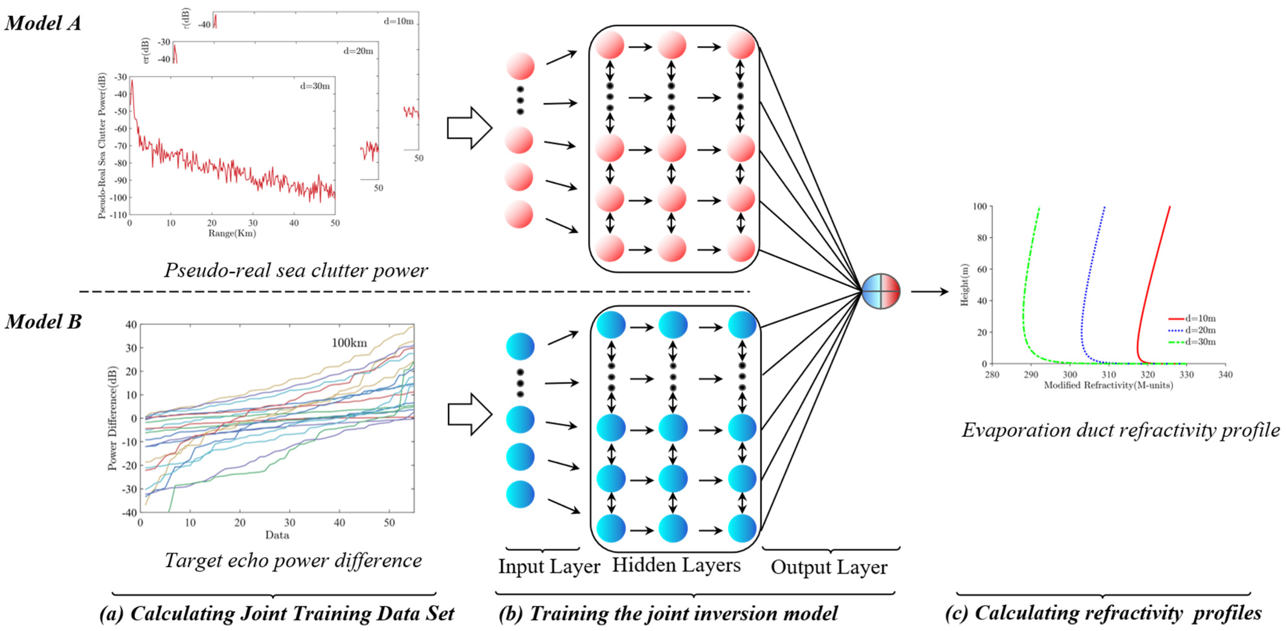
4.3. DNN-Based Joint Inversion Model Framework

Based on the above analysis, this study enhances precision of EDH inversion by introducing maritime target signals, and proposes a new model for joint inversion using radar sea clutter and over-the-horizon target signal based on DNN.

The two-stream network was proposed in 2014 by Simonyan et al. [40]. It was first applied in the field of video recognition and contains two convolutional neural network branches, which extract different input features from the video for behaviour recognition and finally fuse the two streams of information to obtain the final recognition result. The method makes up for the shortcomings of traditional two-dimensional networks in processing video data and achieves a high recognition precision. Once proposed, two-stream networks have been enthusiastically researched by many researchers, who have been conducting research on two-stream network and applying it to different fields [41].

In this paper we draw on the idea of a two-stream network, we establish a DNN-based two-stream joint inversion model, which inputs the pseudo-real sea clutter and the target signal calculated in the same duct environment into two sub-networks respectively, and then fuses the output of the two sub-networks with features in the fully connected layer to obtain the final output. The input data used to train the joint inversion model are the pseudo-real sea clutter data and the over-the-horizon target data, and the output is the corresponding EDH, so we can calculate the corresponding evaporation duct refractivity profiles. When training the joint inversion model, we still choose the ReLu function as the activation function, Adam as the optimization method and MSE as the loss function. The framework of the joint inversion model is shown in Figure 10.

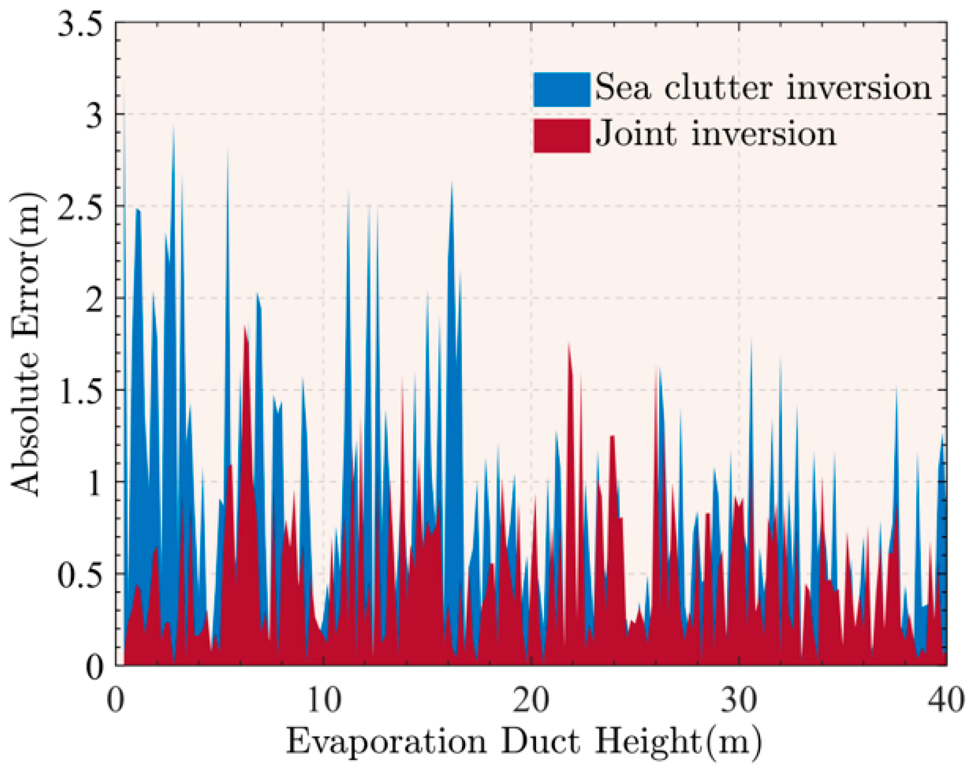
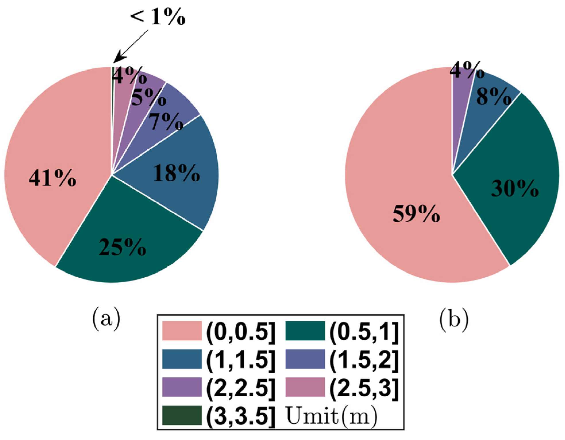
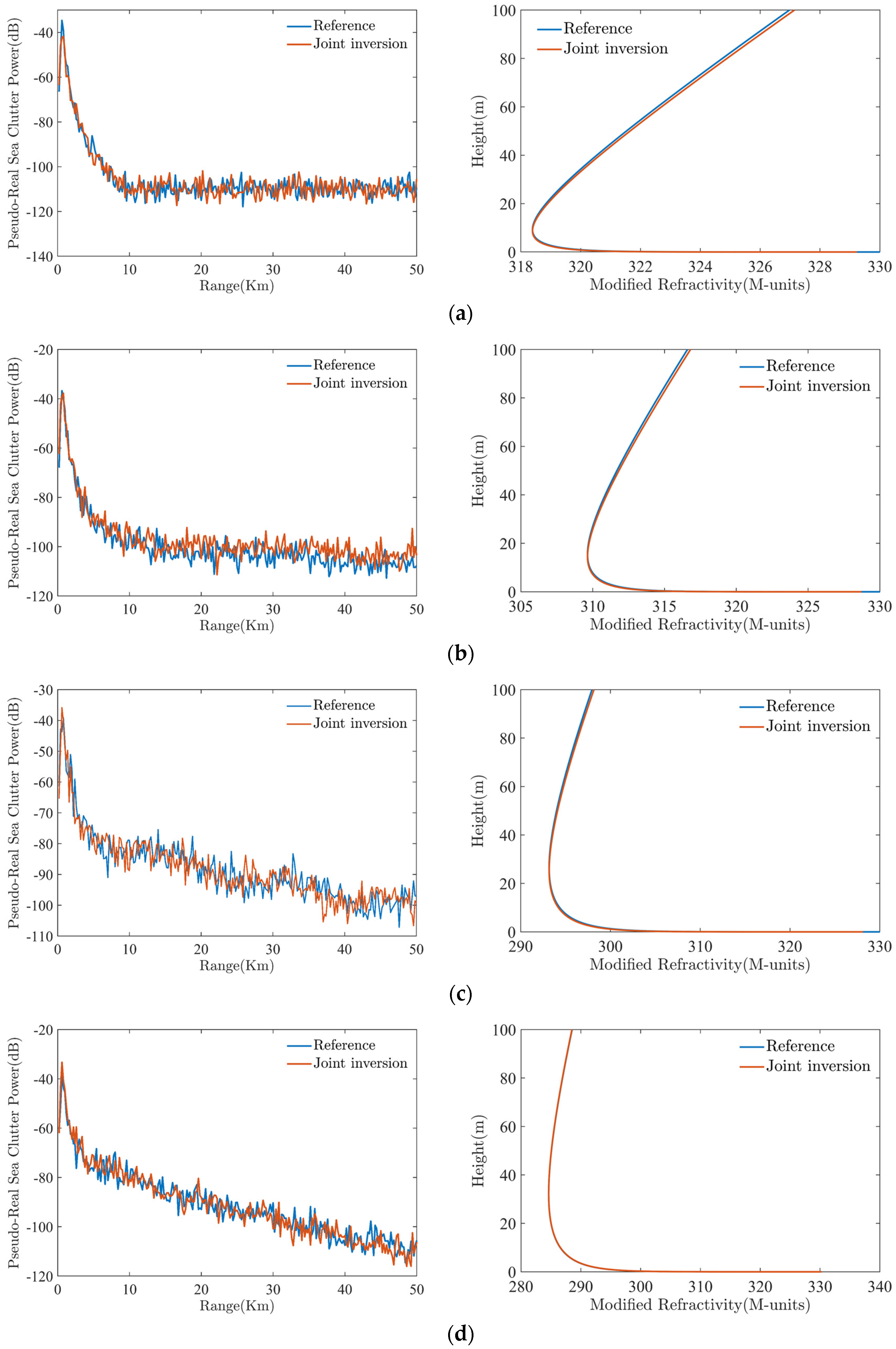
4.4. Joint Inversion and Analysis of EDH Based on Sea Clutter and Target Echo

In a certain evaporation duct environment, by adjusting the antenna height, we can obtain 55 sets of target signal power difference, based on 1000 sets of EDH, we can obtain a 1000 × 55 over-the-horizon target data matrix, and the output is a 1000 × 1 EDH matrix.

For the sub-network model A in joint inversion framework, we perform the established EDH optimal inversion model based on pseudo-real sea clutter. For the sub-network model B in joint inversion framework, similar to the conventional inversion method, we calculate a corresponding test set using the over-the-horizon target signal. The test set input is a 200 × 55 target echo signal matrix and the output is a 200 × 1 EDH matrix. After a certain number of computer experiments and comparative analysis, an optimal set of parameters (epoch: 1000, batch size: 16, hidden layer: 4) is chosen to train the EDH inversion model based on the target signal, and we finally obtain the optimal sub-network model B. The optimal joint inversion model can be obtained by combining model A and B.

The joint test set is input into the established optimal joint inversion model that calculates the absolute error at each reference height in the test set and compares it with the conventional inversion method. The experimental results are shown in Figure 11. The absolute error of the joint inversion method is significantly lower than that of the conventional method in the range of EDH from 0 to 16.7 m, which indicates that the introduction of the target signal plays a greater role in enhancing the inversion precision of the low-altitude evaporation duct. When the EDH is higher than 16.7 m, there is a part of the inversion error that is slightly higher than that of the conventional inversion method. However, on the whole, the joint inversion model has less extreme values of the difference compared with the conventional inversion method, indicating that the inversion ability of the joint model is better than that of the conventional method.

Moreover, we calculate the proportion of absolute errors in different intervals for the test sets of the two inversion methods, and the results are shown in Figure 12. The calculated results show that the EDH inversion errors of the joint inversion method and the conventional method account for 59% and 41% in the range of 0 to 0.5 m, and 30% and 25% in the range of 0.5 to 1 m, respectively. Most of the errors of the joint inversion method are distributed in the range of 0 to 1 m, accounting for a total of 89%, while the conventional method accounts for a total of 66% in the error range of 0 to 1 m, showing that the overall performance of the joint inversion method is significantly higher than that of the conventional inversion method.

To quantitatively evaluate the inversion performance of the two inversion methods, we use two types of indicators, RMSE and mean absolute error (MAE) to calculate the inversion errors of the two inversion methods. The smaller the value of the two types of indicators, the smaller the error of the inversion, the higher the precision of the inversion of the method. MAE is calculated as follows:

$$\mathrm{MAE}=\frac{{\displaystyle {\sum }_{i=1}^n\left|{\widehat{d}}_i-d_i\right|}}{n}$$

(16)

Error results based on RMSE and MAE indicators are shown in the

Table 2. Errors of Sea clutter inversion and joint inversion.

Indicator	EDH (m)	Error (m)
		Sea Clutter Inversion	Joint Inversion
RMSE	(0,16.7]	1.434	0.657
	(16.7,40)	0.741	0.621
	(0,40)	1.081	0.636
MAE	(0,16.7]	1.158	0.505
	(16.7,40)	0.587	0.481
	(0,40)	0.822	0.491

. We calculate two inversion evaluation indicators for the two inversion methods in the range of 0 to 16.7 m, 16.7 to 40 m, and 0 to 40 m for EDH, respectively. From the mean errors of EDH in the range of 0 to 40 m, the RMSE and MAE indicators of the joint inversion model are 0.636 and 0.491, respectively, which are smaller than those of the conventional inversion method, and are reduced by 41.2% and 40.3%, respectively, compared with the conventional method. It shows that the introduction of the maritime target signal has a considerable contribution to improve the inversion precision of EDH. And the two indicators of the joint inversion method are reduced by 54.2% and 56.4% compared with the conventional method in the EDH range from 0 to 16.7 m. It shows that the target echoes are more sensitive to the low-altitude evaporation duct, and effectively improves the limitation of low precision of low-altitude evaporation duct inversion that exists in the conventional method. When the EDH is more than 16.7 m, the two indicators calculated by the joint inversion method are reduced by 16.2% and 18.1%, respectively, compared with the conventional method. Although the inversion error is not reduced substantially, it is still effective for enhancing the inversion precision.

After establishing the joint inversion model with high precision, we use LHS to reselect 8.70 m, 14.56 m, 25.33 m and 32.36 m, as the reference EDH in the range of 0–40 m, and calculate the corresponding pseudo-real sea clutter power and target echo power. We input the above validation data into the established optimal joint inversion model to obtain the EDH inversion results, so as to calculate the corresponding evaporation duct refractivity profiles, as shown in Figure 13. In Figure 13, the joint inverted evaporation duct refractivity profiles are close to the reference values, and high inversion precision is obtained. The results obtained by the joint inversion method are shown in

Table 3. Results of joint inversion method.

Reference EDH	Result	Error (m)
d = 8.70	9.26	0.56
d = 14.56	15.45	0.89
d = 25.33	26.58	1.25
d = 32.36	32.19	0.17

. Although the inversion results have some errors with the reference values, they are within acceptable ranges. The inverse error is minimized to 0.17 m when the EDH is 32.36 m. Additionally, with the addition of noise, the small error between the joint inverted profile and the reference profile is maintained, showing that using DNN to perform inversion yields good anti-noise performance.

5. Conclusions

In this study, a new method is proposed for the first time to jointly invert the refractivity profile parameter of evaporation duct using sea clutter and over-the-horizon target signal. To address the limitations of using conventional method to invert the atmospheric refractivity profile parameter of low-altitude evaporation duct. Two experiments are performed to compare the inversion performance and test the noise immunity to explore the comprehensive performance of the joint inversion model. To train the established new model, firstly, we sample multiple sets of EDH samples in the height range from 0 to 40 m and calculate the corresponding pseudo-real sea clutter power, and propose a method to use the maritime over-the-horizon signal in practical situations according to the RCS features of the target. Pseudo-real sea clutter power and difference of the target echo are jointly formed into a joint data set, which is applied to the inversion problem of EDH. The experimental results show that the RMSE and MAE of the joint inversion model are smaller than those of the conventional method in the EDH range from 0 to 16.7 m, and they are 54.2% and 56.4% lower than those of the conventional method, respectively. It indicates that the introduction of the target echo power effectively improves the limitations of low precision of the inversion of low-altitude EDH existing in the conventional method. The anti-noise performance is tested to show that the inverse evaporation duct refractivity profile matches well with the sample reference profile, and the inverse error is minimized to 0.17 m when the EDH is 32.36 m. The joint inversion model has excellent comprehensive performance and successfully breaks through the limitations of conventional inversion methods, and its outstanding advantages provide an effective and reliable technical means for precise inversion of EDH.

References

1. Yan, X.D.; Yang, K.D.; Ma, Y.L. Calculation Method for Evaporation Duct Profiles Based on Artificial Neural Network. IEEE Antennas Wirel. Propag. Lett. 2018, 17, 2274–2278. [Google Scholar] [CrossRef]
2. Barrios, A.E. Parabolic equation modeling in horizontally inhomogeneous environments. IEEE Trans. Antennas Propag. 1992, 40, 791–797. [Google Scholar] [CrossRef] [Green Version]
3. Dang, M.X.; Wu, J.J.; Cui, S.C.; Guo, X.; Cao, Y.H.; Wei, H.L.; Wu, Z.S. Multiscale Decomposition Prediction of Propagation Loss in Oceanic Tropospheric Ducts. Remote Sens. 2021, 13, 1173. [Google Scholar] [CrossRef]
4. Musson Genon, L.; Gauthier, S.; Bruth, E. A simple method to determine evaporation duct height in the sea surface boundary layer. Radio Sci. 1992, 27, 635–644. [Google Scholar] [CrossRef]
5. Anderson, K.D. Radar measurements at 16.5 GHz in the oceanic evaporation duct. IEEE Trans. Antennas Propag. 1989, 37, 100–106. [Google Scholar] [CrossRef] [Green Version]
6. Lionis, A.; Peppas, K.; Nistazakis, H.E.; Tsigopoulos, A.D.; Cohn, K. Experimental Performance Analysis of an Optical Communication Channel over Maritime Environment. Electronics 2020, 9, 1109. [Google Scholar] [CrossRef]
7. Han, J.; Wu, J.J.; Zhu, Q.L.; Wang, H.G.; Zhou, Y.F.; Jiang, M.B.; Zhang, S.B.; Wang, B. Evaporation Duct Height Nowcasting in China’s Yellow Sea Based on Deep Learning. Remote Sens. 2021, 13, 1577. [Google Scholar] [CrossRef]
8. Xie, F.; Dong, M.Z.; Wang, X.T.; Yan, J. Infrared Small-Target Detection Using Multiscale Local Average Gray Difference Measure. Electronics 2022, 11, 1547. [Google Scholar] [CrossRef]
9. Fountoulakis, V.; Earls, C. Inverting for Maritime Environments Using Proper Orthogonal Bases From Sparsely Sampled Electromagnetic Propagation Data. IEEE Trans. Geosci. Remote Sens. 2016, 54, 7166–7176. [Google Scholar] [CrossRef]
10. Rogers, L.T.; Hattan, C.P.; Stapleton, J.K. Estimating evaporation duct heights from radar sea echo. Radio Sci. 2000, 35, 955–966. [Google Scholar] [CrossRef] [Green Version]
11. Vasudevan, S.; Krolik, J.L. Refractivity estimation from radar clutter by sequential importance sampling with a Markov model for microwave propagation. In Proceedings of the 2001 IEEE International Conference on Acoustics, Speech, and Signal Processing, Salt Lake City, UT, USA, 7–11 May 2001. [Google Scholar]
12. Gerstoft, P.; Rogers, L.T.; Krolik, J.L.; Hodgkiss, W.S. Inversion for refractivity parameters from radar sea clutter. Radio Sci. 2003, 38, 11–18. [Google Scholar] [CrossRef]
13. Barrios, A.E. Estimation of surface-based duct parameters from surface clutter using a ray trace approach. Radio Sci. 2004, 39, 1–9. [Google Scholar] [CrossRef]
14. Yardim, C.; Gerstoft, P.; Hodgkiss, W.S. Estimation of radio refractivity from Radar clutter using Bayesian Monte Carlo analysis. IEEE Trans. Antennas Propag. 2006, 54, 1318–1327. [Google Scholar] [CrossRef]
15. Yardim, C.; Gerstoft, P.; Hodgkiss, W.S. Statistical maritime radar duct estimation using hybrid genetic algorithm–Markov chain Monte Carlo method. Radio Sci. 2007, 42, RS3014. [Google Scholar] [CrossRef] [Green Version]
16. Wan, R.Z.; Tian, C.D.; Zhang, W.; Deng, W.D.; Yang, F. A Multivariate Temporal Convolutional Attention Network for Time-Series Forecasting. Electronics 2022, 11, 1516. [Google Scholar] [CrossRef]
17. Guo, X.W.; Wu, J.J.; Zhang, J.P.; Han, J. Deep learning for solving inversion problem of atmospheric refractivity estimation. Sust. Cities Soc. 2018, 43, 524–531. [Google Scholar] [CrossRef]
18. Li, G.; Cai, H.Z.; Li, C.F. Alternating Joint Inversion of Controlled-Source Electromagnetic and Seismic Data Using the Joint Total Variation Constraint. IEEE Trans. Geosci. Remote Sens. 2019, 57, 5914–5922. [Google Scholar] [CrossRef]
19. Alekseev, A.S. Quantitative statement and general properties of solutions of cooperative inverse problems (integral geophysics). SEG Abstr. 1991, 61, 1021–1022. [Google Scholar]
20. Cai, H.Z.; Zhdanov, M. Joint Inversion of Gravity and Magnetotelluric Data for the Depth-to-Basement Estimation. IEEE Trans. Geosci. Remote Sens. 2017, 14, 1228–1232. [Google Scholar] [CrossRef]
21. Haack, T.; Wang, C.; Garrett, S.; Glazer, A.; Mailhot, J.; Marshall, R. Mesoscale Modeling of Boundary Layer Refractivity and Atmospheric Ducting. J. Appl. Meteorol. Clim. 2010, 49, 2437–2457. [Google Scholar] [CrossRef]
22. Douvenot, R.; Fabbro, V.; Gerstoft, P.; Bourlier, C.; Saillard, J. Real time refractivity from clutter using a best fit approach improved with physical information. Radio Sci. 2010, 45, 1–13. [Google Scholar] [CrossRef] [Green Version]
23. Zhang, J.P.; Wu, Z.S.; Hu, R.X. Combined Estimation of Low-Altitude Radio Refractivity Based on Sea Clutters from Multiple Shipboard Radars. J. Electromagn. Waves Appl. 2011, 25, 1201–1212. [Google Scholar] [CrossRef]
24. Yang, C. Estimation of the Atmospheric Duct from Radar Sea Clutter Using Artificial Bee Colony Optimization Algorithm. Prog. Electromagn. Res. 2013, 135, 183–199. [Google Scholar] [CrossRef] [Green Version]
25. Wang, M.N.; Wang, Z.; Cheng, Z.; Chen, J. Target detection for a kind of troposcatter over-the-horizon passive radar based on channel fading information. IET Radar Sonar Nav. 2018, 12, 407–416. [Google Scholar] [CrossRef]
26. Dong, X.; Sun, F.; Zhu, Q.L.; Lin, L.K.; Zhao, Z.W.; Zhou, C. Tropospheric Refractivity Profile Estimation by GNSS Measurement at China Big-Triangle Points. Atmosphere 2021, 12, 1468. [Google Scholar] [CrossRef]
27. Zhang, J.P.; Wu, Z.S.; Zhu, Q.L.; Wang, B. A Four-Parameter M-Profile Model for the Evaporation Duct Estimation from Radar Clutter. Prog. Electromagn. Res. 2011, 114, 353–368. [Google Scholar] [CrossRef] [Green Version]
28. Compaleo, J.; Yardim, C.; Xu, L.Y. Refractivity-From-Clutter Capable, Software-Defined, Coherent-on-Receive Marine Radar. Radio Sci. 2021, 56, 1–19. [Google Scholar] [CrossRef]
29. Zhou, S.; Gao, H.T.; Ren, F.Y. Pole Feature Extraction of HF Radar Targets for the Large Complex Ship Based on SPSO and ARMA Model Algorithm. Electronics 2022, 11, 1644. [Google Scholar] [CrossRef]
30. Barcaroli, E.; Lupidi, A.; Facheris, L.; Cuccoli, F.; Chen, H.N.; Chandra, C.V. A Validation Procedure for a Polarimetric Weather Radar Signal Simulator. IEEE Trans. Geosci. Remote Sens. 2019, 57, 609–622. [Google Scholar] [CrossRef]
31. Broschat, S.L. The small slope approximation reflection coefficient for scattering from a “Pierson-Moskowitz” sea surface. IEEE Trans. Geosci. Remote Sens. 1993, 31, 1112–1114. [Google Scholar] [CrossRef] [Green Version]
32. Zhang, H.W.; Zhang, Y.S.; Li, Z.W.; Liu, B.Y.; Yin, B.; Wu, S.H. Small Angle Scattering Intensity Measurement by an Improved Ocean Scheimpflug Lidar System. Remote Sens. 2021, 13, 2390. [Google Scholar] [CrossRef]
33. Posner, F.L. Spiky sea clutter at high range resolutions and very low grazing angles. IEEE Trans. Aerosp. Electron. Syst. 2002, 38, 58–73. [Google Scholar] [CrossRef]
34. Ma, L.W.; Wu, J.J.; Zhang, J.P.; Wu, Z.S.; Jeon, G.; Tan, M.Z.; Zhang, Y.S. Sea Clutter Amplitude Prediction Using a Long Short-Term Memory Neural Network. Remote Sens. 2019, 11, 2826. [Google Scholar] [CrossRef] [Green Version]
35. Weiner, M.M. Noise factor and antenna gains in the signal/noise equation for over-the-horizon radar. IEEE Trans. Aerosp. Electron. Syst. 1991, 27, 886–890. [Google Scholar] [CrossRef]
36. Chen, H.W.; Li, X.; Jiang, W.D.; Zhuang, Z.W. MIMO Radar Sensitivity Analysis of Antenna Position for Direction Finding. IEEE Trans. Signal Process. 2012, 60, 5201–5216. [Google Scholar] [CrossRef]
37. Kim, N.; Shin, D.; Choi, W.; Kim, G.; Park, J. Exploiting Retraining-Based Mixed-Precision Quantization for Low-Cost DNN Accelerator Design. IEEE Trans. Neural Netw. Learn. Syst. 2021, 32, 2925–2938. [Google Scholar] [CrossRef]
38. Qiao, C.; Li, D.; Guo, Y.T.; Liu, C.; Jiang, T.; Dai, Q.H.; Li, D. Evaluation and development of deep neural networks for image super-resolution in optical microscopy. Nat. Methods 2021, 18, 194–202. [Google Scholar] [CrossRef]
39. Ren, F.Y.; Gao, H.T.; Yang, L.J. Distributed Multistatic Sky-Wave Over-The-Horizon Radar Based on the Doppler Frequency for Marine Target Positioning. Electronics 2021, 10, 1472. [Google Scholar] [CrossRef]
40. Piwowarski, P.; Kasprzak, W. Evaluation of Multi-Stream Fusion for Multi-View Image Set Comparison. Appl. Sci. 2021, 11, 5863. [Google Scholar] [CrossRef]
41. Yan, Q.S.; Gong, D.; Zhang, Y.N. Two-Stream Convolutional Networks for Blind Image Quality Assessment. IEEE Trans. Image Process. 2019, 28, 2200–2211. [Google Scholar] [CrossRef]
Figure 1. Effects of tropospheric duct on radar performance.
Electronics 11 02157 g001
Figure 2. Modified refractivity profiles for different EDHs.
Electronics 11 02157 g002
Figure 3. Sea clutter power for different EDHs: (a) EDHs range from 2 m to 20 m; (b) EDHs range from 22 m to 40 m.
Electronics 11 02157 g003
Figure 4. Simulation clutter power and pseudo−real sea clutter for different EDHs: (a) EDH = 10 m; (b) EDH = 20 m; (c) EDH = 30 m.
Electronics 11 02157 g004
Figure 5. DNN−based EDH inversion model.
Electronics 11 02157 g005
Figure 6. Absolute errors of sea clutter inversion.
Electronics 11 02157 g006
Figure 7. Target echoes at different antenna heights.
Electronics 11 02157 g007
Figure 8. Target echo data at different locations on the sea surface for different EDHs. Sea surface target position at: (a) 10 km; (b) 20 km; (c) 30 km; (d) 40 km; (e) 70 km; (f) 100 km.
Electronics 11 02157 g008
Figure 9. MAD values at different locations on sea surface.
Electronics 11 02157 g009
Figure 10. DNN−based joint inversion model framework.
Electronics 11 02157 g010
Figure 11. Absolute errors of the joint inversion method and the sea clutter inversion method.
Electronics 11 02157 g011
Figure 12. The proportion of errors in different intervals for the two inversion methods. Errors of (a) sea clutter inversion; (b) joint inversion.
Electronics 11 02157 g012
Figure 13. Comparison of refractivity profile and pseudo−real sea clutter power estimations results to reference EDHs: (a) d = 8.70 m; (b) d = 14.56 m; (c) d = 25.33 m; (d) d = 32.36 m.
Electronics 11 02157 g013