The 3D Position Estimation and Tracking of a Surface Vehicle Using a Mono-Camera and Machine Learning

Abstract

The ability to obtain the 3D position of target vehicles is essential to managing and coordinating a multi-robot operation. We investigate an ML-backed object localization and tracking system to estimate the target’s 3D position based on a mono-camera input. The passive vision-only technique provides a robust field awareness in challenging conditions such as GPS-denied or radio-silent environments. Our processing pipeline utilizes a YOLOv5 neural network as the back-end detection module and a temporal filtering technique to improve detection and tracking accuracy. The filtering process effectively removes false positive labels to improve tracking accuracy. We propose a piecewise projection model to predict the target 3D position from the estimated 2D bounding box. Our projection model utilizes the co-plane property of ground vehicles to calculate 2D–3D mapping. Experimental results show that the piecewise model is more accurate than existing methods when the training dataset is not evenly distributed in the sampling space. Our piecewise model outperforms the singular RANSAC-based and the 6DPose methods by 28% in location errors. A less than 10-m error is observed for most near-to-mid-range cases.

1. Introduction

Vision-based object detection and tracking have played significant roles in surveillance, unoccupied vehicle (UxV) control, and motion planning of autonomous robots. As the number of unoccupied systems and robots increases in application fields, multiple levels of situation awareness are needed to provide safety assurance for planning and coordinating robot movement. For example, in a busy warehouse where both human operators and robot movers operate in close range, the positions of the moving objects must be closely monitored for apparent reasons. Based on realtime position information, a centralized or distributed scheduler such as Rapidly-exploring Random Trees (RRTs) [1] can be used to generate a safe motion plan for all robots.

To obtain the position of relevant objects, a commonly used method is self-reporting: each participating robot will constantly transmit its Global Position System (GPS) coordinates or local position to the central scheduler. The accuracy of the local position can be in the range of center-meters in some cases when ultra wideband ranging sensors are used, thus allowing very high scheduling efficiency. However, this self-reporting method is not suitable if the target objects are not able or unwilling to report their position, which is the motivation of our work.

An alternative is a computer vision-based method that estimates an interesting target’s position from the camera data. The technique has a few unique benefits: it is passive and does not rely on self-position-reporting, and it is a robust technology that performs well in many harsh environments (such as GPS-denied scenarios). Computer vision has been very successful in object recognition and tracking. Even before discovering deep learning object detection CNNs such as the YOLO (You Only Look Once) network, conventional object tracking algorithms were capable of finding the best matching bounding box in video frames that contain the same target object.

Research Gap

The major research gap is the lack of an accurate method to directly estimate the 3D position of an object from mono-camera input. In computer vision, the problem is partially tackled by using a calibrated stereo camera and a regression technique such as RANSAC [2] to optimize the camera model parameters. The algorithm developed for stereo settings is not applicable to a mono-camera. Recently, deep neural networks have been trained [3,4] to directly predict the target 3D or 6D pose. However, these methods perform poorly when the object footprint is small, e.g., at a far distance. To the best of our knowledge, there is little reported success in estimating the object’s 3D position based on vision data.

We investigate a novel vision-based method to estimate the 3D location of an object from 2D camera observations in a pseudo-planner setting. Our particular application is to estimate the positions of small surface vehicles in a waterway traffic hub such as a seaport. The goal is to detect a target boat from a live video feed and determine its absolute or relative coordinates. This project was created in response to the Navy challenge “AI Track at Sea” in 2020. The challenge provides a training dataset consisting of video clips of a moving boat and a subset of the corresponding 3D positions. The objective is to develop a predictive model that can predict the 3D location of the target from a similar video/imaging source. Such a system would provide at least a redundant means for traffic control in a busy port (Figure 1) or path planning of autonomous boats in the area.

Estimating an object’s 3D pose from a 2D view has long been recognized as an ill-posed problem in computer vision. A single 2D observation of an object admits infinite 3D candidate solutions with an ambiguous scale. For a true 3D solution, one potential method is to train an end-to-end 6D pose estimation using multiple 2D images, with which we have had some success in short-range scenarios. The approach we will discuss in this work does not seek 6D estimation due to the diminished features of the faraway objects. Instead, we explore a technique that combines 2D object tracking and piecewise modeling of the camera projection to estimate the near co-plane objects.

Our main contributions can be summarized as follows:

(1)

We evaluated a novel processing pipeline to extract the 3D position of the target from a mono-camera video source;

(2)

We investigated a novel temporal filter based on the confidence value and spatial locality of the object bounding box to improve object tracking. The filtering algorithm allows us to fill in the holes in the predicted boat location and regenerate missing prediction in some cases;

(3)

We proposed a search method to optimize a piecewise camera model to predict an object’s 3D positions. Our search method is adaptive as it considers the training dataset’s distribution when determining the boundary of the piecewise submodel.

The entire processing pipeline is evaluated on an NVIDIA Jetson TX2 embedded computer. Our overall implementation achieves real-time and satisfactory performance in terms of both accuracy and speed (video demo accessed on 4 February 2021 https://youtu.be/cZVd9LtjnsY_). Our piecewise model outperforms the singular RANSAC-based method by 28% in location errors. A less than 10 m error is observed for most near-to-mid-range cases.

In the rest of the paper, Section 3 discusses the overall system architecture and the neural network training for target detection. Section 4 discusses the filtering algorithm to improve the detection results using the inherent temporal correlation within consecutive video frames. Section 5 discusses the piecewise camera model to estimate the 3D position from the corrected 2D position. Section 6 presents the experimental results.

2. Related Works

Determining an object’s 3D position from a 2D image is an ill-posed computer vision problem since the depth information is lost during the perspective projection. The solution to the problem nevertheless is enormously useful for path planning [1]. The most relevant work in object detection focuses on 2D object detection and tracking. In the 3D domain, many published works focus on reconstructing the object’s 3D model [5,6], but there is little emphasis on determining the object’s 3D position. Typical RGB-D cameras have a very short effective range (<10 m), rendering them useless in most practical applications. The depth from stereo has been studied for a long time [7,8]; however, most works also focus on object scenes at a short distance. Furthermore, methods developed for stereo cameras are not suited for mono-camera input.

In similar work [9], the authors proposed a deep learning network to estimate the 6D pose of objects. However, our experiments show that the method has a high z-axis (distance) error for objects that are more than a few meters away. A modified implementation of their method was evaluated on our dataset for comparison, showing an inferior performance to ours.

Considering the robotic control stack more broadly, the computational result of our work is consumed by a high-level path planning entity for single or multi-robot navigation control. Multi-robot path planning [10,11,12] and optimization have been gaining more attention recently. In most published works, two-phase planning is used where the first phase constructs roadmaps via conventional sampling-based motion planning (SBMP) or lattice grids, and the second phase often uses multi-agent pathfinding (MAPF) algorithms [12]. Obviously, all of the later-mentioned planning algorithms require accurate knowledge of both static and dynamic obstacles, which is the focus of our work.

Object detection and tracking: Traditional object detection methods combine feature detection with a machine learning classification algorithm such as KNN (K Nearest Neighbors) or SVM (Support Vector Machines). Notable feature detection algorithms include SIFT [13] and SURF (Speeded Up Robust Features). These feature descriptors are scale-invariant [14] representations of the image using a series of mathematical approximations. These features are also applicable to detect and classify objects in various applications [3,9]. The effectiveness and robustness of such a method in real-world applications are affected by multiple factors such as the movement speed of surrounding objects, lighting conditions, and scene occlusions. Building a system with both high accuracy and real-time performance is particularly challenging with an embedded system due to the limited computing resources. Object tracking techniques with RGB-T cameras are discussed in [15,16,17]. The authors of [18] discussed a method to track an object in motion video by exploiting the correlation of poses in the video. Our paper uses a similar idea to improve the the detected object positions.

Deep learning object detection: Feature extraction algorithms such as SIFT and SURF require a lot of computing power. End-to-end trainable deep neural networks such as region-based CNNs (R-CNNs) [19] have been introduced as faster object detection algorithms. Instead of feeding the region proposals to the CNN, the CNN’s input image is fed to generate a convolutional feature map. Faster R-CNN has been proposed to solve the bottleneck by the region proposal algorithm. It consists of a CNN called the Region Proposal Network (RPN) as a region proposal algorithm and the Fast R-CNN as a detector. You Only Look Once (YOLO) [15] is one of the most widely used object detection methods. YOLO can process realtime video with a minimal delay while maintaining excellent accuracy. In our work, we use the YOLOv5 version, which has several subversions depending on the available GPU memory. The Single Shot MultiBox Detector (SSD) was a worthy alternative. The SSD uses a single forward propagation of the network in the same way as YOLO and passes the input image through a series of convolutional layers to generate candidate bounding boxes at various scales. In [17], Zhang et al., used a Modality-aware Filter Generation Network (named MFGNet) for RGB-T tracking. The MFGNet network adaptively adjusts the convolutional filters when both thermal and RGB data are present. It is also noteworthy that simple image preprocessing techniques such as dehazing did not substantially improve the vision model’s performance [20,21]. Hence, our method did not use such a technique to sharpen the image quality of faraway boats.

3. Detection Network Training

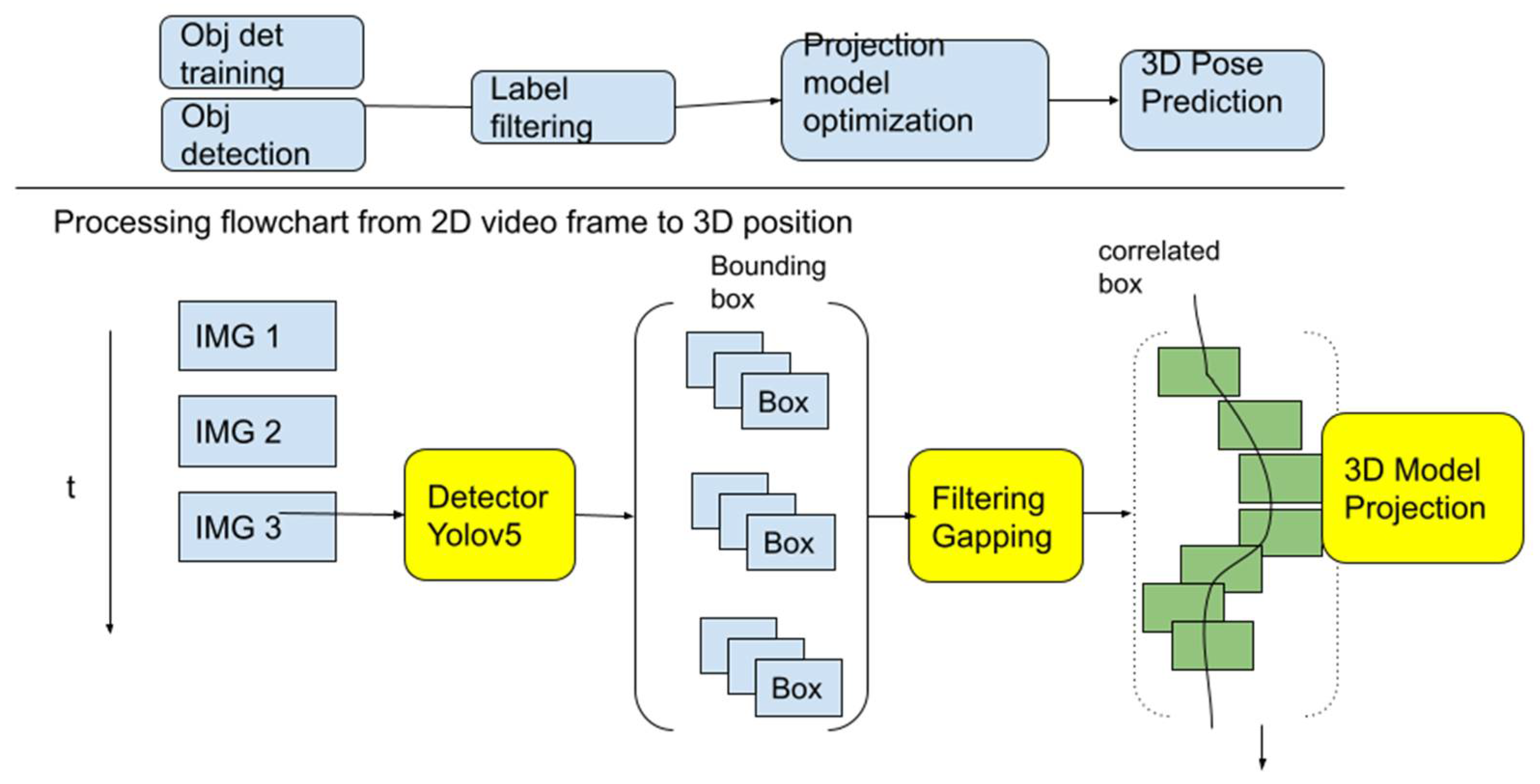
Our proposed processing pipeline is illustrated in Figure 2. It consists of three main components: (1) a YOLOv5 neural network to detect the 2D bounding box of the target boats, (2) a filter algorithm to remove false positives and to correct mis-labeled detection, and (3) a piecewise 3D projection model to generate the desired 2D–3D mapping. The YOLOv5 network is fast and adaptable for transfer learning new datasets. For each input video frame, the YOLOv5 network will detect potential targets and generate 2D bounding boxes along with their classifications. A well-trained network can accurately estimate the 2D bounding box within a few pixels. We will discuss the details of the network training in the rest of the section.

However, similar to many other deep learning object detection systems, the detection probability and the accuracy of the YOLOv5 detector degrade quickly for small and faraway objects. This performance degradation is inherent and cannot be completely eliminated at the detector level. This is mitigated by a temporal filter algorithm that will be discussed in Section 4. The output of the filter is a corrected version of the 2D bounding boxes, which represent a continuous trajectory of the target object. At the final step, the corrected 2D boxes are back-projected to a 3D position (see Section 5).

3.1. Dataset and Preprocessing

The raw training data consisted of two parts: (1) 12 video clips recorded by a webcam at an observation deck and (2) a corresponding GPS log measured by a COTS GPS sensor onboard the target boat. The two recordings were only synchronized at the start time and each used its local clock during the data collection period.

A practical issue in transfer training of deep CNNs for a real-world dataset is the potential noise introduced during the annotation process. In our case, the detector network was trained with manually labeled video frames. Furthermore, a good portion of the ground truth 3D position was purposely removed with the hope of a more robust solution for poor data quality.

For each video frame extracted from the video, we created a target boat label in YOLOv5 format manually. The image frames were aligned with the ground truth location data from the GPS logger. However, the GPS logger data points were very sparse and only came in about every 5 s, much slower than the 30 f/s video frame. Therefore, there were many video frames without a GPS tag. Some data points were considered not usable if the target boat was too small to be detected by human eyes. After removal of the unusable data points, the initial training data set consisted of 851 frames.

3.2. Object Detection Training Result

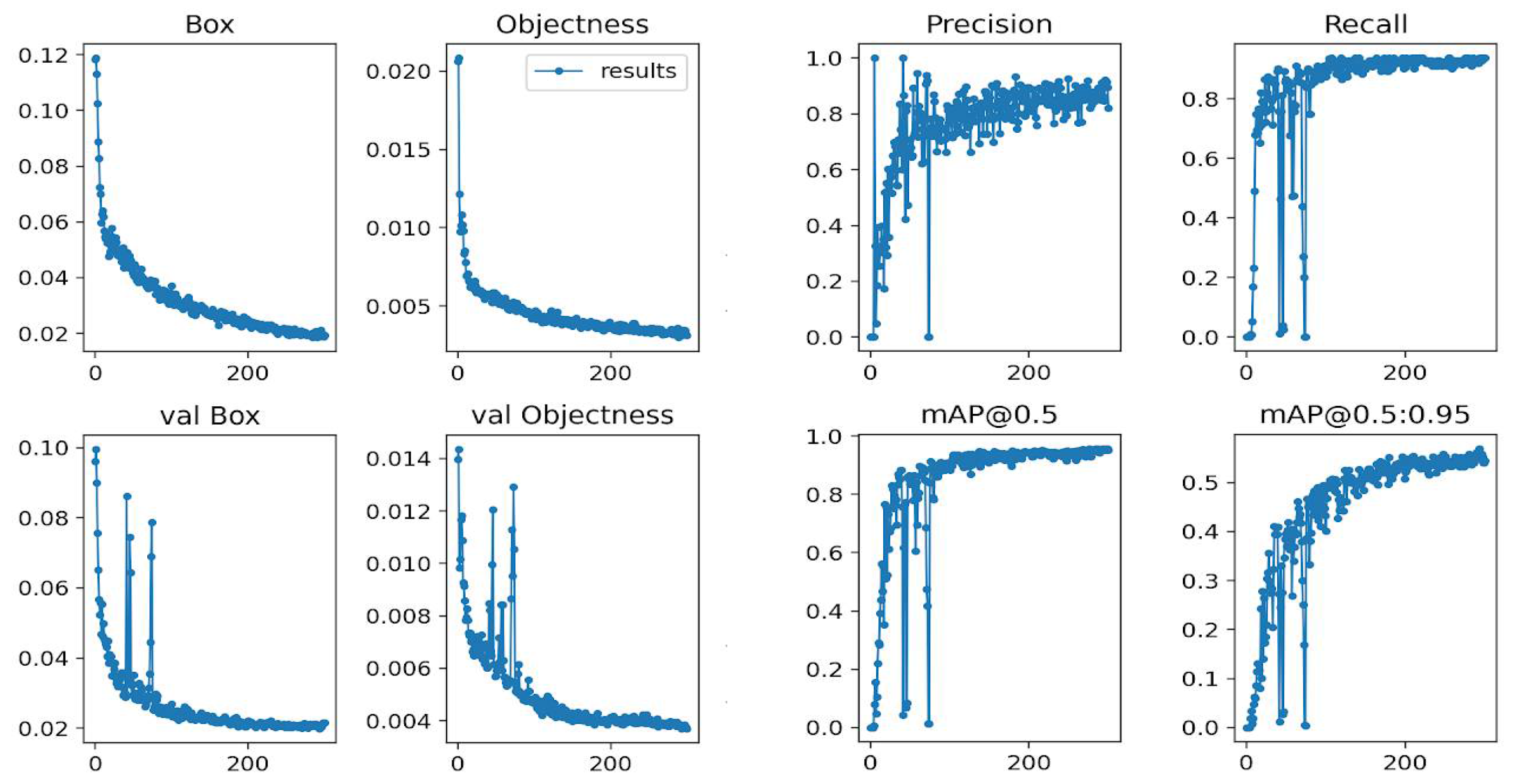
The initial training set only contained the label for the target boat. Other objects in the video scene were not used. We used the pre-trained YOLOv5 small parameter weights for the feature extraction part of the network and retrained only the last three layers. The network was trained for 300 epochs with a batch size of 8 and an initial learning rate of 0.001. The learning rate was down-adjusted at 30 and 60 epochs. In the NVIDIA TX2 module, the training time is about 5 h. The training and recall results are shown in Figure 3.

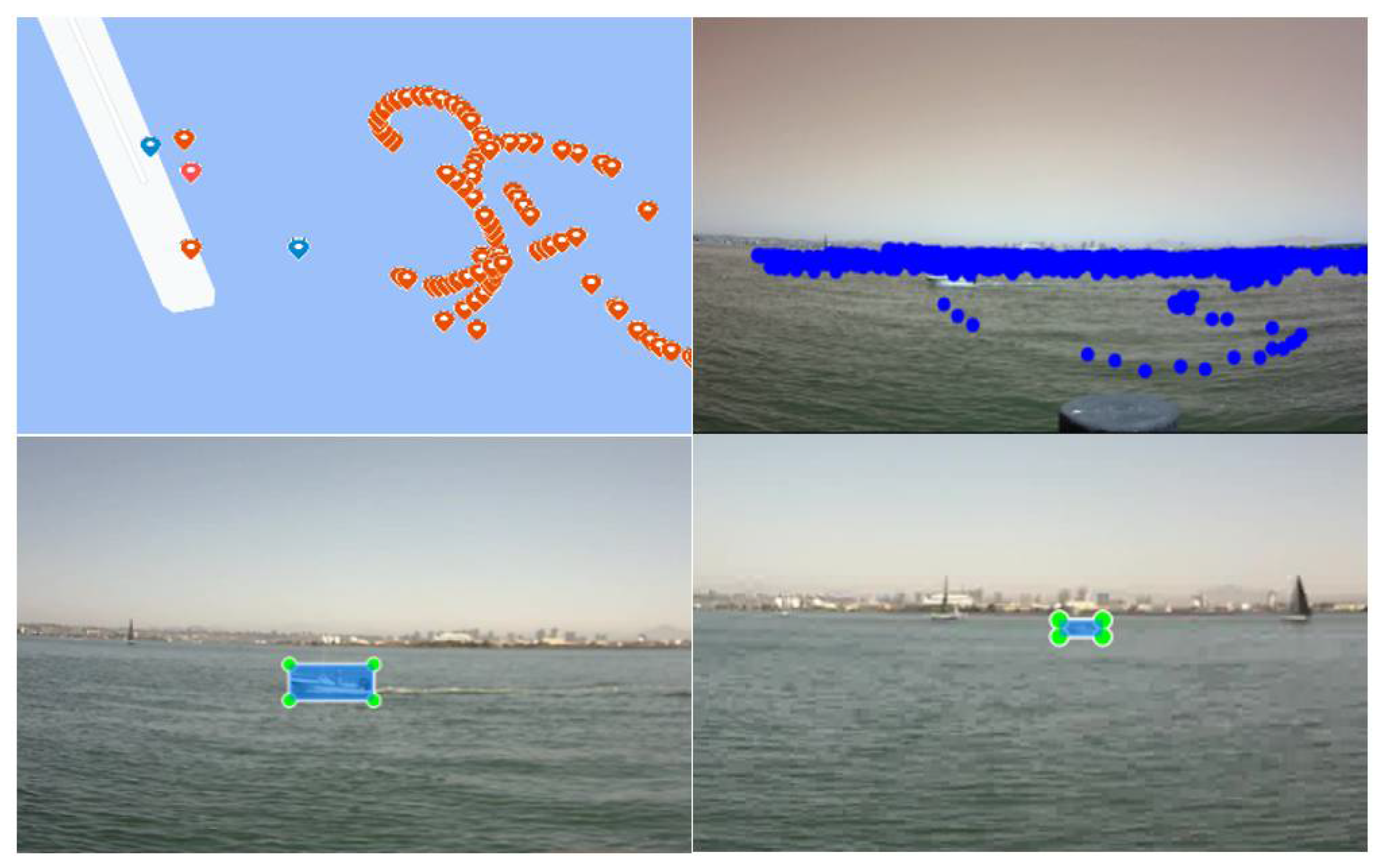
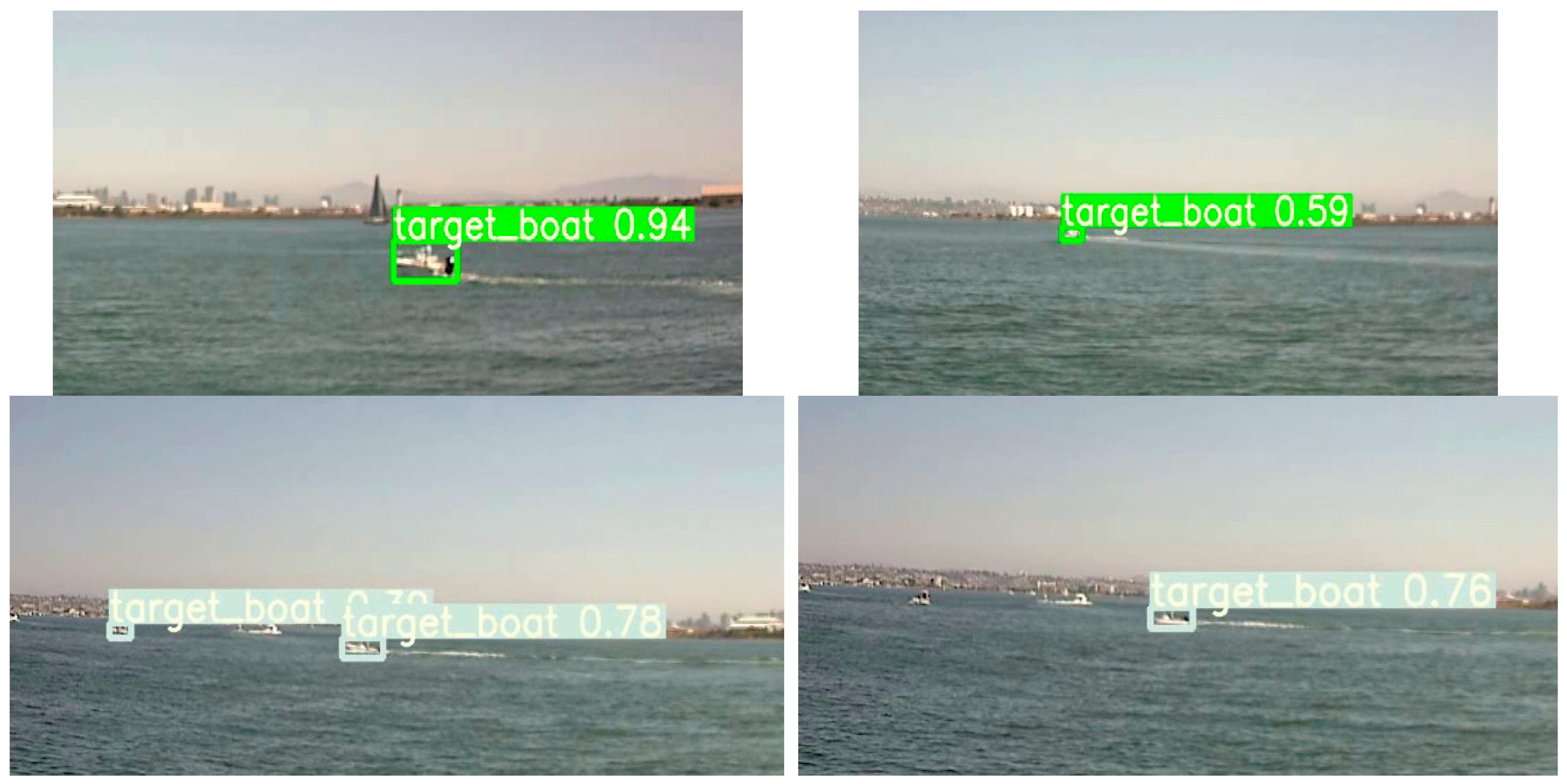
We quickly noticed that the initial trained model produced a significant number of false positives due to the lack of negative examples. The error cases included mistaking other boats as the target boat. Further, other objects such as seagulls or a different boat were detected as the target boat in some instances.

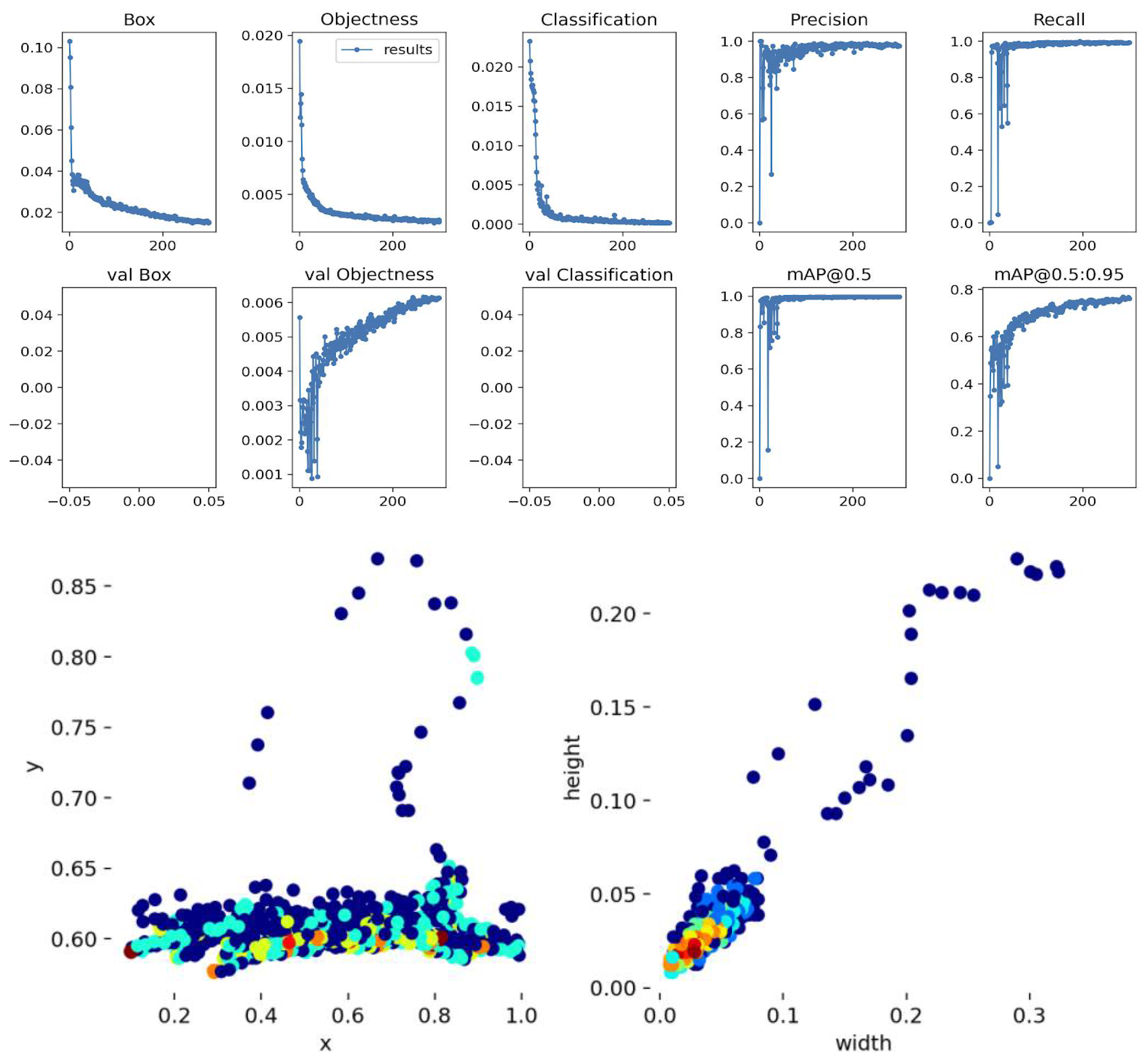
We added additional labels to the training data set to reduce the false positive detection. Three new classes were “OB1”, “OB2”, and “BIRD”. The network was retrained with the same hyperparameters, and the results are shown in Figure 4. The retrained network showed a much better false positive rate. We observed that the remaining classification errors occurred when (1) the target boat and the mistaken boat were very similar or (2) the mistaken boat was far away and had a tiny image footprint (tens of pixels). Figure 4 (bottom) shows that the low confidence (orange color) cases were concentrated on distant target objects. We believe that further improvement in target detection would be difficult without causing severe model overfitting. Hence, we decided to leave these errors to be handled at the filtering stage, where we could leverage temporal information to correct errors.

4. Temporal Filter and Missing Label Prediction

We now discuss the temporal filter design to improve the object detection result further. Here, the term filtering means that information in the past or future can be used to reject or change the label of the bounding boxes in the current frame. As mentioned earlier, there are two types of errors in the output of the boat detector. The first is that the network cannot detect the target boat too far away (i.e., too small a footprint in the image). About 20% of the images had a 2D bounding box with fewer than 10 × 20 pixels in the training dataset. These images were difficult even to a trained human eye since they barely contained enough usable features for detection and discrimination. The network also had difficulty correctly detecting the target when there was significant occlusion with other objects. This problem is evident in one of the test videos (https://youtu.be/cZVd9LtjnsY accessed on 4 February 2021), where we show the detector output without filter and tracking. Some of the missed detections were due to the low confidence values of the detection result. With our proposed tracker, the problem was partially solved as long as the YOLO detector provided a suitable bounding box. A more comprehensive treatment would require the modification of the object detector to produce a list of bounding boxes, which will be explored in our future research.

The second problem is that the network might classify other boats or objects as the target boat when the appearances are similar. The two issues boil down to the common problem in all image processing methods: similar objects are challenging to be distinguished at a far distance as their distinct features diminish. It is noteworthy that the object detection neural network often overfits if force-trained to separate such extreme cases.

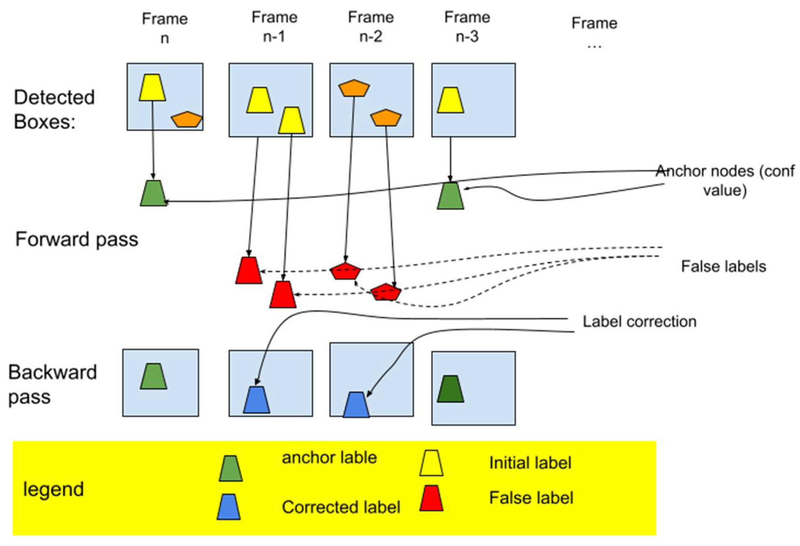
A widely used technique to improve object detection and tracking is to exploit the temporal correlation between consecutive video frames, which we refer to as temporal filtering. Our proposed filter algorithm adopts a two-pass design to examine and correct the labeling of the detected bounding boxes of the past n frames. As shown in Figure 5, we first used a forward pass to filter out all “bad” labels that had a low confidence level (we used a threshold $con{f}_l=0.3$). The pseudo-code for forward pass is given at Algorithm 1. This helped eliminate the more pronounced false-positive detections. The first pass also identified a set of anchor nodes with a high confidence level $( con{f}_h=0.7$). The forward pass resulted in some detection holes in some video frames as we relabeled the low-confidence bounding box as false-positive cases.

The second pass is a backward passing (see Algorithm 2) where the remaining false positives and false negatives were handled. During the filtering process, we calculated an adjusted likelihood for all non-anchor nodes. The adjusted-likelihood value is defined as follows:

$$pro{b}_i=dist\_box\left(n_i,a_i\right)*conf\left(a_i\right).$$

Algorithm 1: TF Forward Pass

//process box[1…n] conf[1…n], label[1…n]

For each conf[i]:

If conf[i] < conf_l

Label[i]= −1 // change the label to uncertain

If conf[i] > conf_h

Label[i]= ANCHOR

Insert box[i] to AnchorNodes

Here, $n_i$ is the candidate label and $a_i$ represents the nearest anchor node. Function $dist\_box\left({\mathrm{b}}_1,{\mathrm{b}}_2\right)$ denotes the distance between two bounding boxes. If $pro{b}_i$ exceeds a preset threshold, the label will be confirmed even if it was not labeled as the target in the initial detection from the YOLO.

Figure 6 shows an example of a label correction resulting from the filter process. A parallel operation during the filter process is to regenerate the missing label using linear interpolation (LL). The LL uses two nearby data points with good detection to estimate the missing data point. The target boat’s resultant trajectory is gap-free and helps the next step of converting UV coordinates to GPS coordinates.

5. 2D to 3D Projection

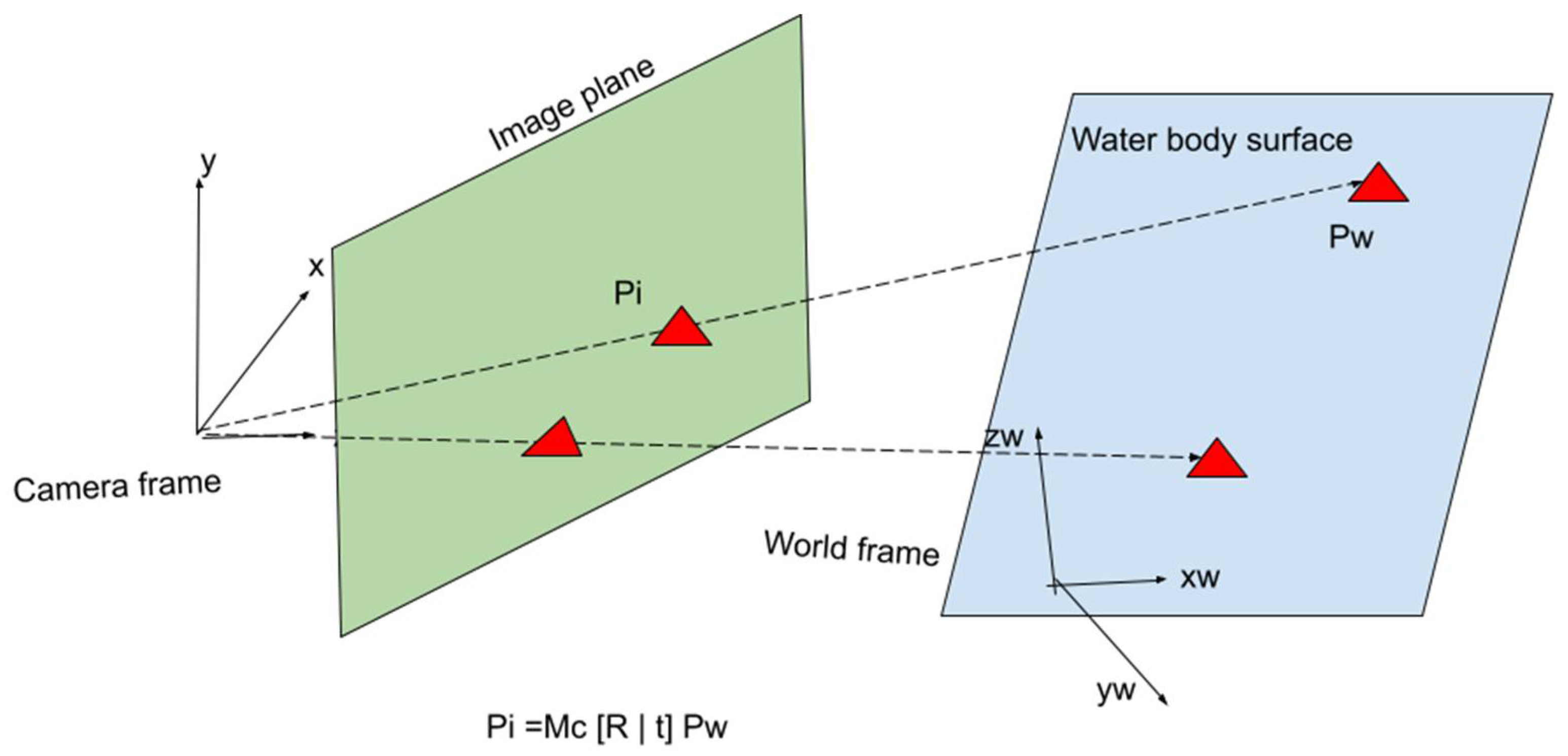
The final step is to convert the corrected 2D bounding box to a 3D coordinate in the reference frame. The problem of solving the 3D world frame coordinates from a 2D bounding box is intractable in general but solvable if additional assumptions are taken to limit the feasible solutions. This process is further broken down into several steps: (1) a proper cameral projection model is selected, (2) the parameters of the camera projection model are estimated, and (3) the estimated model parameters are used in the co-plane projection formulation to calculate the desired target 3D position. Figure 7 illustrates the camera projection of two co-plane objects using a simple camera projection model. The rest of the section will first formulate the 3D projection problem as a parametric estimation problem. We then discuss the co-plane assumption and the derivation of a closed-form 3D solution. $p_i and \widehat{p_i}$ are the observed and reconstructed pixel coordinates in the image plane, and $p_w$ is the corresponding 3D coordinate in the world frame.

Algorithm 2: TF Backward Pass

// p1: likelihood threshold, d1: distance threshold

for anchor[i] in Anchornodes:

for label[j] = pick one uncertain box of a prev frame

if prob(i,j) > p1

label[i] = TARGET

if dist_box(j, i) < d1 // a matching object that is nearby

conf[j] = conf_h

append box[j] to AnchorNodes

5.1. Simple Camera Projective Model

To fully describe a projection model, the intrinsic and extrinsic parameters of the camera are required to compute the transformation matrix. The extrinsic parameters consist of the pose of the camera in the world frame, which is a 6D vector ${\zeta }_e=(x_0, y_0, z_0, \theta , \varphi , \psi )$. The external parameter ${\zeta }_e$ is equivalent to a 3 × 4 transformation matrix for perspective projection.

$$[R |t]=R_x{R}_y{R}_z\left[\begin{array}{ccc}1& 0& 0 x_0\\ 0& 1& 0 y_0\\ 0& 0& 1 z_0\end{array} \right]=\left[\begin{array}{ccc}{r}_{11} r_{12}& r_{13}& rc{w}_1\\ r_{21} r_{22}& r_{23}& rc{w}_2\\ r_{31} r_{32}& r_{33}& rc{w}_3\end{array}\right]$$

Here, $R$ is the rotation matrix and $t=[x_0, y_0, z_0]$ is the translation vector. Typically, $R$ is also expressed as the product of three rotational matrices for the x, y, and z-axes, denoted by $R_x, R_y, R_z$. The intrinsic parameters ${\xi }_{in}=(c_x, c_y, f)$ include the focal length $f$ and the offset of the principle point $c_x, c_y$. The corresponding camera projection matrix is

$$M_c=\left[\begin{array}{ccc}f& 0& c_x\\ 0& f& c_y\\ 0& 0& 1\end{array}\right]$$

Given the camera parameter and the homogenous coordinate of a point in the world frame $P_w=\left(X_{w, }{Y}_w, Z_w, 1\right)$, the forward projection calculates the corresponding pixel location $\widehat{p_i}=\left(u,v\right)$ in the image plane (Figure 7) as follows:

$$\widehat{p_i}=M_{c }[R | t] P_w$$

(1)

The combined nine parameters ${\xi }_{}=\left({\xi }_e, {\xi }_{in}\right)$ completely describe the camera projection model and can be estimated when afforded with enough training data. A suitable optimization method such as the Least Square Error or RANSAC can be used to reduce MLE errors. The optimization process searches the parameter space to minimize the projection error in the training dataset.

$$argmi{n}_{{\mathsf{\xi }}_{}}{{\displaystyle \sum }}^{ }{E}_i(x_0, y_0, z_0,\theta , \varphi , \psi ,f,cx,cy,P_w)$$

(2)

For the i-th training pair $\left(\widehat{p_i}, P_w^i\right)$, we define the error function as the Euclidian distance between the predicted pixel coordinate and the true one:

$$E_i\left(x_0, y_0, z_0,\theta , \varphi , \psi ,f,cx,cy, P_w,\right)=\Vert p_i-\widehat{p_i}\Vert$$

(3)

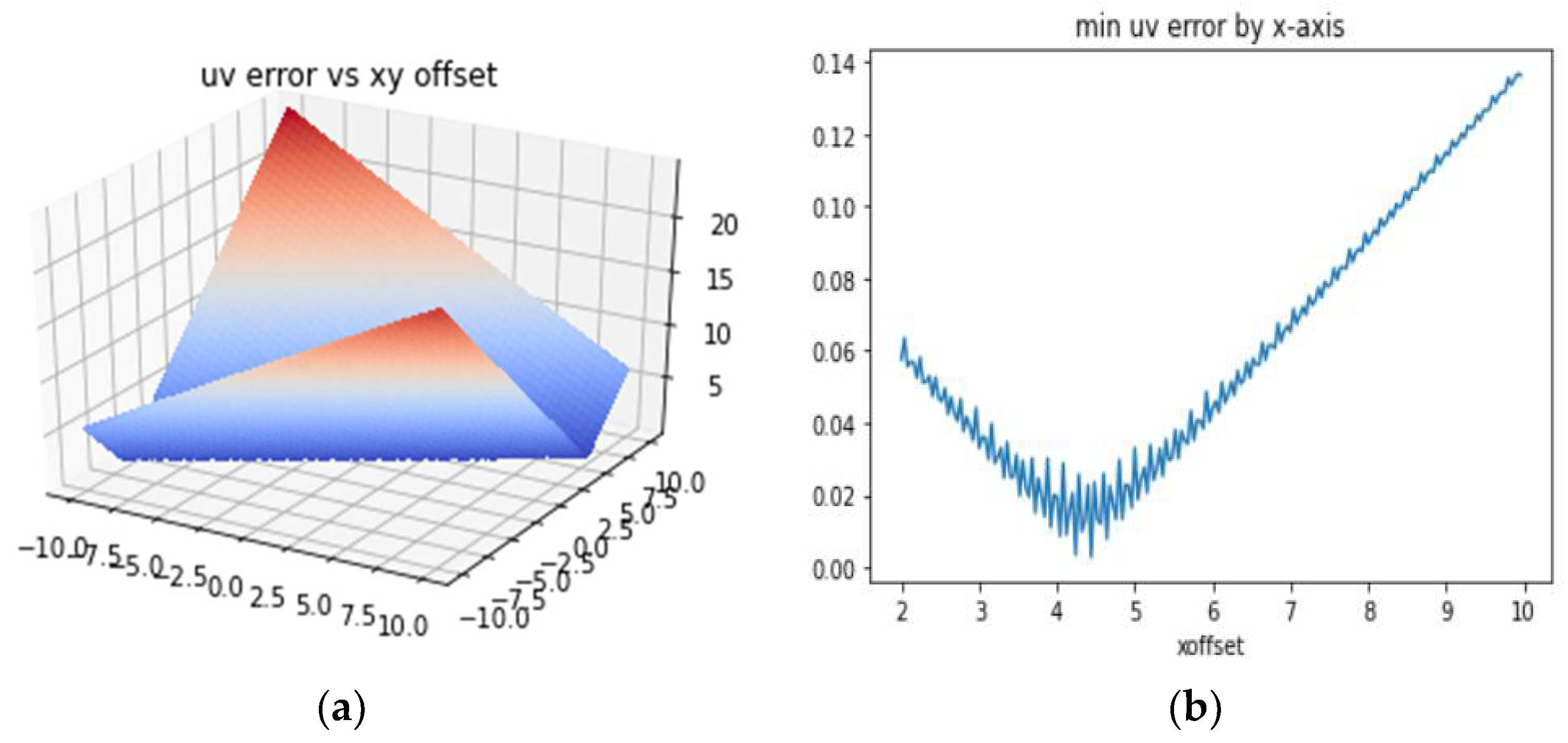
5.2. Piecewise Camera Model Parameter Optimization

In a perfect world, the simple linear camera projection model above should suffice. The parameter optimization problem in (2) can be solved by one of many optimization methods, such as Newton’s gradient descent method. However, the actual dataset in real-world applications might contain image distortion due to lens non-linearity and labeling errors from human mistakes. Furthermore, the training dataset might be distributed unevenly. A single-camera model will not fit all training datasets and will result in significant errors. To tackle this problem, we use a piecewise model consisting of M region-dependent camera models. Let $D_m$ be the domain of the m-th submodel; the piecewise model optimization is formulated as

$$argmi{n}_{{\mathsf{\xi }}_{1\dots M}} {{\displaystyle \sum }}^{ }{E}_m{E}_i(x_0^m, y_0^m, z_0^m,{\theta }^m, {\varphi }^m, {\psi }^m,f^m,cx,cy,P_w)$$

(4)

$$p_i\in {{{\displaystyle \cup }}^{ }}_m{D}_m, D_m=\left(x_l^m,x_g^m\right)\times \left(y_l^m,y_g^m\right)$$

$$D_m{{\displaystyle \cap }}^{ }{D}_n=\varnothing for any m, n$$

The model parameters now consist of the sub-model domain boundaries and the sub-model parameters $\left(x_0^m, y_0^m, z_0^m,{\theta }^m, {\varphi }^m, {\psi }^m,f^m\right)$ for M submodels. The submodel domains are non-overlapping, so membership of the training data point is exclusive to the subdomain. Consequently, at prediction time, a particular sub-model will be selected for prediction for a given data point.

The piecewise parameter search algorithm utilizes a two-step iterative process similar to RANSAC. We first searched for a single-model solution using all ground truth data sets, which are used as an initial solution for all sub-models. We then performed model refinement for each sub-model using only the regionalized ground truth data. The sub-model parameters were then used to adjust the membership of the boundary points for the next iteration. This process is described in the pseudo-code in Algorithm 3.

We simplified the optimization problem by setting the camera frame’s origin to be the camera’s focal point. The origin of the world coordinate frame was set to be the camera origin’s projection point onto the earth seaplane. This effectively forced x₀ = y₀ = 0. Hence, only the vertical translation and the three rotation angles need to be searched.

Algorithm 3: Piecewise Parameter Estimationr (UV[1…n], Pw[1…n])

// input: dataset: UV[]: 2D coordinates, PW[] 3D positions

// output: list of 9-tuple camera parameters: Theta[][9]

Initialize domain boundaries $D_m$

Loop while not converge:

Random adjustment $p_i$ membership using pset[i]

grid[i] = Boundary from trainset[i]

for each grid[i]:

pset[i]= CeresOpt(trainset[i])

// set initial param block

Theta_i= reverse_prjection()

$E_i$ = ||Theta_i − pw_i||

${{\displaystyle \sum }}^{ }{E}_m{E}_i=$ Accumulate errors.

5.3. Co-Plan Reverse Projection to Calculate $P_w$

The co-plane reverse projection based on the estimated camera parameters can now be derived. The input is a 2D position $\widehat{p_i}=\left(u,v\right)$ representing the location of the target in the image domain. The estimated model parameters of the simplified camera model are $\left(z_i, {\theta }_i, {\varphi }_i, {\psi }_i\right)$.

As mentioned earlier, our co-plane assumption is that all target objects are considered to be at the sample plane. This approximation holds for situations such as surface boats, all at sea level. This is also applicable for land robots operating in a relatively flat field. Without loss of generality, we can simplify Equations (1)–(3) by setting $z_w=0$. From the base Equation (1), the expression for $P_C=\left(x_C, y_C,z_C\right)$ is re-written as

$$\begin{gathered} x_C=r_{1,1}{x}_w+r_{1,2}{y}_w+rc{w}_1 \\ {y}_C=r_{2,1}{x}_w+r_{2,2}{y}_w+rc{w}_2 \\ {z}_C=r_{3,1}{x}_w+r_{3,2}{y}_w+rc{w}_3 \end{gathered}$$

(5)

Here, the matrix elements in (1) are derived by inserting the camera parameters into the matrix format. According to the perspective projection matrix, we have

$$\begin{gathered} x_C=u{z}_C \\ {y}_C=v{z}_C \end{gathered}$$

(6)

Combining (5) and (6) after some algebra manipulation leads to

$$\begin{gathered} \begin{array}{c}\left(u{r}_{3,1}-r_{1,1}\right)x_w=\left(r_{1,2}-u{r}_{3,2}\right)y_w+\left(u.rc{w}_3+rc{w}_1\right)\\ \end{array} \\ \left(u{r}_{3,1}-r_{2,1}\right)x_w= \left(r_{2,2}-u{r}_{3,2}\right)y_w+\left(v.rc{w}_3+rc{w}_2\right) \end{gathered}$$

(7)

$$\mathrm{Let} M_r=\left[\begin{array}{cc}u.r_{3,1}-r_{1,1}& u.r_{3,2}-r_{1,2}\\ u.r_{3,1}-r_{2,1}& u.r_{3,2}-r_{2,2}\end{array}\right] \mathrm{and} b_r=\left[\begin{array}{c}u.rc{w}_3-rc{w}_1\\ v.r_{cw3}-rc{w}_{21}\end{array}\right]$$

We obtained the solution to the linear equation in (5) in the world frame coordinate.

$${\left[x_w, y_w\right]}^T=M_r^{-1}\times b_r$$

(8)

Equation (8) calculates the target object’s position in the world frame, given the estimated camera parameters and the object position in the image plane.

6. Experimental Results

6.1. Model Parameter Optimization

The model parameters that minimize the error function in Equation (4) were searched by Algorithm 3. We used the Ceres optimization tool [22] for the sub-model parameter search. To better understand its behavior, we visualized the error function in the (x₀,y₀) subspace in Figure 8. A piecewise sub-model covering a middle-range grid (c = [3, 4]) was used. The error plot showed a noticeable gradient change near the optimum point, a favoring character for the gradient search algorithm. We also observed a gradient valley with many local minima, which might cause some convergence issues. Nevertheless, the Ceres solver seemed to overcome the local minima in our experiments.

The search method was also validated using synthetically generated camera projection data: we randomly selected a block of the camera parameter and fed it with 50 random 3D position points. The 50 pairs of data points were then used by our Ceres solver to produce the estimated model parameters. We observed that the recovered parameters were almost identical to the ground truth. Figure 9 shows the error of the recovered rotational parameters. When optimizing the piecewise model, the boundary of the sub-models is confined such that each grid contain at least 20 data points. The 20-data point threshold is empirically observed for the Ceres solver to converge.

6.2. Position Error with the Field Dataset

We compared the positioning accuracy of the piecewise model and other methods. The two reference methods were the single camera model (marked as Single) and a modified 6DPose method [3]. The single camera method uses the RANSAC method to optimize a single set of parameters $\xi$ over all training data. In our 6DPose implementation, the nueral network was transfer trained with the subset of the RGB images of the boat dataset provided by the NSWC San Diego. Additional 3D box information was labeled to train the 3D net. We focused on the data points where the target boat distances were less than 150 m from the camera. The results are summarized in

Table 1. Average location error predicted by the algorithm, grouped by target distance.

Distance (m)	1–30	30–60	60–90	90–150
Data point	50	50	340	106
Piecewise Model	3.5	5.8	10.2	20.4
Single model	12	16.5	25.3	30.4
6DPose [3]	6.7	8.3	15.0	28.4

. We grouped the results into four target distances from a close to a distant range. The single camera model had the worst position error among the three methods. In particular, the position error of the single camera model increased nearly exponentially as the target distance exceeded 120 m, which justifies the need for a piecewise model. The piecewise model outperformed both the single-camera model and 6DPose method in all distance groups. The 6DPose results are comparative to those of ours for the short distance target. In the practically important 90-m-range target group, the piecewise model had an average error of 10.2 m, and the 6DPose error was 15 m, while the single-camera model had an error of 25.3 m.

6.3. Computing Time

The algorithm run time was evaluated with a desktop computer and an embedded computer. Both platforms have a dedicated GPU to run the YOLO neural network for object detection. The filtering and modal projection were run on the CPU. We point out that Algorithm 3 (model parameter optimization) operates offline, so it did not affect the run time performance at the detection time. The bulk of the computation was spent on object detection and temporal filtering. The calculation of $P_w$ with the optimized camera parameters was negligible.

Table 2. Per-frame processing time comparison on the workstation and TX2. Video resolution: 1024 × 728.

	CPU	GPU	Obj. Detect.	Temp. Filter
Workstation	Intel i-7, 8-core, 3.7 GHz	Titan V 12 GB	6 ms	2 ms
Jetson TX2	Arm-A57, 4-core	8 GB	11 ms	4 ms

shows the breakdown of the algorithm to process each video frame at runtime. On the NVIDIA TX2 platform, the algorithm can process more than 60 frames per second.

6.4. System Robustness

The robustness of the overall system was considered in all three stages of the processing pipeline. At the object detection stage, we initially observed a non-negligible probability of false positives. To improve the correct detection probability, we added multiple object types in training, producing more reliable data and higher confidence in the object bounding boxes. The higher confidence value of the detected 2D bounding box played a significant role in the filtering stage since more anchor nodes could be identified. In the camera parameter optimization stage, a robust system must have stable results against outliers in the training data. The piecewise model design allows outliers to be isolated while optimizing the zone boundaries, and the result showed good tolerance of outliers compared to the other methods.

7. Conclusions

We implemented an ML-aided real-time 3D localization algorithm for co-surface objects solely based on the 2D video input from an RGB camera. Our method uses a deep learning network as the backbone to detect objects and their bounding boxes. To improve the detection success rate for small objects near the horizon, we propose a novel tracking algorithm to correct the detected objects’ classification and the bounding boxes. The tracker identifies anchor frames based on the confidence value of the detected objects and corrects false detections in the initial detection phase. The 2D boxes and the ground truth 3D positions of the target object are then used to train a piecewise camera model to predict target 3D positions. The experimental results showed that the piecewise model outperformed the singular model and a 6DPose-based deep learning method when the ground truth of the training dataset was subject to errors. The location errors of our model were 28% lower than those of both the singular RANSAC-based method and the 6DPose method. The absolute positioning accuracy is less than 10 m for object distances up to 150 m, comparable to that of a GPS. The accuracy is acceptable to support high-level motion planning decisions and collision avoidance for applications such as traffic management in a seaport.