A Hybrid Framework for Lung Cancer Classification
Abstract
:1. Introduction
- A novel hybrid framework LCGANT is proposed to classify lung cancer images and solve the overfitting problem of lung cancer classification tasks.
- The proposed LCGANT framework is better than other state-of-the-art approaches.
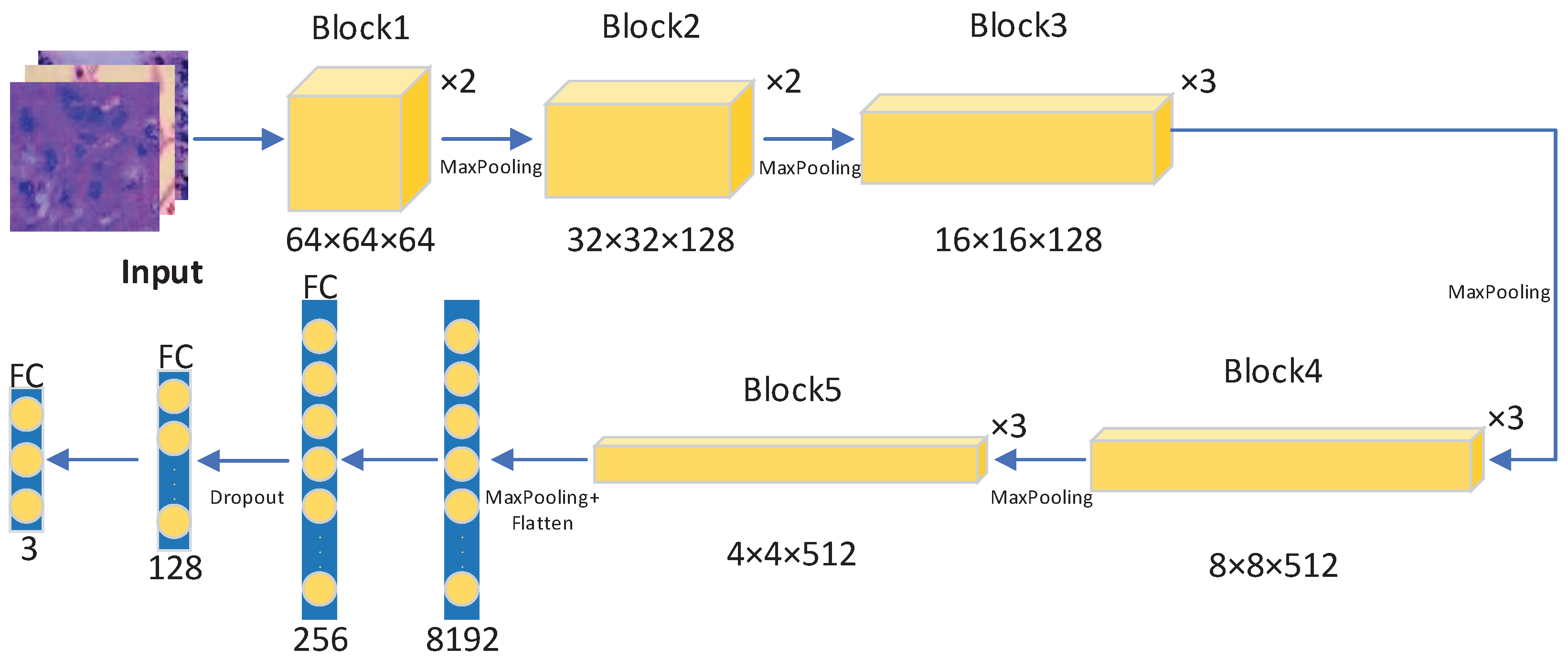
- A lung cancer deep convolutional GAN (LCGAN) can generate synthetic lung cancer datasets to solve lung cancer classification tasks’ limited labelled data issue. A regularization enhanced model called VGG-DF can prevent overfitting problems with pre-trained model auto-selection.
2. Related Work
2.1. Cancer Classification
2.2. Data Augmentation
2.3. Pre-Trained CNN Architecture for Feature Extraction
2.3.1. VGG-16
2.3.2. ResNet50
2.3.3. DenseNet121
2.3.4. EfficientNet
3. Materials and Methods
3.1. Dataset
3.2. Proposed LCGANT Framework for Lung Cancer Classification
3.2.1. Image Synthesis Using LCGAN
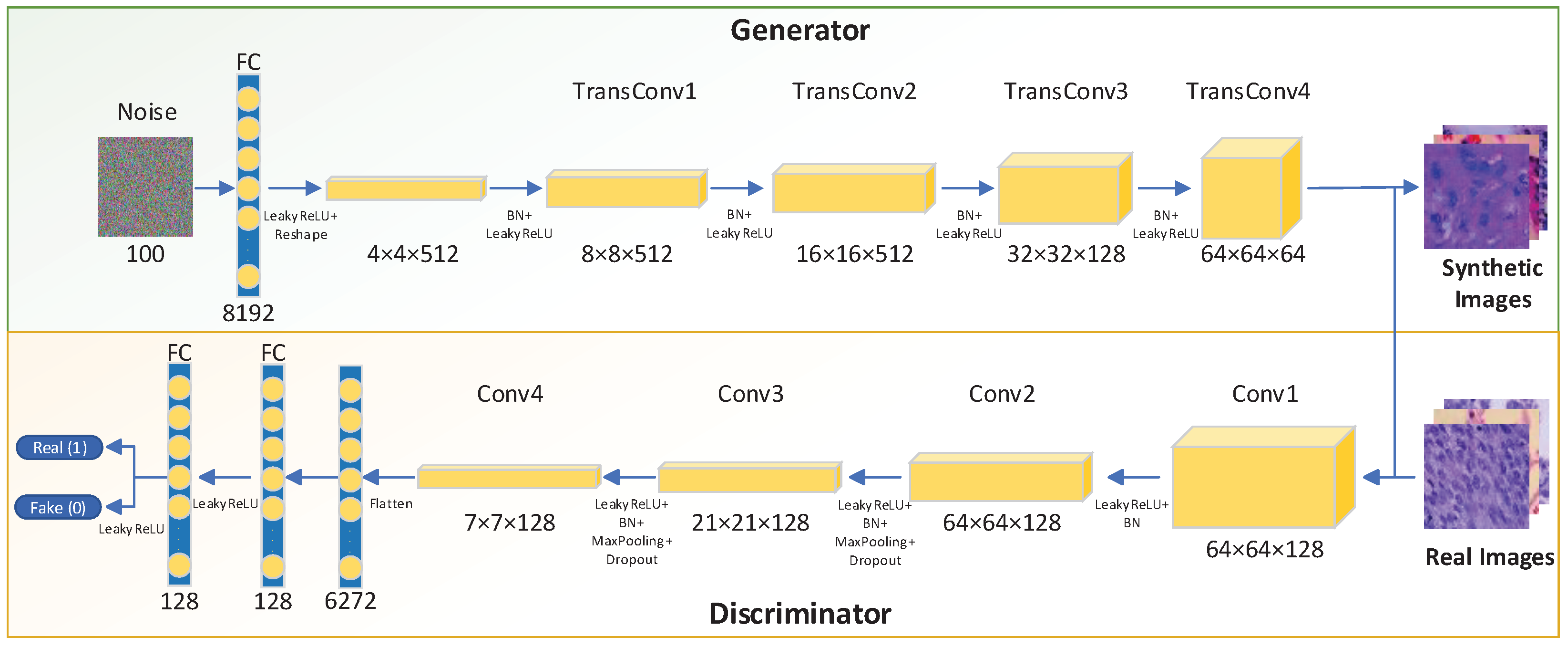
- Replace the fully connected layers with a uniform noise distribution for the generator;
- Use the sigmoid function of the flattened layer for the discriminator;
- Add a Batch Normalization [26] layer to generator and discriminator to avoid poor initialization problems during the training process. The algorithm of Batch Normalization is shown in Equation (2). Here, we use to represent a mini-batch of an entire training set with m examples. Then we can calculate the mean and variance of the mini-batch. Subsequently, we normalize the data in the mini-batch. The is an arbitrarily small constant for numerical stability. Finally, we implement a transformation step to scale and shift the output.
- All layers in the discriminator use the LeakyReLU function.
- Try to add more filters in the front layers of the generator. More filters in the front layers can help the generator to get more activation maps to avoid missing essential features of the original image. Without sufficient filters, the generator will produce blurry images.
- Use the LeakyReLU activation function for all the layers in the generator except the output layer with the Tanh function.
- Add several dropout layers in the discriminator to avoid overfitting.
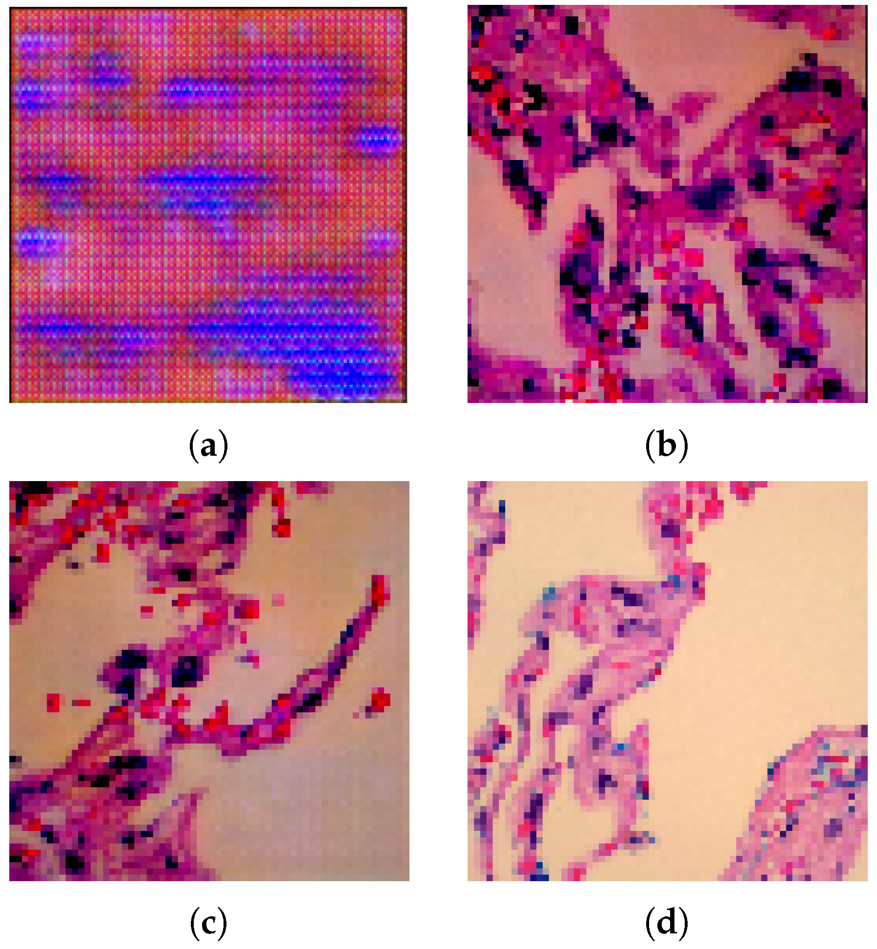
- Avoid checkerboard artefacts:
- During image pre-processing, we use the bilinear interpolation algorithm when we resize the original size to . The bilinear interpolation algorithm is used to do two-dimensional interpolation for a rectangle. First, we find four points of a rectangle: , , , and . Second, we assume the values of four points are for , for , for , and for . Finally, we can estimate the value of the formula at any point . The algorithm can refer to Equation (3).
- Inspired by the idea from [27], the author uses sub-pixel convolution to get a better performance in image super-resolution. Set the kernel size that can be divided by the stride, and try to make the kernel size as big as possible.
3.2.2. Regularization Enhanced Transfer Learning Model
3.2.3. Pre-Trained Model Auto-Selection
4. Results
4.1. Set-Up of Experiments
4.2. Results and Analysis
4.2.1. Lung Images Generated by DCGAN Generator
4.2.2. The Results of Different Transfer Learning Models with Different Training Datasets
4.3. Comparison with State-Of-Art Methods for the Same Dataset
5. Discussion
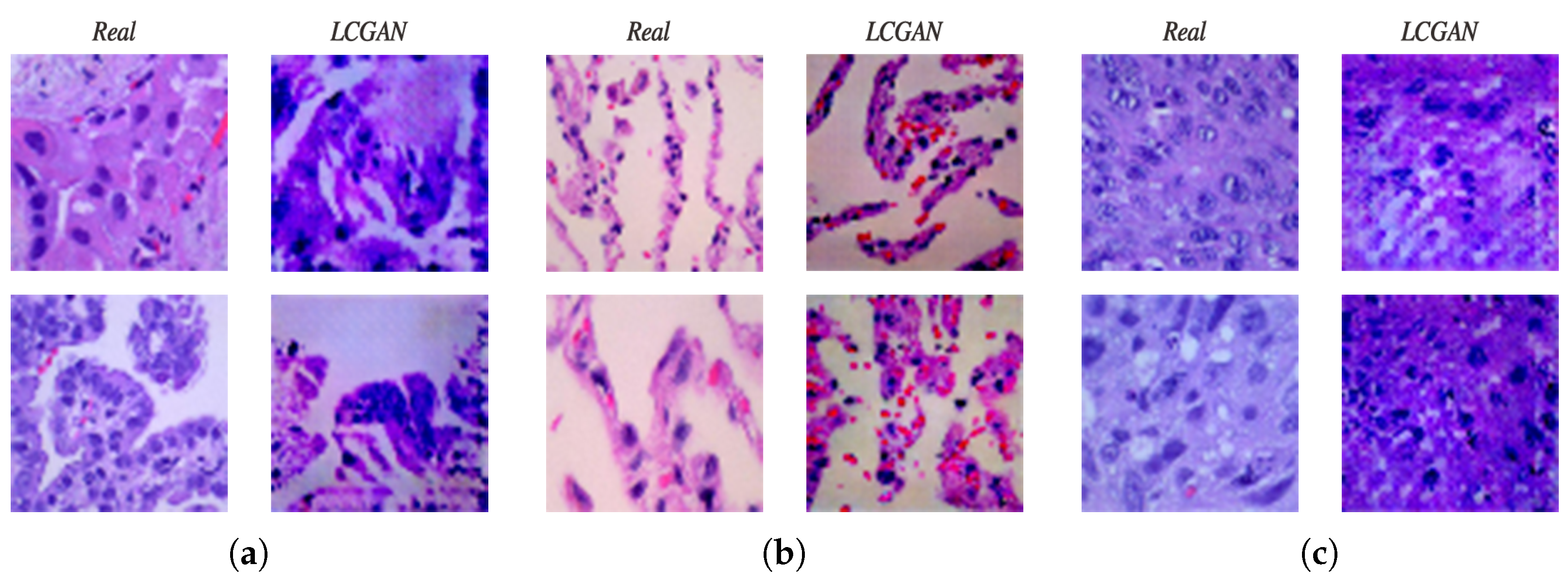
- The synthetic images generated by the LCGAN have slight differences from real images.
- The dimension of images produced by the generator is . This is not sufficient for the biomedical domain. Images with high resolution are very essential in this area.
6. Conclusions
Author Contributions
Funding
Data Availability Statement
Acknowledgments
Conflicts of Interest
References
- World Health Organization. Available online: https://www.who.int/news-room/fact-sheets/detail/cancer (accessed on 9 May 2022).
- Siegel, R.L.; Miller, K.D.; Fuchs, H.E.; Jemal, A. Cancer statistics, 2021. Cancer J. Clin. 2021, 71, 7–33. [Google Scholar] [CrossRef] [PubMed]
- Wernick, M.N.; Yang, Y.; Brankov, J.G.; Yourganov, G.; Strother, S.C. Machine learning in medical imaging. IEEE Signal Process. Mag. 2010, 27, 25–38. [Google Scholar] [CrossRef] [PubMed] [Green Version]
- Alyafeai, Z.; Ghouti, L. A fully-automated deep learning pipeline for cervical cancer classification. Expert Syst. Appl. 2020, 141, 112951. [Google Scholar] [CrossRef]
- Kriegsmann, M.; Haag, C.; Weis, C.A.; Steinbuss, G.; Warth, A.; Zgorzelski, C.; Muley, T.; Winter, H.; Eichhorn, M.E.; Eichhorn, F.; et al. Deep learning for the classification of small-cell and non-small-cell lung cancer. Cancers 2020, 12, 1604. [Google Scholar] [CrossRef] [PubMed]
- Li, J.; Wang, P.; Zhou, Y.; Liang, H.; Luan, K. Different machine learning and deep learning methods for the classification of colorectal cancer lymph node metastasis images. Front. Bioeng. Biotechnol. 2021, 8, 1521. [Google Scholar] [CrossRef]
- Lakshmanaprabu, S.; Mohanty, S.N.; Shankar, K.; Arunkumar, N.; Ramirez, G. Optimal deep learning model for classification of lung cancer on CT images. Future Gener. Comput. Syst. 2019, 92, 374–382. [Google Scholar]
- Perez, L.; Wang, J. The effectiveness of data augmentation in image classification using deep learning. arXiv 2017, arXiv:1712.04621. [Google Scholar]
- DeVries, T.; Taylor, G.W. Dataset augmentation in feature space. arXiv 2017, arXiv:1702.05538. [Google Scholar]
- Goodfellow, I.; Pouget-Abadie, J.; Mirza, M.; Xu, B.; Warde-Farley, D.; Ozair, S.; Courville, A.; Bengio, Y. Generative adversarial nets. Adv. Neural Inf. Process. Syst. 2014, 27, 1–9. [Google Scholar]
- Radford, A.; Metz, L.; Chintala, S. Unsupervised representation learning with deep convolutional generative adversarial networks. arXiv 2015, arXiv:1511.06434. [Google Scholar]
- Mirza, M.; Osindero, S. Conditional generative adversarial nets. arXiv 2014, arXiv:1411.1784. [Google Scholar]
- Zhu, J.Y.; Park, T.; Isola, P.; Efros, A.A. Unpaired image-to-image translation using cycle-consistent adversarial networks. In Proceedings of the IEEE International Conference on Computer Vision, Venice, Italy, 22–29 October 2017; pp. 2223–2232. [Google Scholar]
- Karras, T.; Laine, S.; Aila, T. A style-based generator architecture for generative adversarial networks. In Proceedings of the IEEE/CVF Conference on Computer Vision and Pattern Recognition, Long Beach, CA, USA, 15–20 June 2019; pp. 4401–4410. [Google Scholar]
- Shorten, C.; Khoshgoftaar, T.M. A survey on image data augmentation for deep learning. J. Big Data 2019, 6, 1–48. [Google Scholar] [CrossRef]
- Gatys, L.A.; Ecker, A.S.; Bethge, M. A neural algorithm of artistic style. arXiv 2015, arXiv:1508.06576. [Google Scholar] [CrossRef]
- Zoph, B.; Le, Q.V. Neural architecture search with reinforcement learning. arXiv 2016, arXiv:1611.01578. [Google Scholar]
- Gao, W.; Baskonus, H.M. Deeper investigation of modified epidemiological computer virus model containing the Caputo operator. Chaos Solitons Fractals 2022, 158, 112050. [Google Scholar] [CrossRef]
- Zhong, Y.; Ruan, G.; Abozinadah, E.; Jiang, J. Least-squares method and deep learning in the identification and analysis of name-plates of power equipment. Appl. Math. Nonlinear Sci. 2021. ahead of print. [Google Scholar] [CrossRef]
- Simonyan, K.; Zisserman, A. Very deep convolutional networks for large-scale image recognition. arXiv 2014, arXiv:1409.1556. [Google Scholar]
- Deng, J.; Dong, W.; Socher, R.; Li, L.J.; Li, K.; Fei-Fei, L. Imagenet: A large-scale hierarchical image database. In Proceedings of the IEEE Conference on Computer Vision and Pattern Recognition, Miami, FL, USA, 20–25 June 2009; pp. 248–255. [Google Scholar]
- He, K.; Zhang, X.; Ren, S.; Sun, J. Deep residual learning for image recognition. In Proceedings of the IEEE Conference on Computer Vision and Pattern Recognition, Las Vegas, NV, USA, 27–30 June 2016; pp. 770–778. [Google Scholar]
- Huang, G.; Liu, Z.; Van Der Maaten, L.; Weinberger, K.Q. Densely connected convolutional networks. In Proceedings of the IEEE Conference on Computer Vision and Pattern Recognition, Honolulu, HI, USA, 21–26 July 2017; pp. 4700–4708. [Google Scholar]
- Tan, M.; Le, Q. Efficientnet: Rethinking model scaling for convolutional neural networks. In Proceedings of the International conference on Machine Learning. PMLR, Long Beach, CA, USA, 5–9 June 2019; pp. 6105–6114. [Google Scholar]
- Borkowski, A.A.; Bui, M.M.; Thomas, L.B.; Wilson, C.P.; DeLand, L.A.; Mastorides, S.M. Lung and colon cancer histopathological image dataset (lc25000). arXiv 2019, arXiv:1912.12142. [Google Scholar]
- Ioffe, S.; Szegedy, C. Batch normalization: Accelerating deep network training by reducing internal covariate shift. In Proceedings of the International conference on Machine Learning PMLR, Lille, France, 7–9 July 2015; pp. 448–456. [Google Scholar]
- Shi, W.; Caballero, J.; Huszár, F.; Totz, J.; Aitken, A.P.; Bishop, R.; Rueckert, D.; Wang, Z. Real-time single image and video super-resolution using an efficient sub-pixel convolutional neural network. In Proceedings of the IEEE Conference on Computer Vision and Pattern Recognition (CVPR), Las Vegas, NV, USA, 27–30 June 2016; pp. 1874–1883. [Google Scholar]
- Bukhari, S.U.K.; Asmara, S.; Bokhari, S.K.A.; Hussain, S.S.; Armaghan, S.U.; Shah, S.S.H. The Histological Diagnosis of Colonic Adenocarcinoma by Applying Partial Self Supervised Learning. medRxiv 2020. [Google Scholar]
- Phankokkruad, M. Ensemble Transfer Learning for Lung Cancer Detection. In Proceedings of the 4th International Conference on Data Science and Information Technology, Shanghai, China, 23–25 July 2021; pp. 438–442. [Google Scholar]
- Hlavcheva, D.; Yaloveha, V.; Podorozhniak, A.; Kuchuk, H. Comparison of CNNs for Lung Biopsy Images Classification. In Proceedings of the IEEE 3rd Ukraine Conference on Electrical and Computer Engineering (UKRCON), Lviv, Ukraine, 6–8 July 2021; pp. 1–5. [Google Scholar]
- Masud, M.; Sikder, N.; Nahid, A.A.; Bairagi, A.K.; AlZain, M.A. A machine learning approach to diagnosing lung and colon cancer using a deep learning-based classification framework. Sensors 2021, 21, 748. [Google Scholar] [CrossRef]
- Hatuwal, B.K.; Thapa, H.C. Lung Cancer Detection Using Convolutional Neural Network on Histopathological Images. Int. J. Comput. Trends Technol 2020, 68, 21–24. [Google Scholar] [CrossRef]
- Chehade, A.H.; Abdallah, N.; Marion, J.M.; Oueidat, M.; Chauvet, P. Lung and Colon Cancer Classification Using Medical Imaging: A Feature Engineering Approach. 2022. preprint. Available online: https://assets.researchsquare.com/files/rs-1211832/v1_covered.pdf?c=1641239335 (accessed on 6 April 2022).
- Raza, K.; Singh, N.K. A tour of unsupervised deep learning for medical image analysis. Curr. Med. Imaging 2021, 17, 1059–1077. [Google Scholar] [CrossRef] [PubMed]


| Hyperparameter | Value |
|---|---|
| Optimizer | Adam |
| Loss (LCGAN) | Binary Crossentropy |
| Loss (VGG-DF) | Categorical Crossentropy |
| Dropout Probability | 0.2 |
| Batch Size | 256 |
| Number of Epochs (LCGAN) | 15,000 |
| Number of Epochs (VGG-DF) | 5 |
| Kernel Size (G) | 4 |
| Kernel Size (D) | 3 |
| Layer (Type) | Output Shape | Number of Parameters |
|---|---|---|
| Input | 100 | 0 |
| Dense | 8192 | 827,392 |
| LeakyReLU | 8192 | 0 |
| Reshape | 0 | |
| TransConv | 4,194,816 | |
| BatchNorm | 2048 | |
| LeakyReLU | 0 | |
| TransConv | 2,097,408 | |
| BatchNorm | 1024 | |
| LeakyReLU | 0 | |
| TransConv | 524,416 | |
| BatchNorm | 512 | |
| LeakyReLU | 0 | |
| TransConv | 131,136 | |
| BatchNorm | 256 | |
| LeakyReLU | 0 | |
| TransConv | 3075 | |
| Activation | 0 | |
| Total Parameters: 7,782,083 | ||
| Trainable Parameters: 7,780,163 | ||
| Non-trainable Parameters: 1920 | ||
| Layer (Type) | Output Shape | Number of Parameters |
|---|---|---|
| Input | ||
| Conv2D | 3584 | |
| LeakyReLU | 0 | |
| BatchNorm | 512 | |
| Conv2D | 147,584 | |
| LeakyReLU | 0 | |
| BatchNorm | 512 | |
| MaxPooling | 0 | |
| Dropout | 0 | |
| Conv2D | 147,584 | |
| LeakyReLU | 0 | |
| BatchNorm | 512 | |
| Conv2D | 147,584 | |
| LeakyReLU | 0 | |
| BatchNorm | 512 | |
| MaxPooling | 0 | |
| Dropout | 0 | |
| Flatten | 6272 | 0 |
| Dense | 128 | 802,944 |
| LeakyReLU | 128 | 0 |
| Dense | 128 | 16,512 |
| LeakyReLU | 128 | 0 |
| Dense | 1 | 129 |
| Total Parameters: 1,267,969 | ||
| Trainable Parameters: 1,266,945 | ||
| Non-trainable Parameters: 1024 | ||
| VGG-DF (Ours) | ResNet50 | DenseNet121 | EfficientNetB4 | |
|---|---|---|---|---|
| Accuracy | 95.80% | 95.56% | 53.87% | 45.96% |
| Precision | 95.81% | 95.56% | 76.86% | 75.93% |
| Sensitivity | 95.80% | 95.56% | 53.87% | 45.96% |
| F1-score | 95.80% | 95.56% | 49.62% | 38.44% |
| VGG-DF (Ours) | ResNet50 | DenseNet121 | EfficientNetB4 | |
|---|---|---|---|---|
| Accuracy | 99.84% | 99.46% | 79.64% | 51.74% |
| Precision | 99.84% | 99.49% | 66.81% | 68.70% |
| Sensitivity | 99.84% | 99.46% | 59.19% | 51.74% |
| F1-score | 99.84% | 99.46% | 52.06% | 43.03% |
| Reference | Model (Method) | Accuracy | Precision | Sensitivity | F1-Score |
|---|---|---|---|---|---|
| [28] | RESNET50 | 93.91% | 95.74% | 81.82% | 96.26% |
| RESNET18 | 93.04% | 96.81% | 84.21% | 95.79% | |
| RESNET34 | 93.04% | 95.74% | 80.95% | 95.74% | |
| [29] | Ensemble | 91% | 92% | 91% | 91% |
| ResNet50V2 | 90% | 91% | 90% | 90% | |
| [30] | CNN-D | 94.6% | - | - | - |
| [31] | DL-based CNN | 96.33% | 96.39% | 96.37% | 96.38% |
| [32] | CNN | 97.2% | 97.33% | 97.33% | 97.33% |
| [33] | XGBoost | 99.53% | 99.33% | 99.33% | 99.33% |
| Our method | LCGANT | 99.84% | 99.84% | 99.84% | 99.84% |
Publisher’s Note: MDPI stays neutral with regard to jurisdictional claims in published maps and institutional affiliations. |
© 2022 by the authors. Licensee MDPI, Basel, Switzerland. This article is an open access article distributed under the terms and conditions of the Creative Commons Attribution (CC BY) license (https://creativecommons.org/licenses/by/4.0/).
Share and Cite
Ren, Z.; Zhang, Y.; Wang, S. A Hybrid Framework for Lung Cancer Classification. Electronics 2022, 11, 1614. https://doi.org/10.3390/electronics11101614
Ren Z, Zhang Y, Wang S. A Hybrid Framework for Lung Cancer Classification. Electronics. 2022; 11(10):1614. https://doi.org/10.3390/electronics11101614
Chicago/Turabian StyleRen, Zeyu, Yudong Zhang, and Shuihua Wang. 2022. "A Hybrid Framework for Lung Cancer Classification" Electronics 11, no. 10: 1614. https://doi.org/10.3390/electronics11101614
APA StyleRen, Z., Zhang, Y., & Wang, S. (2022). A Hybrid Framework for Lung Cancer Classification. Electronics, 11(10), 1614. https://doi.org/10.3390/electronics11101614


