Modeling of the Crystallization Conditions for Organic Synthesis Product Purification Using Deep Learning

Abstract

Crystallization is an important purification technique for solid products in a chemical laboratory. However, the correct selection of a solvent is important for the success of the procedure. In order to accelerate the solvent or solvent mixture search process, we offer an in silico alternative, i.e., a never previously demonstrated approach that can model the reaction mixture crystallization conditions which are invariant to the reaction type. The offered deep learning-based method is trained to directly predict the solvent labels used in the crystallization steps of the synthetic procedure. Our solvent label prediction task is a multi-label multi-class classification task during which the method must correctly choose one or several solvents from 13 possible examples. During the experimental investigation, we tested two multi-label classifiers (i.e., Feed-Forward and Long Short-Term Memory neural networks) applied on top of vectors. For the vectorization, we used two methods (i.e., extended-connectivity fingerprints and autoencoders) with various parameters. Our optimized technique was able to reach the accuracy of 0.870 ± 0.004 (which is 0.693 above the baseline) on the testing dataset. This allows us to assume that the proposed approach can help to accelerate manual R&D processes in chemical laboratories.

1. Introduction

Crystallization is used as a purification technique for solids, and it is one of the fundamental procedures based on the principles of solubility [1,2]. Crystallization as a purification technique is mostly applicable not only in the laboratory but also in industry as a tool to obtain pure components from various mixtures (organic–inorganic chemical reactions, plant extracts, etc.) [3]. Solutions are cooled to a point where they become suspensions, or anti-solvents are added to induce the process. The solid is removed from the suspension, which hopefully results in a purer form of the solute. The developing crystals ideally form with high purity, while impurities remain in the saturated solution surrounding the solid [4]. The crystallized solid is then filtered away from the impurities [5]. This effect is achieved because the solvent can no longer hold all of the solute molecules, and they begin to leave the solution and form solid crystals. Chemists use laboratory techniques to purify solid compounds [6], and the focus of this paper is on how to help them by transferring some of these processes from a real into an artificial environment.

An important feature of crystallization is the selection of an appropriate solvent. The solubility of a compound depends on the solvent(s) and their ratios, the temperature, the pH of the system, the presence of impurities, and the solid form in equilibrium with the supernatant [7]. Synthetic crystallization process design often relies on the understanding of solubility in order to isolate the compound as a solid with the polymorphic form of interest at a high yield while limiting the presence of impurities within the isolate. The solvent used in a crystallization experiment is often critical to obtaining the best results. The most common methods of selection are based on prior knowledge or the compound’s similarity to a known appropriate solvent [8]. However, the selection of crystallization solvents for novel compounds remains costly because it requires testing in the experimental laboratory [9]. The high cost is usually due to the expensive expert labor and materials.

In practical terms, a methodology that would allow the approximation of the crystallization solvents may allow scientists to predict what solvents they would need to use for the purification step before even starting the synthesis. Thus, this paper aims to offer a reasonable approach which is able to predict an appropriate solvent (or several solvents) (from the pre-determined closed set of possible solvents) for the purification of synthesis mixtures using crystallization. Most notably, modern Machine Learning (ML) algorithms, in particular Deep Learning (DL), have demonstrated an unparalleled ability to model various chemical properties [10]. In this research, we use a novel training dataset that was prepared for this purpose and contains various organic syntheses, but does not bind to a specific reaction type. The input data (containing reactants and products) is presented in the SMILES (Simplified molecular-input line-entry system) notation. We test the two most promising vectorization types (extended-connectivity fingerprints and autoencoders) and two types of neural networks (i.e., a Feed-Forward Neural Network—FFNN and Long Short-Term Memory—LSTM) as classifiers. In addition, we investigate whether the knowledge of the solvent mixture before the crystallization step is necessary in order to achieve a higher accuracy of prediction. This research assumes that the correctly chosen methodology (vectorization type, classifier, hyper-parameters) can solve the solvent selection problem in silico first, before transferring its outcomes to a real chemistry laboratory. This could ease the scouting of appropriate crystallization solvents, leading to increased efficiency and solvent savings.

2. Related Work

Purification by crystallization is one of the most popular operations in the laboratory and industry [11,12,13]. Although methods for the selection of potential solvents for crystallization and recrystallization have been researched [14], the process is still challenging, especially when the solubility is not determined for novel compounds. Besides this, the purification of laboratory chemicals using crystallization remains labor-intensive [15].

The selection of a suitable candidate for the crystallization step is accomplished by several methods discussed in this paragraph. The most trivial is candidate selection by looking up similar documented reaction procedures [16]. Computational screening technologies have been developed to circumvent costly experimental screening and reduce wastage in the development of crystallization processes. The more complicated methods are computer-aided: they are based on a generic formulation for the design of a crystallization solvent system. A framework is used to determine the optimal system of organic solvents and a case study for ibuprofen is illustrated in [17]. Other methods employ a framework for the design of crystallization solvents, and CAMD (single compound and mixture) is used to design optimal solvents and their systems [18].

Supervised ML (SML) has been relied upon by scientists to solve various problems in the field of chemistry. The important branch of SML, i.e., DL (deep learning), has become one of the most prominent method groups that can deal with high-dimensional and complex data. In contrast to simple computer programs, where calculations follow an explicit set of instructions, SML-based systems rely on models trained on “gold” (i.e., manually prepared, undisputed, correct) examples (i.e., inputs and related outputs). The learning process produces a model that approximates the input–output relationships. Chemistry data are notorious for complex relationships between the input (usually molecules) and the desired output (which ranges from simple descriptors to synthetic routes). One of the critical issues is the proper selection of the molecular representation, i.e., features. However, typically a molecule is represented by a linear form or by a graph-like network of atoms, which is called SMILES. Despite this, SML methods cannot be directly applied to SMILIES. Hence, a SMILES string has to be further converted into different formats such as molecular descriptors, fingerprints, one-hot encoding, or word embedding. The molecule itself contains diverse information, such as individual atoms, their connections, types of bonds between atoms, spacial configurations, and so on. Probably the simplest molecular vectorization solution is one-hot encoding [19]. Similarly, for every molecule, various descriptors can be calculated, such as the molecular weight and Wiener index, etc. [20]. Descriptors have been successfully used in artificial intelligence-aided drug design research [21]. A more sophisticated vectorization approach—in particular, extended-connectivity fingerprints (ECFP) that calculate features of molecules based on atom neighbors—has been used to predict reaction outcomes [22,23]. However, state-of-the-art vectorization method types used with Artificial Neural Networks (ANNs) have been implemented to represent structures in latent space with the use of auto-encoders [24,25]. For example, a variational autoencoder (VAE) that is trained solely on molecular representations is a good representative of it. While most molecular representation-based models require prior curation and feature engineering, a VAE can rapidly learn these representations from SMILES strings directly, without prior manipulation. The VAE takes the form of a “bowtie”-shaped ANN. In the middle of this network is a “bottleneck layer” or latent vector into which inputs are mapped, represented as a vector of numbers (encoding) with a reverse process (decoding) seeking to return the SMILES string presented as the input [26]. Conditional variational auto-encoders have been used with an ANN for molecular design, to control molecular properties. However, in these algorithms, the degrees of freedom are limited and property control is difficult to achieve. In [27], a molecular generative model based on the conditional VAE is proposed, which has degrees of freedom that enable the easy control of multiple properties simultaneously. As a proof of concept, it can be used to generate drug-like molecules with five target properties: Molecular Weight (MW), LogP, hydrogen bond donor (HBD), hydrogen bond acceptor (HBA) numbers, and topological polar surface area (TPSA). Authors have demonstrated how to generate drug-like molecules with specific values for the five target properties within an error range of 10%.

Applications of ML in chemistry have become increasingly popular in recent years [28]. ML techniques have received great attention in the field of chemistry, especially in organic chemistry. These techniques are used to predict drug targets and side effects, new molecular structures, chemical reactions, and properties. However, the replacement of rule-based algorithms with SML is not straightforward due to the enormous chemical space size (10⁶⁰ molecules) of synthetically feasible molecules (<500 Da) [29]. Data quantity has always been one of the key issues over the last decade of ML and chemistry research. Even including the ~60 million compounds produced over the last century, the coverage would be microscopic compared to the entire chemical space [30]. However, more does not necessarily mean better: different tasks often require only the most relevant data. Besides this, even seemingly limited datasets did not hinder scientific progress in the field of AI-driven chemistry. Tasks such as drug discovery [31,32,33], the prediction of chemical properties [34,35], and the prediction of reaction yield have been successful at delivering promising results [36]. It has been experimentally demonstrated that small datasets can be used to produce meaningful results with the help of transfer learning, especially in areas where the collection of data is challenging [37].

ANNs are a subset of ML methods with great potential to have an arbitrarily selected network topology and to perform nonlinear transformations of their inputs. While intermediate ANN layers can vary in numbers, forms, and connectivity, the input must always be a numeric tensor. The group of ANNs covers a broad range of different ANN types, topologies, and values of hyper-parameters. FFNNs have been successfully used to predict drug-likeness for central nervous system drugs [38]. Another type of ANN is a Convolutional Neural Network (CNN), which supports convolution operations that take advantage of the spatial 2D structure of input data. In other words, a convolutional layer uses filters to apply a dot product between its inputs and the filter’s weights. Molecules in drug discovery tend to be small molecules; as such, they are represented as atomic-type descriptors. The research offers a method that extracts descriptors of the atomic type, distance, coordinate position, and other information according to the molecular characteristics, and uses it to construct a multi-channel grid-based CNN for toxicity prediction. The experimental investigation proves that the offered method outperforms other convolution ML methods, including DL [39]. Similar research also relies on the CNN with the SMILES linear notation of compounds. The feature matrix was designed and applied to CNN in the way that the convolution operation is performed only in one direction along the SMILES string. The performance of the CNN based on the SMILES string was superior to the conventional fingerprint method used for the virtual screening of chemical compounds [40]. However, CNN methods are a rather rare option compared to other alternatives, such as Recurrent Neural Networks (RNN). The prediction of physical properties is a widely studied area for ML scientists [41,42,43]. In one of the studies, a trained LSTM model was used for sequence processing. Both the embedded channel attention and spatial attention modules are identically critical factors for the prediction of properties from the SMILES sequence. Experimental results showed that the trained model is capable of providing highly reliable predictions for aqueous solubility [44]. Moreover, RNNs have also enabled researchers to generate de novo molecules [45,46,47]. Research in [48] describes a methodology for the de novo design of bioactive compounds employing RNNs trained on a large dataset of bioactive molecules. This bidirectional (BIMODAL) network model can generate diverse bioactive compounds with high chemical validity, which provide highly valuable scaffolds for prospective drug discovery investigations. Few other ML studies have been undertaken so far, even though the solvation mechanism for non-aqueous solutions plays an important role in various chemical reactions. The ML-based QSPR (quantitative structure property relationships) method, Delfos (DL model for solvation free energies in generic organic solvents), can effectively predict solvation free energies for various organic solute and solvent systems. Delfos was designed from two separate solvent and solute encoder networks that can quantify the structural features of given compounds via word embedding and recurrent layers, augmented with an attention mechanism which extracts important substructures from outputs of RNNs. This model offers a promising framework for the accurate prediction of complex molecular interactions between chemical compounds in a wide range of applications, including material development, drug design, and more [49]. As mentioned before, LSTM networks can cope with sequences, and have therefore been used for drug discovery: DL is used to predict the binding of a molecule to a possible target receptor [50]. Another novel approach [51], i.e., the Controlled Molecule Generation (CMG) method, can optimize a molecule property by utilizing BiLSTM (Bidirectional LSTM). CMG takes advantage of the self-attention-based molecule translation model and two constraint networks, which are pre-trained separately. The two constraint networks can effectively regulate the output molecules by regularizing the activations computed in the molecule translation model. The offered approach also takes advantage of a BiLSTM which is capable of processing the input sequence flow in both directions, i.e., forward and backward. It helps to consider the context not only from the past but from the future.

General-purpose hybrid DL methods are another group of approaches that typically consist of multiple interacting nonlinear elements, and each of these elements may be an ANN, a linear discriminant, or an arbitrary model with no apparent connection to ANNs or statistical discriminants. Hybrid methods have also proven to be effective. An example of one is the trained DL model for drug side-effect prediction and description, consisting of a graph CNN with Inception modules, and a BiLSTM word-embedding layer [52]. The GCNN is used to predict drug relationships by autoencoding drug names that are converted into word vectors via the word-embedding layer. The CNN module extracts drug molecular properties from the graphs, which are then fed into the BiLSTM to predict drug side effects in the correct flow of interpretable descriptive language. Comparisons with other baseline models show that the hybrid model achieves a superior AUC prediction score and robustness.

To summarize, the computational methods employed in the field of cheminformatics vary widely based on the solving task; therefore, different methods have to be tested in order to achieve optimal results. Based on the available research, we decided to test the two most promising vectorization types (ECFP and ECFP autoencoders) and two types of neural networks (FFNN and LSTM) as classifiers. We hypothesize that a method for the prediction of a suitable solvent system for crystallization can be created directly from information about the reactants and products. In practice, the resulting mixture of chemicals right after the reaction has occurred might require an in-depth analysis with analytical instruments. In this case, the trained neural network would be able to approximate the most suitable solvent based on the reaction that occurs within the mixture, and could infer the byproducts. This semi-automatic method allows us to predict the optimal solvent compositions in advance, which may significantly reduce the number of assay experiments and accelerate the discovery process. It may allow scientists to predict the most suitable solvent system without the problematic analysis of the reaction mixture and the manual modeling of compound systems. This, in turn, would facilitate R&D processes within the laboratories, and would lead to the rapid development of novel compounds or an earlier launch of successful drugs on the market.

Our major contribution in this paper is a novel method for the prediction of solvent systems directly from the reactants and products for crystallization. The modeling of such solvent systems that are invariant to the reaction type has not been previously demonstrated. In addition, the approximation of solvent systems for the purification of chemical reaction mixtures has not been thoroughly researched. The findings in our research open up new horizons for more complex and universal models based on DL in the field of chemistry and informatics. Furthermore, we publish two new datasets, used in our work, for further research in this field.

3. Formal Definition of a Solving Task

In this research, we solve the solvent label prediction problem of the crystallization procedure. We denote the chemical reaction as d_i that belongs to a space of chemical reactions d_i ∈ D. Each d_i can be converted into a p-dimensional feature vector X_i = (x_i,1, x_i,2, …, x_i,p), which serves as an input.

Let Y = {y₁, y₂, … y_N} be an N-sized space of class labels (in our case, it is a closed-set of possible solvents), which represent the output. Let η be a mapping function η(X) → Y which, for each input, can predict a subset of solvent labels.

Let Γ be an ML algorithm that could learn an approximation (denoted as η’) of function η from the training dataset D^L ⊂ D. The goal of Γ is to learn which model is able to predict, as accurately as possible, the class labels from their inputs automatically on the testing dataset D^T, D^T= D − D^L. The D^L and D^T datasets are not overlapping (D^L ∩ D^T = ∅), and both have enough diversity and are correctly distributed in the space. If both of these conditions are met, the evaluation results will be considered reliable.

4. The Data

The subset from Daniel Mark Lowe’s and NextMove’s open-source collection of chemical reactions extracted from the US patents issued from 1976–2016 was used to create the dataset for our ML algorithms [53]. The original (full) dataset contains 3.7 million reactions and synthesis procedures. Each reaction is represented by a unique action sequence (or recipe) describing the steps taken in the laboratory to derive the final product. All of the synthesis procedures are divided into separate actions taken in the laboratory; for example, the addition of a reactant, the heating of the reaction mixture, filtration, extraction, and crystallization, etc. From the original dataset, a custom-made script extracted only our solving task-related samples, and later restructured them to become suitable for the prediction of the solvent names used in the crystallization step of the syntheses. During the dataset cleaning process, a few noticeable outliers were removed. Our created dataset has two versions: the first one (noted as DS1) contains information about the chemical reactants, products, and the solvents used in crystallization; the second (DS2) is identical to the first one but is complemented with the additional information about the solvents in the mixture before crystallization.

Instances in both versions (DS1 and DS2) are chemical reactions represented as sequences of symbols describing reactants and products’ chemical structures. The SMILES representation is used to denote the graph-like structure of each molecule [54]. Such a form of molecule representation consists of alphanumeric characters without embedded whitespace that encode the topology of the graph as well as any other atom properties. Individual molecules are separated with the “.” dot symbol, while reactants, catalysts and reactants are separated with “>>” symbols, in that order. Table 1 contains snippets from DS1 and DS2, both containing a sequence of molecules in SMILES notation as inputs. The snippets are presented in order to show the difference between DS1 and DS2, with the former containing pre-crystallization solvent information as part of an input to the neural networks along with the compounds. The table also presents the solvents used for the crystallization procedure.

Table 1. Snippet from our dataset (compounds, solvents in the mixture before crystallization, and solvents used for the crystallization procedure are shown).

Name	Compounds	Pre-Crystallization Solvents	Solvent (Prediction)
DS1	OC=O.CC(C)N(C(CN)=O)c1ccccc1>>Cc1ccccc1>>CC(C)N(C(CNC=O)=O)c1ccccc1	Toluene	Hexane
DS2	Nc1cccc(O)c1.N#Cc1cccc([N+]([O-])=O)c1C#N>>Nc1cccc(Oc(cc2)cc(C#N)c2C#N)c1	-	Pyridine

Both the DS1 and DS2 datasets contain 180,145 shuffled instances (d_i) split into subsets for training (90%, 162,131 instances) and testing (10%, 18,015 instances). Each instance has a maximum of two labels, with ~1.28 labels on average per instance. The closed-set contains 13 class labels in total that have been used as solvents or anti-solvents for crystallization (Hexane, Ethyl acetate, Ethanol, Ether, Methanol, Acetonitrile, Isopropanol, Water, Toluene, Acetone, DCM, Chloroform, DMF). The most covered are Hexane, Ethyl acetate, and Ethanol. The classes were chosen from the original dataset if there were enough instances to have sufficient representation of the class label. An extremely rare class label with a low number of instances would not contribute to an overall increase of the accuracy and practical value. Table 2 illustrates the distribution of instances over different labels.

Table 2. Distribution of instances over different class labels (DS1 and DS2).

Class Label	Training Subset (Number of Instances)	Testing Subset (Number of Instances)	Total (Number of Instances)
Hexane	42,421	4713	47,134
Ethyl acetate	41,983	4665	46,648
Ethanol	31,658	3518	35,175
Ether	21,975	2442	24,417
Methanol	18,796	2088	20,884
Acetonitrile	8398	933	9331
Isopropanol	7227	803	8030
Water	5612	624	6236
Toluene	4930	548	5478
Acetone	3874	430	4304
DCM	3704	412	4115
Chloroform	1815	202	2017
DMF	1765	196	1961
Total number of instances	162,131	18,015	180,145

The trained models’ results will be compared to random (Equation (1)) and majority (Equation (2)) baselines. A random baseline represents the boundary that the accuracy must exceed for the method not to be considered as the random labeler. A majority baseline represents the probability of the major class, i.e., the accuracy that would be achieved if all instances would be automatically attached to the largest class. Thus, both random and majority baselines must be exceeded in order for the method to be considered suitable for our solving task.

$$Random baseline={{\displaystyle \sum }}_{i=1}^n\left(P{\left(y_i\right)}^2\right)$$

(1)

n—number of classes, (P(y_i))—the probability of y_i class.

$$Majority baseline=\max \left(P\left(y_{largest}\right)\right)$$

(2)

The calculated random and majority baselines for both datasets are equal to 0.096 and 0.177, respectively.

The only major difference between DS1 and DS2 is that DS2 has additional information about which solvents (of the 31 possible) were in the reaction mixture before the crystallization step. Their labels are THF, Water, DCM, DMF, Ethanol, Methanol, Toluene, Ethyl acetate, Acetic acid, Acetonitrile, Pyridine, Dioxane, Chloroform, Acetone, Benzene, Ether, DMSO, Triethylamine, Isopropanol, HCl, Hexane, NaOH, Dichloroethane, Dimethyl sulfoxide, Xylene, Carbon tetrachloride, Trifluoroacetic acid, Sulfuric acid, 1,2-dimethoxyethane, N, N-dimethylacetamide, Formic acid. Each sample has ~1.3 solvent labels on average.

All of the reactants and products of the reaction are combined into a sequence: reactant 1, reactant 2, reactant 3, etc. However, the ANN must be trained to ignore the positions of reactants. Due to this, the datasets were augmented by permuting molecules randomly of every given instance. However, the dataset augmentation process was restricted to avoid the exponential growth of instances by limiting the maximum number of permutations to 8. This was done on purpose: too many “cloned” instances (that do not have variety in the content) would negatively impact the training process by overflooding and prolonging it.

5. Materials and Methods

5.1. Vectorization

The symbol lines that represent chemical structures in SMILES notation are not suitable for supervised machine-learning algorithms. The input data must be transformed into a matrix of numeric values. We have selected two vectorization methods:

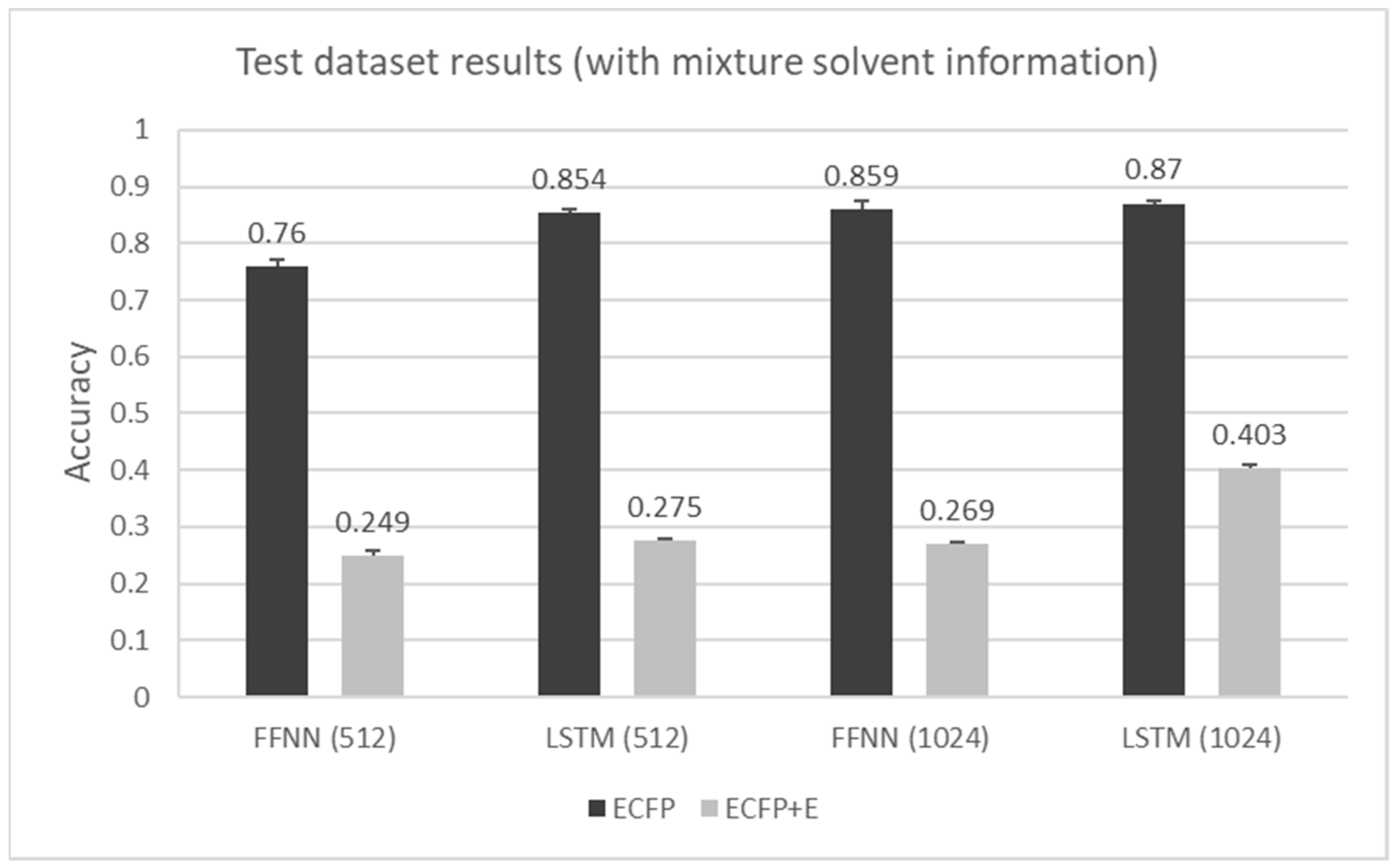
• Extended-connectivity fingerprints (ECFP) that can capture representations of molecular structures [55]: ECFPs are based on the Morgan algorithm, and are commonly used in such applications as virtual screening or ML [56]. ECFPs denote the absence or existence of specific substructures by scanning atom neighbors. The vectorization method works by transforming each molecule into a binary vector (containing zeros and ones) of a chosen length. In our experiments, we tested 512 and 1024 lengths of vectors. Because an instance in the dataset is multiple reactants, the vectors are combined into a matrix.
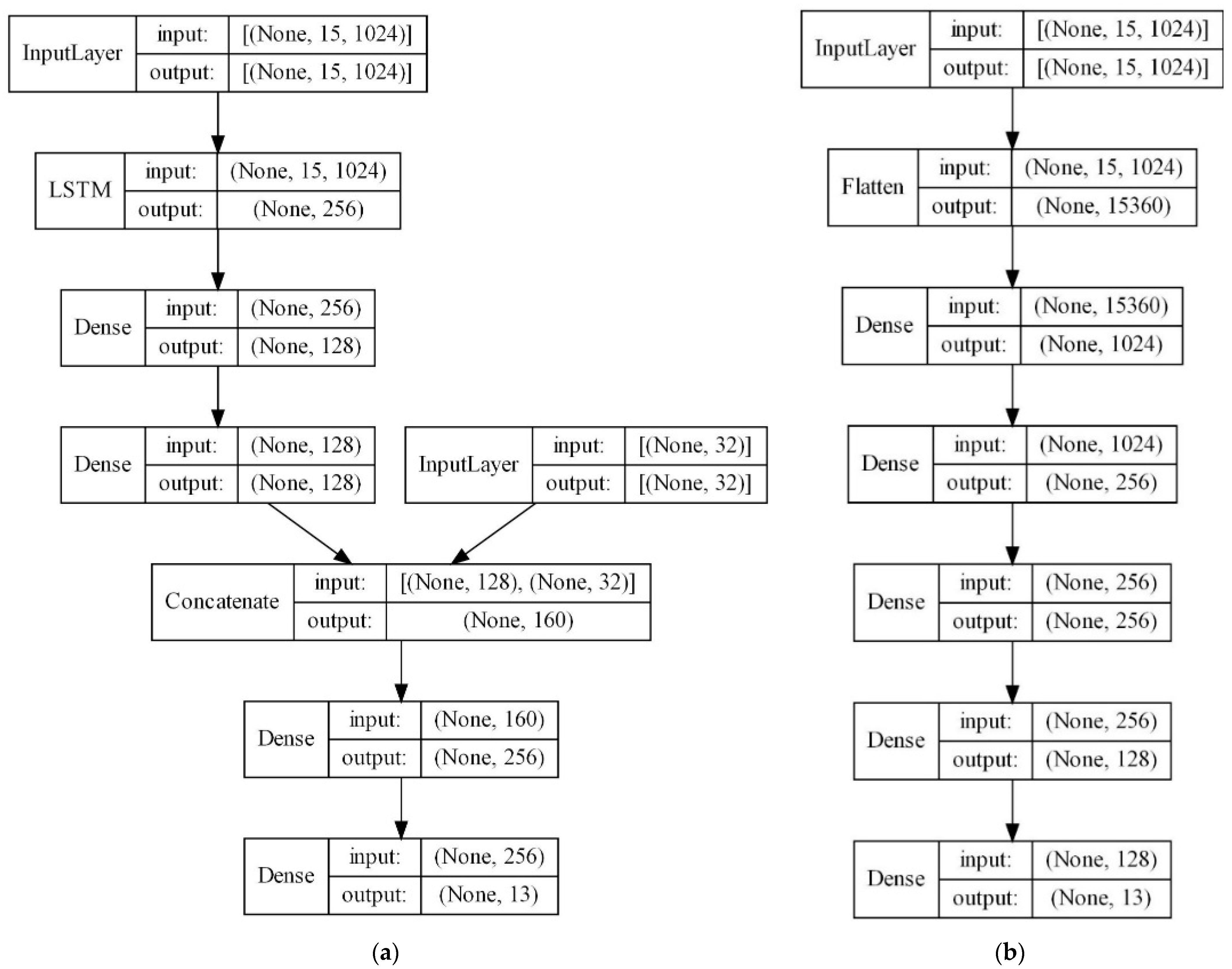
• ECFP encoders (ECFP + E): Autoencoders can be effective in reducing dimensionality for sparse matrices, such as ECFP. The main advantage of autoencoders is that they are trained in an unsupervised manner (they do not require labeled data). Additionally, autoencoders can learn the principal components, i.e., the created model can capture important patterns while ignoring the noise. This technique is often utilized in information retrieval, text analysis, and recommender systems. An autoencoder is trained to take in ECFPs and reproduce identical ECFPs in the output layer. The middle layer, the so-called bottleneck layer, is smaller than the input; therefore, the network must learn to compress the input data in a meaningful way [57]. Encoder weights are learned separately, but later can be used as the “starting point” of the deeper ANN architecture for different downstream tasks (e.g., solvent labeling, as in our case). The main advantage is that encoders may learn how to map sparse inputs to a denser latent space, which results in the detection of relevant parts, and often leads to higher accuracy.

During this research, we have investigated different auto-encoder types (i.e, FFNN and LSTM), topologies, and hyperparameters. Lengths of 512 and 1024 ECFP vectors were tested; therefore, two auto-encoders were trained for each type of ANN. The main parameter of auto-encoders is the latent dimension size, which was set to 512 and 1024, with 512 and 1024 vectors, respectively. These values were not chosen accidentally: they produced the most accurate reproductions and compressed the input data by 15 times (because the input matrix is 512 × 15 or 1024 × 15). Besides this, different latent dimension sizes were tested by stacking multiple neural network layers containing 64, 128, 256, 512, 1024, and 2048 neurons; however, shallow auto-encoders performed better, and were selected for the final testing. Figure 1 illustrates the topologies and sizes of the layers of FFNN- and LSTM-based auto-encoders. The encoders were later combined with an FFNN classifier.

Figure 1. FFNN (a) and LSTM (b) encoders.

5.2. Supervised Machine-Learning Approach

DL is a group of state-of-the-art ML approaches which are able to approximate the relationships between input and output data. In recent years, DL has been effectively applied to a variety of research fields, including computer vision, natural language processing, and drug discovery. The ability of DL to identify complex patterns in datasets has been a major driving force behind the growth of this field. However, the performance of DL models significantly depends on the solving task, type/completeness/diversity of the dataset, and other important factors. Modeling the relationship between chemicals and the corresponding crystallization solvent system is difficult, due to the large variety of possible molecules and the complex interactions between them.

Different types of ANNs have been developed; however, we focused only on the most suitable ones for our solving task:

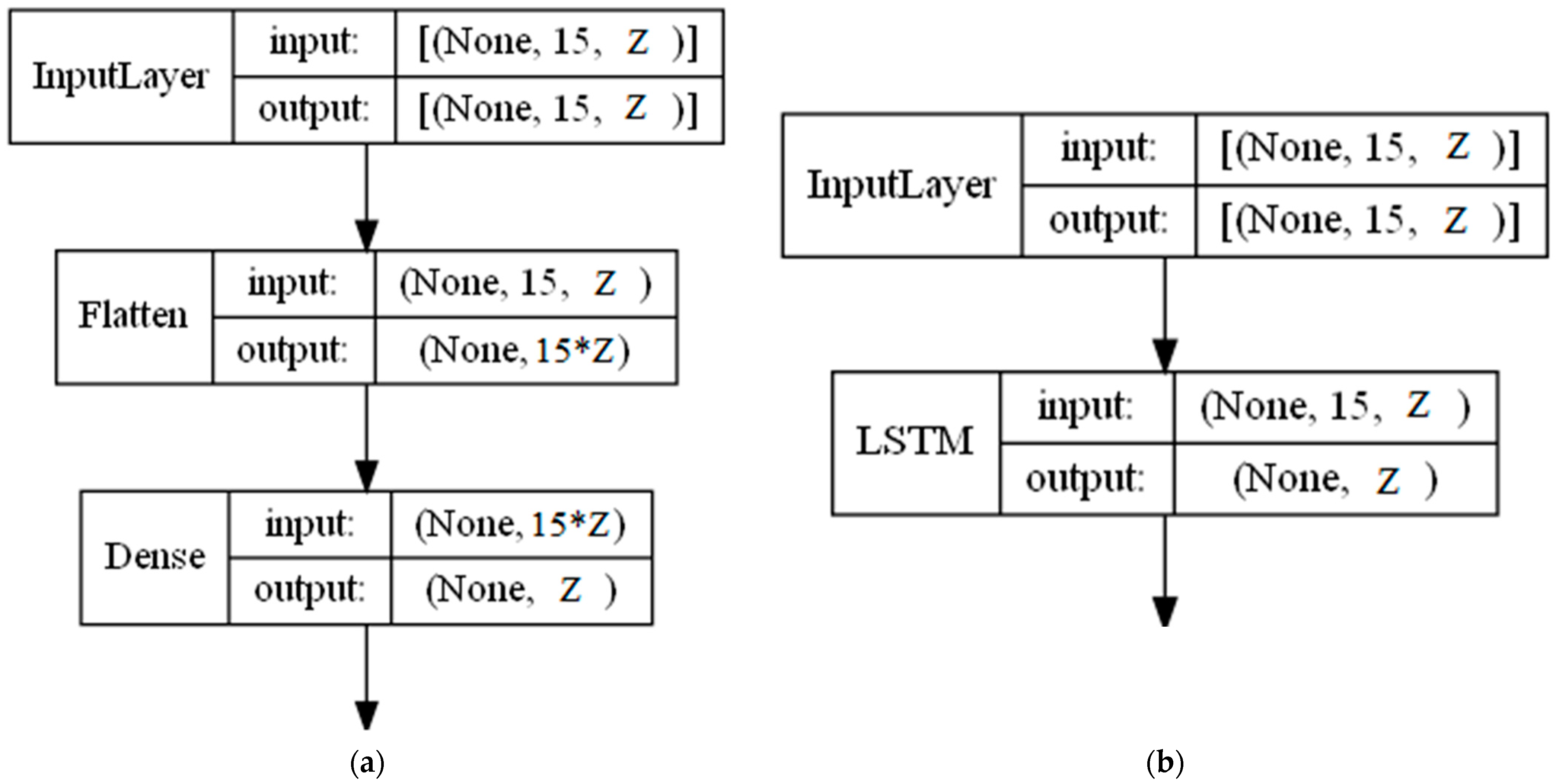
• A Feed-Forward Neural Network (FFNN) is an ANN in which the information flows through different layers, but only in one direction, i.e., forward. In its feed-forward, non-recurrent structure, the input is passed through the layers of nonlinearities or neurons (Logistic Sigmoid or Hyperbolic Tangent) until it reaches the output. The number of nodes in the input layer corresponds to the number of predictors (independent variables) from the dataset, and the number of nodes in the output layer corresponds to the number of response classes. FFNN is a simple network that can be trained faster than other networks; besides this, it usually serves as a baseline approach.
• Long Short-Term Memory (LSTM) is an ANN that can learn long-term dependencies between time steps of sequence data. LSTMs work well even when the input or output sequences are long (e.g., hundreds or thousands of time steps long), and can capture both long-term and short-term trends in the input sequence. The sigmoid function is used to control how much of each input or output is kept or forgotten across different time steps. The forget gate controls which information has to be removed from this layer’s state. Meanwhile, the input and output gates determine what information from the current time step and carryover information from previous time steps has to be combined to produce this layer’s output at the current time step. Considering the nature of the chemical molecules with significant parts in the structure, it is important to notice that, from the theoretical perspective, LSTMs should be the most suitable option for our solving task.

Hyper-parameters play an important role in the model training process as well; therefore, we have investigated them together with the large variety of values:

• Activation functions: Activation functions in ANN are important because they introduce non-linearity into the network. Without activation functions, ANNs would be limited to representing only linear models of data. They also determine whether a neuron should be activated or not by calculating the “weighted sum” and later adding bias to it. In this research, we tested several activation functions: GELU [58], SELU [59], ReLU, ELU, and tanH. The ReLU activation function is commonly chosen because it can be quickly computed, and therefore the model converges quickly, which is useful if training multiple models, and in optimization. GELU, SELU, and ELU are nonlinear modifications of ReLU. The last ANN’s layer’s activation function depends on the type of the solving task. We chose the sigmoid activation function because it is the only compatible function with the binary cross-entropy loss function used for loss calculation. The output vector contains multiple independent binary variables, and the sigmoid function returns the corresponding values in the range (0–1).
• The optimizer is also an important hyper-parameter that controls the training process. The Adam optimizer is probably the most popular choice due to its ability to effectively control the learning rate, and due to its high speed compared to other methods, such as Stochastic Gradient descent (SGD). The classic gradient descent algorithm is an iterative method of finding the minimum of a function. Starting from a random point on the function, the gradient descent algorithm follows the slope down towards the minimum value of that function. At each step, the gradient descent algorithm updates its current position based on the learning rate and loss of a given point plus momentum [60]. Nadam and Adamax optimizers that are modifications of the Adam algorithm were also tested.
• The batch size and the number of training epochs are both important hyperparameters. The batch size determines how many samples can be sent to the network for a single update iteration. The number of training epochs determines how many times the entire dataset is passed to the network. It is important to evaluate your results after each epoch in order to determine whether the model is overfitting or still underfitting the data. The batch size and the number of training epochs are both significant parameters that affect the training process overall. A larger batch size is usually beneficial, as it may prevent overfitting because the model is forced to approximate larger batches of instances. Multiple tests have shown that the most optimal batch size is 128. The number of epochs depends on the batch size. Once the optimal batch size is found, most of the models will have have successfully converged at epoch 25 or before. Typically, the training process is monitored and terminated if the accuracy metric is no longer improved. A binary cross-entropy loss function was used for loss calculation, as the output vector contains multiple independent binary variables.

5.3. Optimization

The main goal of our solving task is to optimize the model’s parameters. The optimization process for an ANN is monitored using the weights and biases platform for ML developers. Before training multiple ANN models and testing their topologies, ranges or lists of parameter values are defined. After every training epoch, a validation dataset is used to evaluate the model’s performance. The weights and biases platform tracks logs, such as the loss function value, as well as model outputs, such as the predictions made by the model on the validation dataset. The weights and biases platform also visualizes hyper-parameters vs. performance, which allows an efficient search for the optimal values of hyper-parameters that improve the model performance without overfitting on the training data (i.e., without memorizing or overfitting). In our experiments, we investigated 16 unique combinations of neural network types, vectorization types, vector sizes, and whether there is information about a mixture before the crystallization step. All of the combinations are enumerated and presented in Table 3.

Table 3. Combinations the neural network types, vectorization types, vector sizes, and whether there is information on a mixture before the crystallization step.

Number	Neural Network Type	Vectorization	Vector Size	Pre-Mix Info
1	FFNN	ECFP	512	no
2	LSTM	ECFP	512	no
3	FFNN	ECFP	1024	no
4	LSTM	ECFP	1024	no
5	FFNN	ECFP	512	yes
6	LSTM	ECFP	512	yes
7	FFNN	ECFP	1024	yes
8	LSTM	ECFP	1024	yes
9	FFNN	ECFP + E	512	no
10	LSTM	ECFP + E	512	no
11	FFNN	ECFP + E	1024	no
12	LSTM	ECFP + E	1024	no
13	FFNN	ECFP + E	512	yes
14	LSTM	ECFP + E	512	yes
15	FFNN	ECFP + E	1024	yes
16	LSTM	ECFP + E	1024	yes

During the model tuning phase, the following parameters were optimized:

• Neural network layer size: 16, 32, 64, 128, 256, 512, and 1024 neurons
• Activation functions: GELU, SELU, ReLU, ELU, and tanH
• Optimizers: Adam, Nadam, SGD, and Adamax
• Batch sizes: 32, 64, 128, 256, 512, and 1024

Next to the parameter tuning, different ANN architectures were investigated by varying the numbers of layers: layers were added or removed depending on whether this increased the model’s performance. During this process, the metrics of the validation dataset were constantly monitored in order to evaluate the model’s performance. The layers were added until the evaluation metrics improved. This iterative process lasted until the metrics were stabilized. The two models that were able to achieve the highest accuracy are illustrated in Figure 2. The optimal models’ parameters for each combination are also presented in the Github repository: https://github.com/Mantas-it/crystall_neuralmodelling (accessed on 30 March 2022).

Figure 2. Topologies of the two optimal models that resulted in the highest accuracy (with an additional input for pre-crystallization solvents (a) and without the same (b)).

6. Results

The following experiments were performed on two versions of the dataset (described in Section 4), using two vectorization methods (in Section 5.1) and two classifiers (in Section 5.2). For this purpose, the Python 3.7 (Guido van Rossum, Netherlands, Amsterdam) programming language with the TensorFlow Keras API library was used.

As presented in Section 3, we solved the multi-label classification task; in order to evaluate it, we chose Accuracy (Equation (3)), Precision (Equation (4)), Recall (Equation (5)), and F1-score (Equation (6)) metrics.

In Equations (3)–(6), TP (true positive) denotes the number of cases when y_i was correctly predicted as y_i; TN (true negative) denotes the cases when y_j was correctly predicted as y_j; FP (false positive) denotes incorrect cases when y_j was predicted as y_i; FN (false negative) denotes incorrect cases when y_i was predicted as y_j.

$$Accuracy=\frac{TP+TN}{TP+FP+TN+FN}$$

(3)

$$precision=\frac{TP}{TP+FP}$$

(4)

$$Recall=\frac{TP}{TP+FN}$$

(5)

$$F1score=\frac{2\times precision\times recall}{precision+recall}$$

(6)

The experiments with two vectorization methods (ECFP, ECFP + E), two classifiers (FFNN, LSTM), two vector lengths (512 and 1024), and two versions of the dataset (with solvent mixture information and without) were performed. Each experiment was repeated three times; the results were averaged, and the confidence intervals (with a confidence level of 95%) were calculated. The obtained accuracies are visually presented in Figure 3 and Figure 4; for more detailed results (including the Precision, Recall, and F1-score values) see Table 4 and Table 5.

Figure 3. Visual representation of the accuracy values on DS1.

Figure 4. Visual representation of the accuracy values on DS2.

Table 4. Evaluation results on DS1. The lengths of the vectors are presented in parenthesis.

Vectorization	Metric	FFNN (512)	LSTM (512)	FFNN (1024)	LSTM (1024)
ECFP	Accuracy	0.617 ± 0.003	0.832 ± 0.008	0.836 ± 0.004	0.836 ± 0.004
	Precision	0.842 ± 0.005	0.899 ± 0.006	0.847 ± 0.008	0.905 ± 0.004
	Recall	0.689 ± 0.003	0.877 ± 0.004	0.759 ± 0.008	0.880 ± 0.006
	F1-score	0.758 ± 0.004	0.888 ± 0.005	0.800 ± 0.002	0.892 ± 0.002
LE	Accuracy	0.267 ± 0.005	0.257 ± 0.006	0.371 ± 0.006	0.862 ± 0.003
	Precision	0.576 ± 0.007	0.655 ± 0.012	0.568 ± 0.003	0.928 ± 0.011
	Recall	0.354 ± 0.005	0.336 ± 0.013	0.502 ± 0.007	0.889 ± 0.002
	F1-score	0.439 ± 0.005	0.444 ± 0.009	0.533 ± 0.003	0.908 ± 0.006
ECFP + E	Accuracy	0.617 ± 0.003	0.832 ± 0.008	0.836 ± 0.004	0.836 ± 0.004
	Precision	0.842 ± 0.005	0.899 ± 0.006	0.847 ± 0.008	0.905 ± 0.004
	Recall	0.689 ± 0.003	0.877 ± 0.004	0.759 ± 0.008	0.880 ± 0.006
	F1-score	0.758 ± 0.004	0.888 ± 0.005	0.800 ± 0.002	0.892 ± 0.002

Table 5. Evaluation results on DS2. The lengths of the vectors are presented in parenthesis.

Vectorization	Metric	FFNN (512)	LSTM (512)	FFNN (1024)	LSTM (1024)
ECFP	Accuracy	0.617 ± 0.003	0.832 ± 0.008	0.836 ± 0.004	0.836 ± 0.004
	Precision	0.842 ± 0.005	0.899 ± 0.006	0.847 ± 0.008	0.905 ± 0.004
	Recall	0.689 ± 0.003	0.877 ± 0.004	0.759 ± 0.008	0.880 ± 0.006
	F1-score	0.758 ± 0.004	0.888 ± 0.005	0.800 ± 0.002	0.892 ± 0.002
LE	Accuracy	0.267 ± 0.005	0.257 ± 0.006	0.371 ± 0.006	0.862 ± 0.003
	Precision	0.576 ± 0.007	0.655 ± 0.012	0.568 ± 0.003	0.928 ± 0.011
	Recall	0.354 ± 0.005	0.336 ± 0.013	0.502 ± 0.007	0.889 ± 0.002
	F1-score	0.439 ± 0.005	0.444 ± 0.009	0.533 ± 0.003	0.908 ± 0.006
ECFP + E	Accuracy	0.617 ± 0.003	0.832 ± 0.008	0.836 ± 0.004	0.836 ± 0.004
	Precision	0.842 ± 0.005	0.899 ± 0.006	0.847 ± 0.008	0.905 ± 0.004
	Recall	0.689 ± 0.003	0.877 ± 0.004	0.759 ± 0.008	0.880 ± 0.006
	F1-score	0.758 ± 0.004	0.888 ± 0.005	0.800 ± 0.002	0.892 ± 0.002

7. Discussion

Zooming into the results presented in Table 3 and Table 4, Figure 2 and Figure 3 allow us to state that all of the tested methods are suitable for our solving task because they significantly exceed the random (0.096) and majority (0.177) baselines.

Unfortunately, the direct comparison of our obtained results to any previously reported results is impossible because (1) the solvent prediction problem (formulated as the multi-label supervised classification problem) has not been solved before with the automatic ML methods, and (2) we have used a specifically created training dataset (by selecting relevant instances from the D. M. Lowe’s dataset) that was used to train the solvent prediction model directly from reactants and products. However, for these two reasons, the performed research is interesting from a scientific point of view.

Because the direct comparison of our results with previously reported results is not possible, we compared them—at least—to some traditional ML approaches, in particular Naïve Bayes. This approach was selected on purpose: the Naïve Bayes assumption about the feature independence allows parameters to be learned separately, it performs especially well when there are a lot of equally significant features, and the method is fast and does not require huge data storage resources. Due to all these reasons, it is often selected as the baseline approach. The tested Naïve Bayes method for our dataset resulted in 0.255 ± 0.017 accuracy. Despite it having demonstrated superiority over the random and majority baselines, Naïve Bayes failed significantly compared to our optimal offered methodology.

In this research, we tested two vectorization techniques (ECFP, ECFP + E) and two classifiers (FFNN and LSTM). The optimal configuration on the DS2 was having necessary information about the solvents before crystallization for the vectorization technique, and the classifier was ECFP (vector length = 1024) and LSTM, respectively: it reached the accuracy of 0.870 ± 0.004. The second-best result (0.862 ± 0.004 accuracy) achieved on DS1 (i.e., without any information about the solvents before crystallization) was again the LSTM classifier that was applied on top of ECFP + E (length = 1024). LSTM cells can remember important information for longer periods of time, and are vitally important for the interpretation of chemical symbol sequences. Hence, these results demonstrate the impact of the prior information about the solvents before crystallization: it can slightly boost the performance. Despite this, the increase was insignificant (by 0.008), and therefore allowed us to conclude that this prior information (that sometimes is very difficult to get) is not mandatory. Thus, the optimal results can be achieved either with or without additional knowledge.

The vectorization with ECFP seems to be the optimal choice with all of the tested configurations (all versions of the datasets, classifiers, and their parameters), except for ECFP + LSTM on DS1. However, the ability of ECFP + E to cope with some tasks is also not accidental: it was proven to be a good option when predicting chromatographic solvent systems in [61]. Despite this, it is important to emphasize that ECFP + E typically requires more training compared to ECFP to achieve similar accuracy levels. This limitation might become an obstacle in cases when large amounts of training data are not available. Our solving task is also interesting from this perspective because the training dataset is not enormously huge (compared to what is typically used when training very accurate ANN-based models); therefore, the superiority of ECFP is reasonable. Although our recommendation for similar tasks regarding the vectorization type is clear, the level of compression (i.e., vector size) in the latent layer is very task-dependent, and therefore might need adjustments.

In contrast to what we assumed before the experimental investigation, the length of the fingerprints does have a significant impact on the prediction accuracy: the longer ones (of 512 and 1024) allowed models to achieve higher accuracy levels. Besides this, in our preliminary experiments (that were not very comprehensive, and therefore were not presented in his paper) it was noted that very short lengths (<64) restrict the model from proper training, which results in its low accuracy even below random and majority baselines. These insights allow us to claim that longer fingerprints may lead to optimal results.

The FFNN classifier underperforms LSTM in various configurations, achieving 10–20% higher accuracy. The explanation of this phenomenon lies in the nature of these methods. Simple FFNN ignores complex relations (treating them as separate features) between fingerprints in molecules. On the contrary, LSTM can process sequential data, and can combine individual molecular fingerprints in a meaningful manner.

Overall, optimized methods have achieved reasonably high accuracy (considering all of the evaluation metrics presented in the paper). Besides this, multi-labeled cases were considered accurate only if all of the solvents were predicted correctly, which means that we have applied a stricter assessment method. However, in the majority of the tested and erroneously considered instances, at least one solvent label was predicted correctly. This means that the accuracy is even higher. Because we want to use our method in real chemistry laboratories (that place very high demands on the accuracy of in-silico methodology), semi-correct predictions had to be disregarded and considered to be false. The accuracy is also sensitive to noise in the training dataset. Although much manual effort was made to ensure the correct labeling of reactions and solvent labels, the collected data span a few decades of organic chemistry research, meaning that not every single example within the dataset contains the optimal choice for crystallization. Despite our efforts to clean the dataset, it still may contain some noisy examples: automatically performed dataset pre-processing cannot avoid errors completely. Even knowing that the training dataset is not of the gold standard, the achieved accuracy is promising. Despite this, the following steps must cover the detailed error analysis, the constant search for more training data of good quality, and further methodology improvements. The implementation of all of these listed steps is in our nearest plans.

8. Conclusions and Future Work

In this paper, we offered reasonable approaches based on modern ML (i.e., DL) algorithms to predict appropriate solvents for the purification of synthesis mixtures using crystallization. We tested two vectorization methods (ECFP and ECFP encoders) along with two types of neural networks (FFNN and LSTM) on two versions of datasets (with and without prior knowledge about the solvents in the mixture before crystallization).

The optimal configuration (reaching the accuracy of 0.870 ± 0.004) was composed of the ECFP vectorization technique and the LSTM multi-label classifier. Besides this, it was achieved on the dataset containing additional information (i.e., information about the solvents before crystallization). The results significantly exceed the majority and random baselines, equal to 0.177 and 0.096, respectively. However, if the prior knowledge about the solvents before crystallization is not given, then LSTM applied on the ECFP + E is the better option. The high achieved accuracy suggests that our offered methodology may be applied in practice, and to accelerate R&D processes in real chemical laboratories.

In the future, we are planning to continue our investigation in several directions: (1) by testing a larger variety of ANN types, such as BiLSTM and transformer models; (2) by increasing the number of solvents used in the crystallization process by extending the number of classes and their coverage by training instances; and (3) by testing the offered methodology in real chemical laboratories, and by investigating the level of practicality by using tools functioning according to our offered methodology.

References

- Erdemir, D.; Lee, A.Y.; Myerson, A.S. Nucleation of Crystals from Solution: Classical and Two-Step Models. Acc. Chem. Res. 2009, 42, 621–629. [Google Scholar] [CrossRef]
- Weng, J.; Huang, Y.; Hao, D.; Ji, Y. Recent Advances of Pharmaceutical Crystallization Theories. Chin. J. Chem. Eng. 2020, 28, 935–948. [Google Scholar] [CrossRef]
- Gao, Z.; Rohani, S.; Gong, J.; Wang, J. Recent Developments in the Crystallization Process: Toward the Pharmaceutical Industry. Engineering 2017, 3, 343–353. [Google Scholar] [CrossRef]
- Cote, A.; Erdemir, D.; Girard, K.P.; Green, D.A.; Lovette, M.A.; Sirota, E.; Nere, N.K. Perspectives on the Current State, Challenges, and Opportunities in Pharmaceutical Crystallization Process Development. Cryst. Growth Des. 2020, 20, 7568–7581. [Google Scholar] [CrossRef]
- Nordstrom, F.L.; Linehan, B.; Teerakapibal, R.; Li, H. Solubility-Limited Impurity Purge in Crystallization. Cryst. Growth Des. 2019, 19, 1336–1346. [Google Scholar] [CrossRef]
- Su, W.; Jia, N.; Li, H.; Hao, H.; Li, C. Polymorphism of D-Mannitol: Crystal Structure and the Crystal Growth Mechanism. Chin. J. Chem. Eng. 2017, 25, 358–362. [Google Scholar] [CrossRef]
- Black, S.N. Crystallization in the Pharmaceutical Industry. In Handbook of Industrial Crystallization; Cambridge University Press: Cambridge, UK, 2019; pp. 380–413. [Google Scholar] [CrossRef]
- Capellades, G.; Bonsu, J.O.; Myerson, A.S. Impurity Incorporation in Solution Crystallization: Diagnosis, Prevention, and Control. CrystEngComm 2022, 24, 1989–2001. [Google Scholar] [CrossRef]
- Artusio, F.; Pisano, R. Surface-Induced Crystallization of Pharmaceuticals and Biopharmaceuticals: A Review. Int. J. Pharm. 2018, 547, 190–208. [Google Scholar] [CrossRef]
- Gini, G.; Zanoli, F.; Gamba, A.; Raitano, G.; Benfenati, E. Could Deep Learning in Neural Networks Improve the QSAR Models? SAR QSAR Environ. Res. 2019, 30, 617–642. [Google Scholar] [CrossRef]
- Lee, A.Y.; Erdemir, D.; Myerson, A.S. Crystals and Crystal Growth. In Handbook of Industrial Crystallization; Cambridge University Press: Cambridge, UK, 2019; pp. 32–75. [Google Scholar] [CrossRef] [Green Version]
- Keshavarz, L.; Steendam, R.R.E.; Blijlevens, M.A.R.; Pishnamazi, M.; Frawley, P.J. Influence of Impurities on the Solubility, Nucleation, Crystallization, and Compressibility of Paracetamol. Cryst. Growth Des. 2019, 19, 4193–4201. [Google Scholar] [CrossRef]
- Nagy, Z.K.; Fujiwara, M.; Braatz, R.D. Monitoring and Advanced Control of Crystallization Processes. In Handbook of Industrial Crystallization; Cambridge University Press: Cambridge, UK, 2019; pp. 313–345. [Google Scholar] [CrossRef]
- Fickelscherer, R.J.; Ferger, C.M.; Morrissey, S.A. Effective Solvent System Selection in the Recrystallization Purification of Pharmaceutical Products. AIChE J. 2021, 67, e17169. [Google Scholar] [CrossRef]
- Malwade, C.R.; Qu, H. Process Analytical Technology for Crystallization of Active Pharmaceutical Ingredients. Curr. Pharm. Des. 2018, 24, 2456–2472. [Google Scholar] [CrossRef] [Green Version]
- Chen, J.; Sarma, B.; Evans, J.M.B.; Myerson, A.S. Pharmaceutical Crystallization. Cryst. Growth Des. 2011, 11, 887–895. [Google Scholar] [CrossRef] [Green Version]
- Watson, O.L.; Galindo, A.; Jackson, G.; Adjiman, C.S. Computer-Aided Design of Solvent Blends for the Cooling and Anti-Solvent Crystallisation of Ibuprofen. Comput. Aided Chem. Eng. 2019, 46, 949–954. [Google Scholar] [CrossRef]
- Karunanithi, A.T.; Achenie, L.E.K.; Gani, R. A Computer-Aided Molecular Design Framework for Crystallization Solvent Design. Chem. Eng. Sci. 2006, 61, 1247–1260. [Google Scholar] [CrossRef]
- Winter, R.; Montanari, F.; Noé, F.; Clevert, D.-A. Learning Continuous and Data-Driven Molecular Descriptors by Translating Equivalent Chemical Representations. Chem. Sci. 2019, 10, 1692–1701. [Google Scholar] [CrossRef] [Green Version]
- Mauri, A.; Consonni, V.; Todeschini, R. Molecular Descriptors. In Handbook of Computational Chemistry; Springer: Berlin/Heidelberg, Germany, 2017; pp. 2065–2093. [Google Scholar] [CrossRef]
- Kotsias, P.-C.; Arús-Pous, J.; Chen, H.; Engkvist, O.; Tyrchan, C.; Bjerrum, E.J. Direct Steering of de Novo Molecular Generation with Descriptor Conditional Recurrent Neural Networks. Nat. Mach. Intell. 2020, 2, 254–265. [Google Scholar] [CrossRef]
- Fernández-Torras, A.; Comajuncosa-Creus, A.; Duran-Frigola, M.; Aloy, P. Connecting Chemistry and Biology through Molecular Descriptors. Curr. Opin. Chem. Biol. 2022, 66, 102090. [Google Scholar] [CrossRef]
- Coley, C.W.; Barzilay, R.; Jaakkola, T.S.; Green, W.H.; Jensen, K.F. Prediction of Organic Reaction Outcomes Using Machine Learning. ACS Cent. Sci. 2017, 3, 434–443. [Google Scholar] [CrossRef] [Green Version]
- Gómez-Bombarelli, R.; Wei, J.N.; Duvenaud, D.; Hernández-Lobato, J.M.; Sánchez-Lengeling, B.; Sheberla, D.; Aguilera-Iparraguirre, J.; Hirzel, T.D.; Adams, R.P.; Aspuru-Guzik, A. Automatic Chemical Design Using a Data-Driven Continuous Representation of Molecules. ACS Cent. Sci. 2018, 4, 268–276. [Google Scholar] [CrossRef]
- Khan, M.; Naeem, M.R.; Al-Ammar, E.A.; Ko, W.; Vettikalladi, H.; Ahmad, I. Power Forecasting of Regional Wind Farms via Variational Auto-Encoder and Deep Hybrid Transfer Learning. Electronics 2022, 11, 206. [Google Scholar] [CrossRef]
- Samanta, S.; O’Hagan, S.; Swainston, N.; Roberts, T.J.; Kell, D.B. VAE-Sim: A Novel Molecular Similarity Measure Based on a Variational Autoencoder. Molecules 2020, 25, 3446. [Google Scholar] [CrossRef] [PubMed]
- Lim, J.; Ryu, S.; Kim, J.W.; Kim, W.Y. Molecular Generative Model Based on Conditional Variational Autoencoder for de Novo Molecular Design. J. Cheminform. 2018, 10, 31. [Google Scholar] [CrossRef] [PubMed] [Green Version]
- Baum, Z.J.; Yu, X.; Ayala, P.Y.; Zhao, Y.; Watkins, S.P.; Zhou, Q. Artificial Intelligence in Chemistry: Current Trends and Future Directions. J. Chem. Inf. Modeling 2021, 61, 3197–3212. [Google Scholar] [CrossRef] [PubMed]
- Virshup, A.M.; Contreras-García, J.; Wipf, P.; Yang, W.; Beratan, D.N. Stochastic Voyages into Uncharted Chemical Space Produce a Representative Library of All Possible Drug-Like Compounds. J. Am. Chem. Soc. 2013, 135, 7296–7303. [Google Scholar] [CrossRef] [Green Version]
- Lipkus, A.H.; Yuan, Q.; Lucas, K.A.; Funk, S.A.; Bartelt, W.F., III; Schenck, R.J.; Trippe, A.J. Structural Diversity of Organic Chemistry. A Scaffold Analysis of the CAS Registry. J. Org. Chem. 2008, 73, 4443–4451. [Google Scholar] [CrossRef] [Green Version]
- Gawehn, E.; Hiss, J.A.; Schneider, G. Deep Learning in Drug Discovery. Mol. Inform. 2015, 35, 3–14. [Google Scholar] [CrossRef]
- Ekins, S. The Next Era: Deep Learning in Pharmaceutical Research. Pharm. Res. 2016, 33, 2594–2603. [Google Scholar] [CrossRef]
- Chen, H.; Engkvist, O.; Wang, Y.; Olivecrona, M.; Blaschke, T. The Rise of Deep Learning in Drug Discovery. Drug Discov. Today 2018, 23, 1241–1250. [Google Scholar] [CrossRef]
- Lee, A.A.; Yang, Q.; Bassyouni, A.; Butler, C.R.; Hou, X.; Jenkinson, S.; Price, D.A. Ligand Biological Activity Predicted by Cleaning Positive and Negative Chemical Correlations. Proc. Natl. Acad. Sci. USA 2019, 116, 3373–3378. [Google Scholar] [CrossRef] [Green Version]
- Mayr, A.; Klambauer, G.; Unterthiner, T.; Steijaert, M.; Wegner, J.K.; Ceulemans, H.; Clevert, D.-A.; Hochreiter, S. Large-Scale Comparison of Machine Learning Methods for Drug Target Prediction on ChEMBL. Chem. Sci. 2018, 9, 5441–5451. [Google Scholar] [CrossRef] [PubMed] [Green Version]
- Schwaller, P.; Vaucher, A.C.; Laino, T.; Reymond, J.-L. Prediction of Chemical Reaction Yields Using Deep Learning. Mach. Learn. Sci. Technol. 2021, 2, 015016. [Google Scholar] [CrossRef]
- Feng, S.; Zhou, H.; Dong, H. Using Deep Neural Network with Small Dataset to Predict Material Defects. Mater. Des. 2019, 162, 300–310. [Google Scholar] [CrossRef]
- Yuan, Y.-G.; Wang, X. Prediction of Drug-Likeness of Central Nervous System Drug Candidates Using a Feed-Forward Neural Network Based on Chemical Structure. Biol. Med. Chem. 2020. [Google Scholar] [CrossRef]
- Yuan, Q.; Wei, Z.; Guan, X.; Jiang, M.; Wang, S.; Zhang, S.; Li, Z. Toxicity Prediction Method Based on Multi-Channel Convolutional Neural Network. Molecules 2019, 24, 3383. [Google Scholar] [CrossRef] [Green Version]
- Hirohara, M.; Saito, Y.; Koda, Y.; Sato, K.; Sakakibara, Y. Convolutional Neural Network Based on SMILES Representation of Compounds for Detecting Chemical Motif. BMC Bioinform. 2018, 19, 83–94. [Google Scholar] [CrossRef]
- Cui, Q.; Lu, S.; Ni, B.; Zeng, X.; Tan, Y.; Chen, Y.D.; Zhao, H. Improved Prediction of Aqueous Solubility of Novel Compounds by Going Deeper with Deep Learning. Front. Oncol. 2020, 10, 121. [Google Scholar] [CrossRef]
- Rao, J.; Zheng, S.; Song, Y.; Chen, J.; Li, C.; Xie, J.; Yang, H.; Chen, H.; Yang, Y. MolRep: A Deep Representation Learning Library for Molecular Property Prediction. bioRxiv 2021. Available online: https://www.biorxiv.org/content/10.1101/2021.01.13.426489v1 (accessed on 19 January 2022).
- Wieder, O.; Kohlbacher, S.; Kuenemann, M.; Garon, A.; Ducrot, P.; Seidel, T.; Langer, T. A Compact Review of Molecular Property Prediction with Graph Neural Networks. Drug Discov. Today Technol. 2020, 37, 1–12. [Google Scholar] [CrossRef]
- Hou, Y.; Wang, S.; Bai, B.; Chan, H.C.S.; Yuan, S. Accurate Physical Property Predictions via Deep Learning. Molecules 2022, 27, 1668. [Google Scholar] [CrossRef]
- Segler, M.H.S.; Kogej, T.; Tyrchan, C.; Waller, M.P. Generating Focused Molecule Libraries for Drug Discovery with Recurrent Neural Networks. ACS Cent. Sci. 2017, 4, 120–131. [Google Scholar] [CrossRef] [Green Version]
- Ertl, P.; Lewis, R.; Martin, E.; Polyakov, V. In Silico Generation of Novel, Drug-like Chemical Matter Using the LSTM Neural Network. arXiv 2017, arXiv:1712.07449. [Google Scholar] [CrossRef]
- Gupta, A.; Müller, A.T.; Huisman, B.J.H.; Fuchs, J.A.; Schneider, P.; Schneider, G. Generative Recurrent Networks for De Novo Drug Design. Mol. Inform. 2017, 37, 1700111. [Google Scholar] [CrossRef] [PubMed] [Green Version]
- Grisoni, F.; Moret, M.; Lingwood, R.; Schneider, G. Bidirectional Molecule Generation with Recurrent Neural Networks. J. Chem. Inf. Modeling 2020, 60, 1175–1183. [Google Scholar] [CrossRef] [PubMed]
- Lim, H.; Jung, Y. Delfos: Deep Learning Model for Prediction of Solvation Free Energies in Generic Organic Solvents. Chem. Sci. 2019, 10, 8306–8315. [Google Scholar] [CrossRef]
- Ruiz Puentes, P.; Valderrama, N.; González, C.; Daza, L.; Muñoz-Camargo, C.; Cruz, J.C.; Arbeláez, P. PharmaNet: Pharmaceutical Discovery with Deep Recurrent Neural Networks. PLoS ONE 2021, 16, e0241728. [Google Scholar] [CrossRef]
- Shin, B.; Park, S.; Bak, J.; Ho, J.C. Controlled Molecule Generator for Optimizing Multiple Chemical Properties. In Proceedings of the Conference on Health, Inference, and Learning, Online, 8 April 2021. [Google Scholar] [CrossRef]
- Lee, C.Y.; Chen, Y.P. Descriptive Prediction of Drug Side-effects Using a Hybrid Deep Learning Model. Int. J. Intell. Syst. 2021, 36, 2491–2510. [Google Scholar] [CrossRef]
- Lowe, D. Chemical Reactions from US Patents (1976-Sep2016). 2017. Available online: https://figshare.com/articles/dataset/Chemical_reactions_from_US_patents_1976-Sep2016_/5104873 (accessed on 6 January 2022).
- Weininger, D. SMILES, a Chemical Language and Information System. 1. Introduction to Methodology and Encoding Rules. J. Chem. Inf. Comput. Sci. 1988, 28, 31–36. [Google Scholar] [CrossRef]
- Rogers, D.; Hahn, M. Extended-Connectivity Fingerprints. J. Chem. Inf. Model. 2010, 50, 742–754. [Google Scholar] [CrossRef]
- Wójcikowski, M.; Kukiełka, M.; Stepniewska-Dziubinska, M.M.; Siedlecki, P. Development of a Protein–Ligand Extended Connectivity (PLEC) Fingerprint and Its Application for Binding Affinity Predictions. Bioinformatics 2018, 35, 1334–1341. [Google Scholar] [CrossRef] [Green Version]
- Duan, C.; Sun, J.; Li, K.; Li, Q. A Dual-Attention Autoencoder Network for Efficient Recommendation System. Electronics 2021, 10, 1581. [Google Scholar] [CrossRef]
- Sarkar, A.K.; Tan, Z.-H. On Training Targets and Activation Functions for Deep Representation Learning in Text-Dependent Speaker Verification. arXiv 2022, arXiv:2201.06426. [Google Scholar] [CrossRef]
- Zhang, J.; Yan, C.; Gong, X. Deep Convolutional Neural Network for Decoding Motor Imagery Based Brain Computer Interface. In Proceedings of the 2017 IEEE International Conference on Signal Processing, Communications and Computing (ICSPCC), Xiamen, China, 22–25 October 2017. [Google Scholar] [CrossRef]
- Ketkar, N. Stochastic Gradient Descent. In Deep Learning with Python; Apress: Berkeley, CA, USA, 2017; pp. 113–132. [Google Scholar] [CrossRef]
- Vaškevičius, M.; Kapočiūtė-Dzikienė, J.; Šlepikas, L. Prediction of Chromatography Conditions for Purification in Organic Synthesis Using Deep Learning. Molecules 2021, 26, 2474. [Google Scholar] [CrossRef] [PubMed]