Self-Assembly and Self-Repair during Motion with Modular Robots

Abstract

Self-reconfigurable modular robots consist of multiple modular elements and have the potential to enable future autonomous systems to adapt themselves to handle unstructured environments, novel tasks, or damage to their constituent elements. This paper considers methods of self-assembly, bringing together robotic modules to form larger organism-like structures, and self-repair, removing and replacing faulty modules damaged by internal events or environmental phenomena, which allow group tasks for the multi-robot organism to continue to progress while assembly and repair take place. We show that such “in motion” strategies can successfully assemble and repair a range of structures. Previously developed self-assembly and self-repair strategies have required group tasks to be halted before they could begin. This paper finds that self-assembly and self-repair methods able to operate during group tasks can enable faster completion of the task than previous strategies, and provide reliability benefits in some circumstances. The practicality of these new methods is shown with physical hardware demonstrations. These results show the feasibility of assembling and repairing modular robots whilst other tasks are in progress.

1. Introduction

Modular robots, first proposed in [1], can dock together to form “organisms” from a number of modules. Once formed, these organisms have abilities beyond those of a single lone module [2], allowing collective action for a period as a single, larger, organism [3]. Compared to current large, specialised, non-modular robots, modular robots will, once a matured technology, enjoy a variety of advantages stemming from the fact that extending the robot’s capabilities becomes a matter of adding additional modules rather than the significant redesign and rebuilding that would be necessary to add functionality to a large, specialised, “monolithic” robot.

Self-reconfigurable modular robots are able to reconfigure between morphologies for their group organism without human intervention; platforms such as SMORES [4], SYMBRION [5], HyMod [6] and Omni-Pi-tent [7] have modules with docking equipment that are individually mobile and can shift between discrete lattice positions or relative locations in continuous space to form different shapes.

NASA has taken great interest in the concept of modular robotics for space missions [8], with some modular robot studies [9] aiming towards this specific use case. Groups of modular robots could be sent to a region of interest in the solar system; reconfiguration would allow them to alter themselves for a range of terrains including unexpected obstacles. They could reconfigure for object manipulation as well as group motion tasks [9]. If some of these units fail, then others should still be able to accomplish many of a mission’s goals, this differs from present space robotics, where a minor failure somewhere can doom an entire mission. Using such reconfigurable modules would also provide a useful reduction in payload mass and, therefore, propellant requirements.

Another field where modular robots may be of use is search and rescue in disaster zones [10]. Robots can perform tasks at hard-to-reach locations by, transforming in morphology to, for example, a snake configuration to allow them to enter narrow crevices under rubble before changing back to object-manipulation or open-space-locomotion morphologies where space permits. This is, in many ways, a more environmentally chaotic and unstable equivalent to the “pipe and tank” that [1] proposed as an ideal use case for modular robots.

Another field of use that could see demand for modular robots is that of infrastructure monitoring. With predictions of USD 3407.7M being spent in 2022 on periodic inspections of civil infrastructure, this is a field that already makes extensive use of specialised robots to access hard-to-reach places [11]. Unlike static sensors, robot inspectors can follow cracks to their source and seek out spots from which the most vital information can be gleaned. Sending modular robots in, as described by [11], would provide many advantages over using monolithic robots, the most obvious being that by reconfiguring when necessary a single platform could perform a wide variety of tasks while navigating across any infrastructure, and that this single platform could also be used on other items of infrastructure. By removing the need to specialise robots for specific tasks on specific infrastructure, installation costs can be reduced and equipment can be more readily available to perform inspections more often. A further feature enabled by modularity is the ability to leave modules behind for a period of time to act as temporary static sensors [11], allowing them to replicate the versatility of robots and the wide observation timeframe of static sensors.

Work presented in this paper builds on previous work [12] that aimed to develop strategies to self-repair while a robot organism maintains collective actions. In that paper, a hypothesis for the Dynamic Self-repair project was stated: that “Modular robots using a self-repair strategy which can operate while the group maintains collective motion will be able to complete their mission faster, and more effectively, than robots of the same hardware design which are using a self-repair strategy which requires the system to stop and repair before resuming motion” [12]. It was suggested that this “Dynamic Self-repair” could be especially useful in time-critical situations, where robots must maintain the ability to take urgent group actions in reaction to sudden stimuli, and in situations where the mobility of modules is restricted by environmental forces or obstacles.

The process of self-assembly, also referred to in the modular robotics field as morphogenesis [13], allows a collection of independent modules to join together, without needing to be directed by external systems, to form a connected organism that can handle tasks beyond the capabilities of a single module. The process of self-repair allows the removal of failed modules and the bringing in of spares to replace them [14]; this could prove to be a game-changing feature of such systems in contrast to existing robots.

This paper focuses on the development of strategies for self-assembly and self-repair with modular robots. The key novel aspect of the work here is the ability of our new self-assembly and self-repair methods to function while the robots are in continuous motion. We use strongly physically inspired V-REP [15] simulations (based around the Omni-Pi-tent hardware design [7]) to compare the performance of new strategies, with the ability to operate while in motion, to classical self-assembly and self-repair strategies based on the work of Liu and Winfield [13] and Murray [10]. These comparisons are performed during a scenario in which robots must both perform the assembly or repair operation and complete a locomotion task.

This paper’s key contributions include:

• Demonstration that self-assembly and self-repair can be performed whilst a modular robotic organism is simultaneously engaged in another task.
• A novel “Quadruplet” data structure for describing modular robotic structures.
• A series of algorithms designed to enable physically feasible self-repair and self-assembly by processing these “Quadruplet” data structures.
• Demonstration of the use of onboard sensors to enable the autonomous docking of modular robotic hardware to moving seed modules, using only minimal external (off-robot) infrastructure.

The rest of this paper is structured as follows: Section 2 discusses prior work on self-assembly and self-repair; Section 3 discusses the software, hardware and simulation aspects of the Dynamic Self-repair project in further detail and provides further context for the work within this paper. In Section 4, the self-assembly strategies to be tested are discussed in detail and the implementations explained both from a general viewpoint and with reference to their interaction with the hardware capabilities of the Omni-Pi-tent modules used in this work and the new Quadruplet format for describing modular robotic structures is introduced here; Section 5 explains the simulated self-assembly experimental scenarios, setup and results. Section 6 explains the new self-repair methods developed, with Section 7 describing the experimental scenarios and the results. Section 8 provides a hardware demonstration of one of the new self-assembly strategies to verify its feasibility, and discusses reality-gap effects found in the transition between simulation and the real world. This section also investigates the challenges involved in performing the new self-repair strategies using real robotic hardware. Section 9 discusses the results and Section 10 concludes the paper whilst outlining future work.

2. Previous Work

Self-assembly is a key ability for self-reconfigurable modular robots and can be divided in to systems [16] that use modules that are self-propelled along deliberate paths to perform assembly, and those that rely on stochastic means [17] to “grow” the structure out at desired points. For modular robots in near-future use cases in unstructured environments, self-mobile self-assembly from scattered initial positions into specific defined structures is of the greatest relevance. The numbers of robots would be relatively low, so high scalability, such as in [18], is not the key concern here.

Whilst [19] had considered inter-robot docking with heterogeneous hardware and controllers earlier, Ref. [20] provided the first demonstration of autonomous docking between separated modular robots. These self-assembly methods could not form arbitrary defined structures. Later work [21] developed a self-assembly method for non-modular Kilobots; gradient- and area-based methods have also been developed in other contexts, for example [22,23,24,25]. The inaccuracies and variability in these mean that such methods cannot be useful for smaller numbers of more-complex robots needing to form precise structures focused around hardware features such as joints within particular modules. Self-assembly studies have also [26] worked on recognising similarities between existing module arrangements and desired structures; this has typically required inter-module negotiation between large numbers of units before any action can begin, and research has often focused on the computing time required for decision making rather than the practicalities of physically performing self-assembly.

Other simulated self-assembly work [27] developed planning methods to break larger structures into tiled sections for simpler assembly, but it may be slow to implement these with physical robots due to a reliance on edge-following procedures for painstaking long-distance navigation, likely to be a highly non-trivial task with limited real-world sensors.

Yim’s SAE work [28] considered how to reassemble a modular robotic structure after a force has separated it into discrete modules and scattered them; it is, therefore, a form of self-repair as well as self-assembly. The work used a centrally planned method of assembly, with robots scanning the environment to find the shortest routes to come together again. The SWARMORPH [29] script allows the distributed formation of a structure according to defined rules; robots use LEDs to recruit for randomly wandering units and this required a set of rules specified rather than an explicit desired shape. Ref. [30] showed a graph-theory-based representation of multi-module configurations; this worked with explicitly defined docking-connection lists.

Refs. [13,31,32] all developed self-assembly methods based on lists of docked connections. In particular, Ref. [13] worked by allowing robots within the structure to, where required by a data structure representing the desired morphology, recruit others to them. This strategy was adapted for Murray’s self-repair work [10] and provides a conceptually convenient starting point for the new self-assembly strategies described in this paper.

Self-repair with modular robots is considered one of the grand challenges of modular robotics [2], with the earliest detailed discussions in [14,33,34]. Despite the usefulness and the age of the concept, papers on self-repair with modular robotics are remarkably rare and some of them describe themselves as morphogenesis and self-assembly. While it is often described as a desirable capability of modular robots, self-repair has not been achieved in many scenarios or with many platforms. Much of this work also focuses on general reconfiguration but is either: non-autonomous and without the use of sensor feedback; or highly abstracted, for example, much of the purely in-simulation 3D-lattice work, with aims more focused to micro-scale programmable-matter-type “robots” rather than near-future industrial macro-scale systems. Self-repair has also taken place with robots that are not self-reconfigurable modular systems, such as [19,35]: they consider how repairs of robot internals can occur in encounters between robots, rather than self-repair structures. Other studies have considered the concept of failed robots being dragged away [36] but not the mechanics of structure reconfiguration as this happens.

Some pure simulation papers have, alongside self-reconfiguration and self-assembly, considered self-repair processes, for example, [37,38,39,40]. All of these, however, consider self-repair as a means of replacing modules in very large structures that have been swept away by applied forces, rather than considering practical methods for removing modules that have been individually damaged or suffered internal failures and bringing in others to replace them.

Work in [14,33,34] provided some of the earliest demonstrations of the self-repair concept, using a mixture of hardware and simulations designed to reflect the actions that available hardware could undertake. Unlike in [28], these studies performed the removal of a damaged robot and restoration of the initial structure via an intermediate structural configuration, rather than a total rebuild. The importance of having robots around the failed unit to detect failure was noted by [14] and the concept of using a lack of communications from a module as evidence of its failure was introduced.

As part of SYMBRION [5], Murray [10] developed, largely in simulation, ways to split up, remove failed units from, and then reform, a group of modular robots. Their strategy let a multi-robot structure break into substructures when a module failed; the failed module could then be moved away. Substructures compared “repair potential” scores to decide which would disassemble and which would start the rebuild. The method was unable to handle structures containing loops. Experiments showed that, for large initial structures, “repair potential”-based repair was much quicker than total-breakup strategies. A correlation was also found between larger “repair potentials” and quicker times for repair. Ref. [10] noted potential for improvement if multi-module groups could dock as connected units, considering that by “precisely coordinating the movement of a structure” improved self-repair strategies would be possible.

The MNS project [41] provided the most significant follow-up to [10]’s work, including showing a form of self-repair that could dock groups of robots with other groups of robots. The system could perform group locomotion in response to a local stimulus [41]. One robot acted as a brain unit and stimuli were received by other robots and fed along towards it. Actuator commands from the brain unit were fed to other units, each of which acted locally to produce its part of the group motion ordered by the brain. Similarly to [29], messages were addressed to child robots based on the angle at which the child was docked to its parent; messages from child robots were identified by which angle they were coming from. The system achieved “sensorimotor co-ordination equivalent to that observed in monolithic robots” [41]. MNS also had the ability for self-repair. Robots produced messages according to a “heartbeat” protocol, parent robots sent heartbeats to their children and the children acknowledged beats back. If these messages ceased, a robot would be recognised as faulty by its children and/or parents. The substructures around it could disconnect, then reform. The work was limited by, amongst other things, the non-modular robots used.

With a few exceptions, e.g., [10,28,41], there is a lack of work in the modular robotics field focused on practical self-repair methods, with even less work considering self-repair with the kind of individually mobile modules likely to be used in a near-future system. The existing self-repair methods that require a collective task to cease before a repair occurs can, however, provide a basis from which to develop further self-repair strategies.

3. Developing a Modular Robotic Platform for Dynamic Self-Repair

Previous work in [12] provides the foundation for our larger vision to develop methods that allow modular robots to self-repair and to self-assemble during continuous motion. A compelling justification for performing these procedures while maintaining motion is that it may offer a speed advantage, as the group of robots can continue moving as procedures happen. This allows the time taken for a mission to be completed to be reduced, as compared to self-assembly and self-repair strategies that require the group to stop before assembling or repairing. The importance of speed comes into play in many scenarios such as:

• In a nuclear environment, operators will want to reduce heat and radiation exposure on robots. The less time spent in the hot radioactive environment during each monitoring mission, the longer a lifespan the robots will have before they succumb to effects such as neutron embrittlement.
• In a disaster zone scenario, unstable debris could collapse and crush a robot at any moment. Self-assembling and self-repairing robots would benefit from retaining the ability to rapidly move out of the way of falling objects, lest the operators find themselves having to rescue their robots before they can resume searching for survivors.
• Robots working on critical infrastructure may be required to perform repairs to the infrastructure while it is sustaining damage in real time. This requires the robot to maintain some elements of its group action while assembling or repairing itself. Failure to act quickly in these kind of situations could lead to extensive and irreparable damage to infrastructure, should a robot be slowed by its own self-assembly or self-repair procedures.

The work involves both the development of modular-robot-control algorithms as well as the development of the Omni-Pi-tent hardware platform [7], see Figure 1, on which to test these algorithms. The design of the Omni-Pi-tent platform is inspired by estimates, such as in [11], of what functionalities would be required for a generic modular robot for infrastructure monitoring, planetary surface exploration or post-disaster search-and-rescue applications.

Performing self-assembly and self-repair while in motion places unique demands on the hardware platform, particularly in terms of mobility and docking sub-systems, hence requiring a set of features not combined in any previous modular-robot platform. We now consider how the Omni-Pi-tent hardware platform meets these requirements.

3.1. Omni-Pi-Tent

The Omni-Pi-tent modular robot platform [7] uniquely combines:

• Active genderless docking, such as previously used in [6,9]. This lets any port connect with any other and ensures the possibility of single-sided disconnection if either side fails. Genderless docking vastly increases variety in possible configurations and reconfiguration methods.
• Omnidirectional locomotion. This allows for maintaining a compass orientation decoupled from the driving direction, allowing for docking under a wider variety of circumstances, and also increases the mobility of docked structures. Refs. [42,43] were the only previous modular robots with omnidirectional drives.
• Self-contained sensor arrays to avoid reliance on external infrastructure. These limit sensing to that locally available, so scenarios more similar to real-world deployments of modular robots can be created. The robots have proximity and orientation sensors as well as a 5 KHz modulated IR system for docking guidance.
• Global and local communications using, respectively, Wi-Fi and line-of-sight 38 KHz IR LEDS. The Wi-Fi provides a global broadcast way in which to share data across the whole swarm, regardless of locations. The IR communication allows for local communications that can make use of directionality and range to convey implicit information beyond the data content of messages.

Each module has four genderless docking ports arranged at the tips of a cross shape and is designed with the necessary symmetry to dock in square-grid arrangements. Although not used in this work, it should also be noted that the hinging of the fourth port (see Figure 1) of a module allows for rotations, for both pitch and roll, about the module’s centre, hence allowing the possibility of forming 3D-cubic-lattice structures.

3.2. Simulating Omni-Pi-Tent

While developing the Omni-Pi-tent hardware, and for testing algorithms in a more debuggable environment, a simulation of the module hardware was created using the V-REP 3.5 [15] simulator. V-REP was chosen for its versatile options for defining sensors and actuators, and its inbuilt physics engine, enabling simulations to provide reasonable approximations of how the real robots will behave. While the reality gap [44] is present in any simulated work, significant steps have been taken to reduce it:

• As detailed in [7], experiments using docking-port hardware provided experimental data on the analogue strengths of the docking guidance signal with both range and angle from a recruiting port. An empirical polynomial model was fitted to this data using R [45]. This model is called within the V-REP simulation to provide sensor readings based on relative robot positions. Other measurements from real-world hardware tests were used to inform further simulation parameters.
• Simulated Omni-Pi-tent units run independent controllers. Each has access to functions that can read sensor data and send actuator commands for that module, much in the way that code running on the real robots does. The controllers run at 20 “ticks” per second in simulation, which matches the default rate at which controllers on the real hardware run.
• Information sharing between the modules is handled using V-REP’s “signal” and “custom datablock” features. Line-of-sight (IR) messages are handled so they are available to be read in later timesteps only by robots within the correct relative spatial regions to receive such a message in the real-world. Global (Wi-Fi) messages are passed to all modules and carry information that modules can act upon in later timesteps.

With the simulation environment explained, strategies used by Omni-Pi-tent modules for self-assembly can be now considered, which will then be used as a starting point for self-repair methods.

4. Self-Assembly Strategies

The Omni-Pi-tent modular robot platform has a number of notable capabilities and features; these open up new possibilities when implementing self-assembly, even while sticking closely to prior strategies developed on previous hardware. A finite state machine for the initial self-assembly controller is outlined in Figure 2 and explained in the next subsections, with comparisons made against [13], which inspired it and provides similar capabilities. Pseudocode for the new self-assembly strategies is available in R.H.Peck’s thesis [46] (etheses.whiterose.ac.uk/30288/ pp. 180–182, accessed on 21 April 2022).

4.1. Wandering

Robots by default start in a “wandering” state, as individual units performing obstacle avoidance and random wandering. Wandering robots have a Temporary ID value set to 0; this value can later be changed to reflect a module’s role in a structure. Seed modules transition out of the wandering state to enter the “In Organism” state (transition not shown in the FSM) upon making a decision, typically based on environmental information, to form a larger organism to complete a task that the lone robots cannot. Modules becoming seeds take on a non-zero Temporary ID value and share, via Wi-Fi, a Recruitment List Quadruplet data structure defining the structure to be formed. Except in the case of a seed, modules only exit this “Wandering” state if they detect IR signals. Detecting 38 KHz line-of-sight infrared messages causes robots to enter a “Directional Wandering” state, which continues a wandering action but biased in the approximate direction from which the signal was received. These messaging signals are sent at the highest power level available and have the longest range of any IR signals used on the platform. The detection of slightly shorter ranged 5 KHz analogue signal levels then triggers the transition of a robot from a “Wandering” or “Directional Wandering” state to beginning the docking procedure by entering the “Rotate to Dock” state.

4.2. The Docking Procedure

On Omni-Pi-tent, just two sensor systems are necessary to allow docking: a global angle reading supplied by a BNO 055 compass and a system of infrared LEDs and phototransistors. For docking to occur, a recruiting robot must supply data to an approaching robot via local communications, such as the 38KHz IR. This data includes:

• A message-type identifier;
• Temporary and permanent ID numbers for the recruiting robot and, in some cases, the approaching robot;
• The global compass angle of the recruiting robot and details of any motion it is currently performing;
• Details of which docking ports are to be used by the recruiting and approaching robots.

For most communication types, the message does not contain an ID for the approaching robot but, rather, any robot within the area illuminated by the 38 KHz message will respond to such messages. A robot receiving the message matches its global orientation to that of the recruiting robot, in many cases with offsets in multiples of 90° to account for the choice of ports specified by the recruiting robot. This compass-matching behaviour is shown by the “Rotate to Dock” state in Figure 2.

Once correctly rotated, the approaching robot enters the “Approach to Dock” state and drives in the direction of its recruited port towards the recruiting port, returning, if it drifts out by more than a few degrees, to the “Rotate to Dock” state to correct its compass rotation either by stopping and turning or by subtly changing the speeds on each wheel so as to “add” together a turning motion and the driving vector. As it drives in the “Approach to Dock” state, it may find itself drifting away from the centre line of the illuminated 5 KHz cone of light cast by an LED on the recruiting port; this is detected by comparing the analogue IR strengths on phototransistors around the recruited port’s rim and the direction of driving is adjusted so as to bring the analogue values closer together. Successful docking is identified on the physical robots by contact on a pair of microswitches inside two of the spike-accepting pits of the docking ports.

4.3. The “In Organism” State

Once connected to the port that recruited it, a robot can act as a sensor and actuator slave to the robot it has connected to, referred to as its local master. This local master can relay the docked robot’s sensor readings towards the global master of the organism, the seed robot, or relay actuator commands from the global master down to slave robots. Section 4.6 describes this messaging in greater detail. When a robot is within the “In Organism” state it can also recruit further robots to it, after which it will then become their local master. The concept for such recruitment was developed using Liu and Winfield’s work [13] as a foundation.

4.4. Defining Structures for Omni-Pi-Tent

By omitting the use of the [13]’s ordering array and making other alterations to their SER strategy, we find that it is possible to produce a new form of easily human-readable array data structure, the Quadruplet.

In [13]’s format, see Figure 3, each pair of values defines the Temporary ID number of a robot that is to perform a recruiting action, X, and the port it is to recruit on, Y. An array of these pairs has as many pairs as there are docked connections within the structure the array describes. Furthermore, Ref. [13] also needed a recruitment order list. Reading both the pairs array and the order list was necessary to understand the structure’s shape. Recording the order of incoming robots was vital to making [13]’s SER strategy assign the correct Temporary IDs to new robots and hence vital to getting those new robots to then start the correct further recruitments.

In our new Quadruplet format, see Figure 3, each Quadruplet of the Recruitment List contains: A, the temporary ID number of the robot that is to perform recruiting; B, which port it is to recruit on; C, which port it wants an approaching robot to dock with; and D, what temporary ID the new robot should take once docked within the organism. C is used in the new system because Omni-Pi-tent is able to use any port to actively dock; hence any pair of ports can be recruit and recruiter. Here, n Quadruplets are needed, one for each docked connection in the finished structure. Recruitment will occur on whichever ports are required, at whatever times those ports are available to recruit robots to them. All the necessary information for describing the structure is contained in this single, novel data structure; there is no requirement to refer to an additional list when interpreting the meaning. This data structure is shared across the global Wi-Fi communication system with updated versions transferred to all robots each time a module modifies its own local copy. Temporary ID numbers, used by both Liu and Winfield’s strategy and the improved strategy described in this paper, are only assigned to robots within organisms; free wandering robots do not have such a value specified until post-docking. Figure 4 shows an example of how this new form of array translates to a structure.

The size of this Quadruplet data structure increases linearly with the number of robots involved in a structure; this is not a prohibitive requirement when considering macro-scale modular robots operating in groups of tens or even hundreds.

It should be noted here that forming structures containing loops is not attempted in this work due to the physical impossibility of a robot docking onto multiple ports arranged so as to form a concave space it must enter into.

4.5. Recruitment with Omni-Pi-Tent

During each loop of any “In Organism” robot’s controller code, the robot checks how many Quadruplets are in the global Quadruplets array and checks what temporary ID it has; if there are no Quadruplets in the array the self-assembly is complete. If there are Quadruplets in the array then, if the robot has a non-zero Temporary ID, it searches through the array for Quadruplets where the A value, see Figure 3, matches its Temporary ID. For any such Quadruplets that it finds, it begins recruiting on the ports specified by the B value in the Quadruplet. A robot may find that there are multiple Quadruplets with its Temporary ID as the A value, in which case it will recruit on all the ports specified by the B values in those Quadruplets. When recruiting from each port, the robot broadcasts from that port’s LED the local communication 38 KHz IR message detailing data such as compass orientations, speeds and port-number requirements, the port-number requirements having been read directly from the Quadruplets. These messages also include the Temporary ID number, from D in the Quadruplet, to be taken by a recruited robot once it docks. The robot also uses the same LED for 5 KHz flashing. In simulation, both the 5 KHz cone and 38 KHz message are represented as being constantly emitted. On the physical robots, sending both the 5 KHz signal and the 38 KHz message is not possible at the same time; however, as the message is repeated with an inter-message period at-least several times longer than the message length, there is sufficient time inbetween messages for 5 KHz flashing to occur and for an approaching robot to observe both the 5 KHz analogue and 38 KHz digital signals.

When a previously wandering robot docks to a port, that robot will take on the Temporary ID numbers that it had been informed of via the IR messages. Then, in the next loop of their controllers, robots which have just docked can consult the global Quadruplets array to see whether they should start recruiting.

Robots that are recruiting check their port microswitches; if they have been pressed then a recruit has docked to them; hence, they edit their copy of the Quadruplet array to delete any Quadruplet that identifies this specific docking connection. They then share the edited version with the rest of the organism-forming and wandering robots via global Wi-Fi. Over time, the Quadruplets array becomes emptied as docking connections are made. When no Quadruplets are left, the self-assembly is complete. A second globally accessibly copy of the Recruitment List, known as the Structure Recruitment List, is also maintained; this copy does not get edited when connections are formed and instead contains, at all times, a list of all desired connections to be made. This second list can be used as a guide when repairing a structure. In this way, a complete structure can be formed, and at any point in time all the robots in the structure are able to recruit on all of the ports that require a robot to be attached.

For the most part, a specific module involved in self-assembly only requires knowledge of those Quadruplets in the data structure that include its own ID number. Therefore, whilst all modules receive updated copies of the Recruitment List over Wi-Fi when it is updated, delays in these updates reaching modules will not typically matter as those parts of the Recruitment List most crucial to a certain module will be those parts that it updates for itself when immediate neighbours are docked or disconnected.

The strategy as described thus far is a novel development inspired by Liu and Winfield’s strategy and with similar capabilities, it is henceforth referred to as LW+. We will now discuss features added to this base strategy so as to create two novel strategies able to operate during motion, referred to as LW + MNS and MLR.

4.6. Mergeable Nervous Systems for Omni-Pi-Tent

The mergeable nervous systems concept [41] provides a method for modular robots to exercise accurate control over the motion of an assembled organism. By combining elements of it with LW+, it is possible to develop a strategy that can self-assemble while moving.

The mergeable nervous systems concept requires that sensor data can flow from peripheral modules that detect surrounding stimuli, upward through robot to robot links as far as the seed (a robot in this position is also referred to as the global master and was described in [41] as the brain robot). Methods for this could either suffer from being non-scalable, where every body robot tries to provide full sensor data to the brain and communication becomes rapidly unreliable as the number of robots in the organism rises, or could tend to lose large amounts of data via the compression required for communicating in a scalable way. For the new implementation used in this work, the sensor data that needs transporting is proximity information; therefore, a method was chosen that was scalable while still preserving useful features of the sensor data along the way. Each robot in the structure checks uses knowledge about its location in the structure, derived from the non-editable copy of the Recruitment List, to find what the angular position of that sensor is in terms of a clock face centred on the global master robot. The robot creates a 12-byte array with each place corresponding to one of the hour positions on the clock face centred on the structure’s highest-level master. Sensor data is entered into any places in that array that represent angular regions of the clock face in which the robot has sensory information. Messages are passed up to the immediate master, which uses a combination of its own sensor data and sensor-data arrays from each of its slaves to fill in the 12-byte array that it relays up the hierarchy. Where a robot combining arrays has clock data from the same direction coming from multiple sources (multiple slaves or a slave and its own sensors) the closest value is placed in the array that will be passed on. This data flow continues until the seed receives a 12-byte array containing information about the closest obstacle in each direction, see Figure 5. Recruitment-List data structures let robots check whether any of their ports are docked, or otherwise located such that parts of the same organism are within sensor range; data from these sensors is not relayed up the hierarchy so as not to swamp the brain robot with false detections, where parts of the organism can see other modules.

Once the brain has processed sensor data it decides on the correct actuator response for the organism to make. The brain sets the relevant outputs from its actuators, usually the omniwheels but this could also include the 2DoF joint actuators in each module. It shares these via IR messages down the hierarchy to all slave robots immediately connected to it. Slave robots receiving such messages read their copies of the Recruitment List to find which of their ports is connected to which port on the master, then calculate the transform between the brain’s reference frame and their own. The linear and angular velocities of the brain are calculated from its wheel speed information and used to identify an instantaneous centre of rotation about which the slave robot should move so as to follow the brain’s motion. By calculating distances from its wheels to this instantaneous centre of rotation, the necessary wheel velocities for the slave can be found. Slaves share these velocities via port-to-port IR messages to any further slaves subservient to them. By these means, the whole organism can rotate about a fixed centre of the master’s command, drive linearly, or perform any combination of both actions.

If a problem should occur during self-assembly, this implementation of mergeable nervous systems also allows for port-to-port messages between robots signalling for them to undock from the structure, enabling a breakup of part or all of a structure. These messages cause transitions into the “Escape Dock” state.

4.7. Docking While in Motion

Unlike previous modular robot platforms, Omni-Pi-tent is intended to be able to dock to moving robots. The ability of an omniwheeled robot to maintain orientation separately from direction of travel means this potentially difficult act becomes conceptually simple. A moving recruiting robot, either the brain robot or any recruiting robot already in an organism, broadcasts its current wheel speeds as part of its 38 KHz IR recruitment message. Robots responding to the recruitment message use the wheel speed and compass information contained in the 38 KHz message to match motion so as to be stationary within the recruiting robot’s reference frame. The motions of the approaching robot are added to this matched motion, allowing docking to proceed similarly to if the recruiting port was stationary, see Figure 6.

From the combining of LW+ with mergeable nervous systems, results a self-assembly strategy which, combined with the unique features of the Omni-Pi-tent hardware, would appear to be one of the most capable and versatile self-assembly strategies yet devised. This strategy, which combines features from Liu and Winfield’s work with mergeable nervous systems features, is referred to in this paper as LW + MNS.

Enabling robots to gain a temporary ID number and recruit for others whilst they are still in the “Approach to Dock” state provides a possibility for a futher novel strategy, that of Multi-Layered Recruitment (MLR). MLR should enable robots to recruit on multiple “concentric layers” outward from the seed robot, rather than recruiting being performed only by robots already docked. If a robot has recruits attach to it before it has itself docked to its local master, then MNS allows it to maintain control of its substructure to move and dock. It was considered that MLR may enable faster self-assembly than LW + MNS by parallelising a robot’s own recruitment with its recruitment of others.

5. Self-Assembly Experiments

To demonstrate the effectiveness of self-assembly during motion, it was necessary to devise a scenario in which strategies are compared not simply on the time to form an organism’s structure but in which the completion of a concurrent locomotion task also has an important effect.

Consider a scenario where a swarm of modular robots, perhaps exploring a planetary surface, monitoring hard-to-reach infrastructure or penetrating the rubble beneath a collapsed building, have entered a space. At the far end of this space is some item of interest, the handling of which requires the independent modules to dock together into some defined morphology. A robot near the entrance end of this space detects the item of interest at the far end and makes itself the seed robot, recruiting others to form the multi-robot structure; such self-promotion to seed robot due to circumstances has strong precedent from earlier research [5,47,48]. For the purpose of these experiments, the robot that was to become the seed was instructed, immediately as the simulation began, of the correct structure to be formed.

When using the strategy referred to as LW+, the robots cannot form a structure while moving so must assemble at the entrance end of the space before driving towards the item of interest at the opposite end. The LW + MNS and MLR strategies both have the ability to recruit and dock robots to them while in motion; hence, strategies allow the structures to form as the robots drive along this “corridor”; see Figure 7. For these experiments, if robots using the LW + MNS or MLR strategies reach the end before forming the full structure, they return back and forth through the space until the organism is complete, at which point it heads for the item of interest again. In all scenarios, the mission time is counted from the start of recruitment until the structure is both formed and is positioned at the far end where the item of interest was detected; in this way, both the speed of assembly and the speed of locomotion are accounted for.

Using V-REP for simulations, tests were performed using five different structures. The number of robots present was varied for some scenarios, as were the length and width of the space, see

Table 1. Table of structures formed; the seed robot in each structure being highlighted in pink. Comma-separated numbers in columns indicate that multiple values were tested.

Name	Image	Widths (m)	Lengths (m)	Robots in Struct.	Robots in Scene	Num. of Layers
S1		3, 5	10	10	20	3
S2		3, 5	10	5	20	2
S3		10	10	15	30	4
S4		3, 5, 10	10	10	20, 30	5
S5		3, 5	10, 20	10	20	4

.

In each simulation scenario, 40 runs of each of the three strategies were attempted with randomised starting positions and compass orientations for robots scattered throughout the space. The seed always began at a starting location, see Figure 7, but had a randomised orientation. Each scenario was given a maximum simulated time, after which the simulation would be ended if it had not succeeded in meeting both the assembly and locomotion goals by then; if many runs within a scenario timed out then it was re-run with a longer maximum-allowable time specified. Maximum times ranged from 15 min to an hour. As not all of the 40 runs completed within the time limit in all scenarios, some scenarios were analysed using the lower numbers of replicates that had managed to finish and write to files.

Self-Assembly Results

Completion times for the runs were recorded, as were the times at which finish-line crossings and dockings involved in the self-assembly procedure occured. Some timeouts occurred in most of the scenarios; where timeouts did occur, the organisms had usually recruited most of the desired robots with only one or two remaining to be recruited. However attempts to recruit these final modules had typically been ongoing for some time, suggesting that timeouts usually occurred because the reduced number of free robots still wandering in the arena were in positions such that they rarely came within range of those ports that were still recruiting. Analysis was performed using R [45], the completion-time distributions of those runs that did not timeout were subjected to Mann–Whitney tests to find p-values and Vargha–Delaney A tests for effect size calculations. The statistical tests across all experimental scenarios are summarised in

Table 2. Vargha–Delaney A-test scores comparing the various strategies. In each column, the strategy named on the left of the vs. is compared to the strategy named on the right. Values above 0.5 indicate slower performance by the strategy on the left; scores below 0.5 indicate the right-hand strategy was worse. Results for scenarios in which statistical significance p-values were below the 5% threshold are marked in green.

Scenario	LW+ vs. LW + MNS	LW+ vs. MLR	LW + MNS vs. MLR
S1 R20 W3	0.81	0.85	0.45
S1 R20 W5	0.64	0.76	0.58
S2 R20 W3	0.94	0.96	0.27
S2 R20 W5	0.89	0.93	0.27
S3 R30 W10	0.94	0.92	0.41
S4 R20 W3	0.73	0.74	0.61
S4 R20 W5	0.97	0.94	0.48
S4 R30 W10	0.75	0.63	0.35
S4 R20 W5 Seed Changed	Inconclusive	Inconclusive	Inconclusive
S5 R20 W3	0.91	0.91	0.41
S5 R20 W5	0.79	0.82	0.50
S5 R20 W5 L20	0.96	0.98	0.50
S5 R20 W5 Seed Changed	0.72	0.70	0.51

, while several scenarios of particular interest are discussed with the graphs in Figure 8A,B and Figure 9.

6. Self-Repair Strategies

The concept underlying self-repair is based around detecting a failed module and effecting its removal, then replacing it and reforming around the replacement. Any failed module will either have modules lower in the hierarchy than it (local slaves) or higher in the hierarchy than it (a local master), or, very often, both. A module without a local master will be the master of the structure it is in, recovering from these failures was handled by reprocessing the Recruitment List to assign a new robot to become master of the structure. The failure case on which this work is mostly focused is of a failed module with both a master and slave(s) attached.

The process of repair can be split into those activities that must be performed by the immediate local slaves of the failed module, and those that must be performed by the immediate local master. The slave side of the repair process is responsible for removing the failed module, and the master side for the recruitment of a replacement; then the slave side continues in the repair procedure until it has re-docked to the replacement. This parallelises aspects of the repair procedure, enabling re-recruitment to occur without needing to wait for the disposal of the failed module. Figure 10 shows the key stages of the self-repair procedure within a static scenario.

During the moment at which a self-repair operation begins, the modules neighbouring a failed module take one of the following roles:

• Master to the Failed Module (MFM), The robot that is specified in the Quadruplet list as the failed module’s immediate master handles the re-recruitment side of the self-repair procedure.
• Master of the Removing Substructure (MRS), One of the failed module’s slaves will be promoted to act as the MRS. The MRS will control the substructure responsible for dragging away the failed module, will safely dispose of the failed module, and will then guide itself back to the replacement module such that it, and its attached substructure, can reconnect to the main structure.
• Master of Another Substructure (MAS), Robots that were slaves to the failed module and have slaves of their own also form substructures. These substructures retreat and lurk at distance from the main structure until the failed module is replaced before returning to rebuild it. The use of MAS substructures means multiple substructures can be preserved.
• Lone Module (LM), Modules that served as slaves to the failed module and which have no slaves themselves enter the “Escape Dock” state, detach from the structure and become “Wandering” modules.

During self-repair, a further role is also used:

• Replacement Module (RM), The RM starts as a free-wandering module. However, once it completes the IR handshaking procedure involved in the transition from “Rotate to Dock” to “Approach to Dock”, it behaves differently to an ordinary recruited module. For any connections that the Recruitment List requires it to recruit for, instead of sending a general IR recruitment message, it sends a specialised addressed message only readable by the MRS and MAS modules.

Roles are assigned using Recruitment Lists as they are when a failure occurs, not just the Structure Recruitment List of a completed organism. As the Recruitment List is shared during self-assembly, and updated copies shared each time a robot docks or undocks, there is no requirement for robots to communicate descriptions of the structure to each other during self-repair. Each robot assigns itself the appropriate role without requiring any further communication.

The use of genderless active docking on all ports and the use of an omnidirectional drive mean a much wider array of structures can be handled, and connections and breaks can occur as determined solely by the requirements of the hierarchy. Dynamic Self-repair is achieved by applying velocity transforms to this repair procedure, much as carried out for self-assembly. The use of mobile substructures within this self-repair procedure is a novel development, made possible by Omni-Pi-tent’s omnidirectional drive and MNS [41] co-ordinated control.

Figure 11 shows the finite state machine for MLR self-assembly modified to include the extra states required to enable self-repair. The new states added include those that a module enters upon detecting a neighbouring module has failed, a series of states involved in the repair procedure, and an extra state within the docking routines that replacement robots enter upon docking. Pseudocode for the new self-repair strategies is available in R.H.Peck’s thesis [46] (etheses.whiterose.ac.uk/30288/ pp. 222–223, 253–256, accessed on 21 April 2022.)

6.1. Detecting Failed Modules

Within a structure IR port-to-port links transfer MNS data constantly. As failed modules will either be turned off as a direct effect of the damage they receive, or shut themselves down upon endogenous detection of an internal fault, a failed module can be detected by a prolonged period without outward IR messages from its ports. Robots enter the “Failed Neighbour Detected” state if they see a neighbouring robot not communicating and process Recruitment Lists to decide how to react. A robot is identified as failed after a period of 6 s in which it does not output any port-to-port communications; this time is short compared to the experimental run times, yet is long enough to minimise the risk of a functioning module being falsely diagnosed as failed due to temporary communications interruption to the infrared links.

6.2. Processing Recruitment Lists

Removing a failed module requires collective action by modules to provide the necessary forces. Decisions in the “Failed Neighbour Detected” state must be reached in such a way as to ensure that there will be one, and only one, substructure attached to the failed module serving as the Removing Substructure. Decisions must be reached without relying on any communication passed through the failed module, ideally needing no communication at all between the neighbours of the failed module.

By selecting the largest substructure to serve as the Removal Substructure, it is ensured that, in any scenario where the failed module has a slave attached that in turn has subslaves, the system will be able to use this substructure of ≥2 modules as the Removal Substructure. When the decision-making process is complete, modules transition to the “Master of Another Substructure retreat”, “Master of The Removal Substructure retreat”, “Wi-Fi Controlled Retreat”, “Master of the Failed Module recruits for replacement” or “Escape Dock” state.

6.3. Removing the Failed Module

The MRS module retreats for 20 s acting as master of its substructure and using MNS principles to prevent the substructure snagging on obstacles; it drives in such a direction as to pull the failed module directly away from the MFM and maintains its compass orientation throughout. Next, the MRS module enters the “MRS rotate to discard” state to turn until it is facing the failed module away from the initial retreat direction. The angle at which to dump the failed module, and the compass direction along which to perform the later stages of retreat away from the main substructure, are calculated from the long term averaged motion of the master side structure, as read from the MFM or RM’s wheel speed messages relayed over Wi-Fi. Once the failed module is released, the MRS module begins its return to dock to the RM.

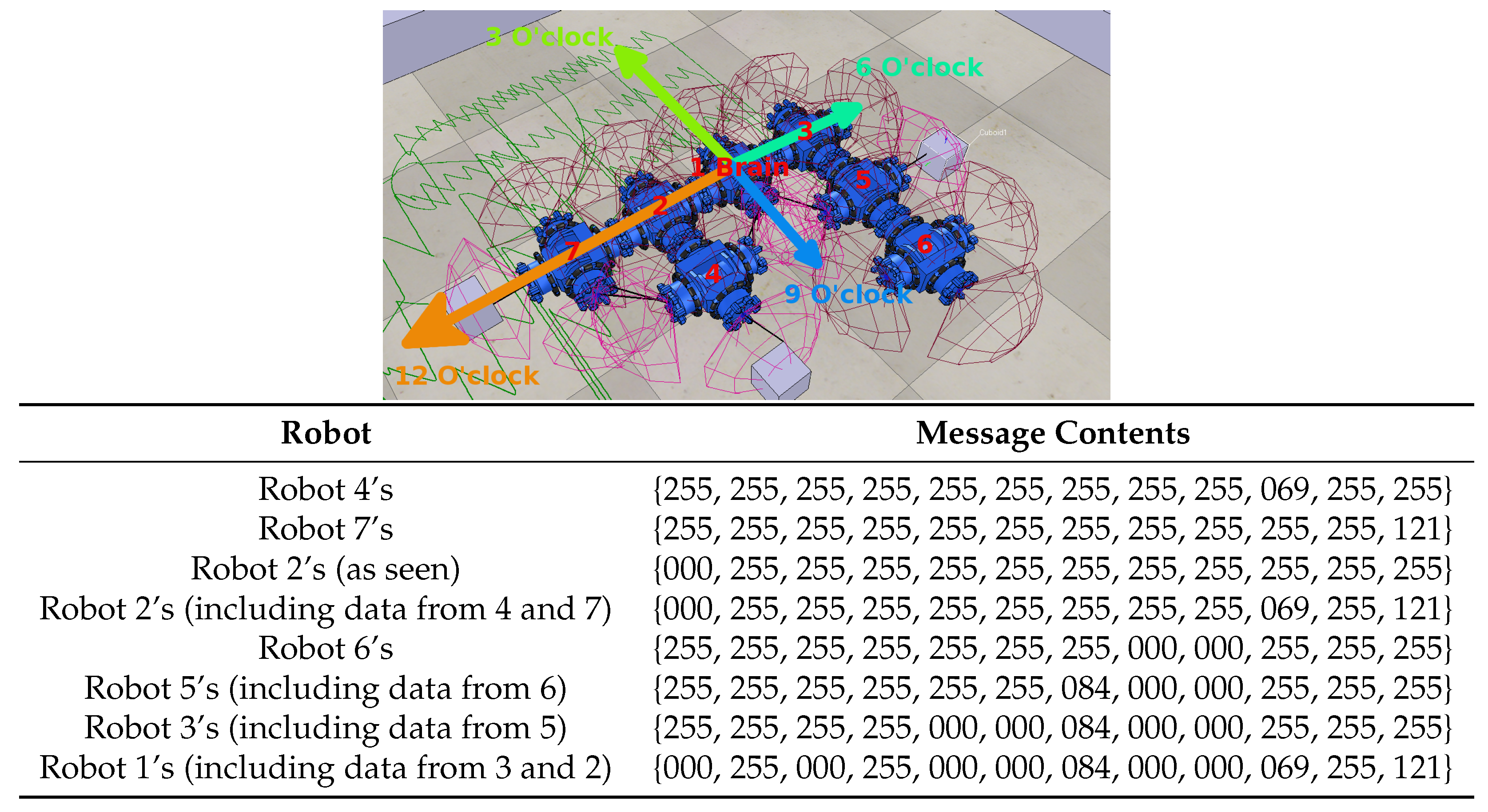
6.4. Mergeable Nervous Systems over Wi-Fi

If a failed module has slaves attached but none of these slaves have subslaves, then multiple single modules attached to different ports on the failed module must cooperate without having a direct physical connection. MNS actions can therefore be performed using Wi-Fi communication links in these circumstances. Temporary ID numbers, unique within an organism, are used to select which slave of the failed module will act as MNS master and which will become slaves to it. Unlike port-to-port IR communications, Wi-Fi communication also requires the permanent ID numbers of modules by which they will be addressed; modules, therefore, send broadcast Wi-Fi messages to all Wi-Fi addresses that act as requests for robots with the correct Temporary ID to respond with their Permanent ID. With this complete, MNS control can proceed ordinarily, except that the instantaneous centre of rotation calculation is modified to use the relative positions of modules separated by a failed module located inbetween them. The master of a Wi-Fi-controlled retreat substructure uses the same behaviours as an MRS module.

Once the failed module is discarded, the Wi-Fi controlled retreat structure breaks up into Lone Modules, each in the “Wandering” state. As this structure does not involve any connections between multiple operational robots, there is no point in attempting to recover it in the way that multi-robot substructures are re-recruited.

6.5. Recruiting a Replacement

We now consider the MFM module’s role throughout the self-repair process. Upon detaching from the failed module, it begins recruiting for a replacement module by entering the “Master of the Failed Module recruits for replacement” state. In this state, initial recruitment is identical to that used during self-assembly; however, once the recruited module, which will become the RM, has rotated to dock, an alternative form of recruitment is used at the time when the RM is in the “Approach to Dock” state.

Receipt of this specialised recruitment message type triggers the recruited robot to begin another new type of recruitment, Type 10, on its docking ports. Type-10 recruitment messages are emitted by the Replacement Module only on ports that require still existing multi-module structures to connect to them, and are readable only by MAS and MRS modules. The special roles performed by the MFM module cease to operate as soon as it is no longer recruiting on any ports; the RM module then takes over these tasks.

6.6. Guiding the Substructures

The features so far discussed are useful to dynamic self-repair, and many are newly implemented in the field of modular robotic self-repair, but it is the ability to operate while group motion is maintained that crucially distinguishes Dynamic Self-repair from earlier strategies.

Upon detaching from the failed module, the MFM begins transmitting a combination of wheel speed and compass data over Wi-Fi broadcast. These messages are read by the MAS and MRS modules and used to set reference frames from which their retreat and return motions are structured. Robots acting as MAS and MRS modules record the sum of the wheel speeds received over Wi-Fi and record the sums of their own motions to perform odometry calculations and calculate which driving direction will be necessary to return them to a region in which they will find the recruitment IR cone of the relevant docking port on the RM module.

Even in the idealised environment of simulation, this odometry data gives relatively poor readings, with returning modules often overshooting or undershooting the point at which they cross the trajectory of the main structure, hence missing the recruitment cones. Hence, the IR line of sight messaging is also used to guide MRS and MAS substructures back. The Replacement module within the main structure commands all undocked ports on the structure to, for a fraction of a second every few seconds, emit messages at full power. These messages identify which module, by Temporary ID, within the substructure is emitting the message. Any robot in an MAS- or MRS-controlled substructure may receive such messages and forward them on to the MRS of MAS module of its substructure. Using a combination of compass readings, for the emitting and receiving robots, and of Structure-Recruitment-List-derived knowledge of distances between robots with a given Temporary ID and the location of the RM within the main structure, an MRS or MAS robot can switch to a behaviour in which it attempts to enter the recruiting cone by “orbiting” around the main substructure in the direction, calculated from the Structure Recruitment List, that allows it to travel the shorter distance to reach the recruiting cone. Once within range, substructures manoeuvre under MNS control to dock to the RM and return the organism to its original form.

6.7. Dynamic Master Switching

A further version of the self-repair controller was created with additional features able to change the location of the master robot. Unlike the other strategies described, this one can replace a failed global master, exhibiting a form of neuroplasticity. In a Quadruplet list, each docked connection is specified in terms of which robot will be master within that connection, which will be the slave, and which port each will use. Whilst this Quadruplet array usually acts as a form of directed graph, it also contains all the information necessary to plot out alternative hierarchies of mastery able to represent the same structure. It is, therefore, possible to remap the location of the master within the organism, dynamically switching it between different robots while preserving connections and Temporary ID numbers.

Remapping occurs immediately after a failure is detected in a neighbouring module, and, as described with the earlier self-repair process, is handled independently by each module neighbouring the failed module, with the expectation that all will, as they have the same understanding of the structure and the failed module’s position within it, reach common conclusions on how to proceed with repair. The process takes a copy of the current Structure Recruitment List, which represents the structural plan regardless of the current physical state, and the Recruitment List, modified in real time to reflect docking and undocking events, and stores them in other variables. The Structure Recruitment List is then remapped to be centred, temporarily, on the failed robot. The Recruitment List is updated by remapping as necessary, to match the new Structure Recruitment List. With this temporary remapping in place, all other modules in the organism can be treated as slaves to the failed module, and sub-slave counting methods can compare the size of the structures connected to each of the failed module’s ports. Decisions can then be made on whether to transfer global mastery away from the current global master and in to part of the largest structure attached to the failed module, or revert to the copies taken of the unedited Quadruplet arrays. Such a transfer of global mastery is, of course, essential, if the global master is the failed module. A key point to note about the algorithms presented here is that, when used correctly, they cannot convert a physically feasible structure in to an impossible one during the process of remapping it.

After the remapping process is complete, modified Structure Recruitment Lists and Recruitment Lists are shared over Wi-Fi in a specialised “atomic” operation. This is necessary so that other modules within the organism, aside from those directly connected to the failed module that calculated the remapping for themselves, have the correct information necessary to supply mergeable nervous systems sensor data in the reference frame of their new master. An “atomic” operation is used to prevent the chaos that could ensue if modules received updates to the Structure Recruitment List and Recruitment List at different times and spent the intervening time with an updated copy of one but an obsolete copy of the other. As the remapping simply changes the order of terms inside specific Quadruplets within the Structure Recruitment List and Recruitment List arrays, no robot will have experienced any disruptive change, such as a modification of Temporary ID value, and no undocking or redocking is required for the master-switched structure to resume MNS activity.

As well as being able to recover from a failure of the global master, the Dynamic Master Switching strategy also provides an opportunity to allocate roles differently to the substructures around the failed module. Unlike with the earlier DSR strategy, if the largest group of modules connected to a failed module is a slave of the failed module, the largest substructure can be placed in charge of the re-recruitment part of self-repair and can contain the MFM module. Mergeable nervous systems over Wi-Fi methods can be prioritised where possible to allow the disposal of failed modules to be handled by single modules, which can be replaced individually, decreasing the need for large substructures to be guided back to dock after retreating and turning to dispose of a failed module. Where possible, if sufficient smaller substructures exist, larger substructures can be prioritised for MAS roles rather than MRS, meaning they will typically spend less time wandering away from the main structure and should be easier to guide back to dock once a Replacement Module is in place. However, if there are not sufficient individual modules connected to a failed module for a Wi-Fi-controlled retreat, and no smaller substructures available to act as MRS either, then the Dynamic Self-repair with Dynamic Master Switching strategy will allocate any available substructure to play the vital role of removing the failed module.

7. Self-Repair Experiments

Five forms of self-repair were compared. Dynamic Self-repair (DSR), Static Self-repair (SSR), naive Dynamic Self-repair (nDSR), naive Static Self-repair (nSSR) and Dynamic Self-repair with Dynamic Master Switching (DMS). Static Self-repair provides a close analogue to the strategies developed by Murray [10], acting like DSR but pausing the group motion at the moment of failure and remaining static until the structure is repaired. The two “naive” strategies are based on Murray’s full break-up strategy, which they labelled “naive”. The Omni-Pi-tent platform makes a complete breakup utterly superfluous, so in nDSR and nSSR a complete breakup is performed of everything below the failed module in the Recruitment List hierarchy, recursively transitioning all slaves and subslaves of the failed module into the “Wandering” state via “Escape Dock”, while leaving other sections of the structure unchanged. On the master side, naive self-repair involves only an undocking from the failed module and a brief retreat away from it so as to make space for replacements to be recruited; this re-recruitment is carried out exactly like ordinary self-assembly. In addition, nSSR and nDSR differ in that, in nDSR, Omni-Pi-tent’s ability to dock during motion means that the main structure can keep driving whilst this recruitment of a replacement and of replacement subslaves for it takes place.

Example videos of all five strategies are available in the Supplementary Material (S1–S5).

In the experiments performed to compare DMS, DSR, nDSR, SSR and nSSR self-repair strategies, a structure was initially formed at a starting point by self-assembly with the seed not moving. This initial self-assembly was necessary only because of the nature of the V-REP simulation and the difficulties V-REP would cause if one wished to initiate a simulation with modules already in a docked state; the time taken here did not count towards the measurements used in the analysis. Once self-assembly was complete, the structure began a drive towards the opposite end of a long arena, and the timer clock began. After starting motion, a failure was injected in to a selected module within the structure and the failed module’s port-to-port communication ceased. The task for the other modules in the structure was to identify this failure and self-repair, with static strategies stopping group motion to perform the repair and dynamic strategies continuing along the arena. The finishing time for each run was recorded as the moment when a completely repaired structure crossed a finishing line at the far end of the arena. In all scenarios, 30 robots were present in the scene at the start, an arena of 7 m width was used with the finish line placed 10 m away from the starting point, and 20 min of simulated time were given as a maximum time, after which a run was considered timed-out.

This scenario was run for seven different structures, see

Table 3. Structures used in the self-repair experiments, each structure is named with a Recruitment List and an image displayed. The seed robot (pink) and those that were injected with faults (yellow) are highlighted. Here, 10B, 12A and Rand are sourced from [10], the rest are derived from the self-assembly experiments, with S2 enlarged and modified to make the repair task more interesting.

Name	Image	Temp. IDs of Fault Injected Modules	Recruitment List
10B		5, 7	{{1,4,2,2},{1,3,3,3},{3,4,2,4}, {3,1,1,5},{5,4,2,6},{5,3,3,7}, {7,4,2,8},{7,1,1,9},{9,4,2,10}}
12A		2, 4	{{1,4,2,2},{1,1,4,6},{1,3,4,5}, {5,2,4,8},{6,2,4,7},{2,4,4,3}, {3,2,4,4},{4,1,4,11},{4,3,4,10}, {11,2,4,12},{10,2,4,9}}
Rand		6, 7, 9	{{1,2,2,2},{1,3,2,3},{1,4,2,4}, {4,4,3,5},{1,1,2,6},{6,4,2,7}, {7,1,4,8},{7,3,2,9},{9,4,3,10}, {10,1,1,11},{11,3,3,12}}
S1		2, 5	{{1,1,3,5},{1,3,1,2},{2,4,4,9}, {2,2,4,10},{2,3,2,3},{3,4,4,4}, {5,4,2,8},{5,1,2,6},{5,2,2,7}}
S2		4, 5	{{1,1,1,4},{1,2,2,2},{1,3,2,3}, {4,3,2,5},{5,3,2,6},{5,4,4,7}}
S3		2, 10	{{1,1,4,3},{1,2,4,10},{1,3,4,2}, {1,4,4,4},{4,2,2,5},{2,2,4,7}, {3,2,4,6},{7,3,3,8},{6,1,1,9}, {10,2,4,11},{11,1,2,12},{12,4,4,14}, {11,3,2,13},{13,4,4,15}}
S5		4, 7, 8	{{1,1,4,4},{1,3,4,7},{1,4,1,2}, {2,3,3,3},{4,3,4,5},{5,2,4,6}, {7,2,4,8},{8,3,3,9},{9,4,1,10}}

. For each structure, runs were performed involving the failure of a variety of different modules, as specified by Temporary ID number, within it. A total of 100 runs of each of the nSSR, SSR, nDSR DSR, and DMS strategies were performed for each combination of structure and failed robot.

Self-Repair Results

Table 4. Proportions of runs completed without timing out for the self-repair strategies under comparison. Yellow cells mark situations where, for a given structure and failed robot, a particular strategy achieved ≥ 60% success, green cells indicate completion rates ≥ 80%. Averages across all structures and failures tested give: nSSR 37%, nDSR 90%, SSR 72%, DSR 68% and DMS 76%. This indicates that both the motion involved in Dynamic strategies and the ability to self-repair both provide reliability advantages over static-self-assembly-based nSSR. SSR’s higher proportion of completed runs within the time limit suggests that DSR’s speed advantage is traded against a reduced reliability. As well as a higher averaged completion percentage than the standard DSR strategy, DSR with DMS managed a completion rate above 80% in 43% of scenarios to DSR’s 25%.

Structure	ID of Failed Module	nSSR	nDSR	SSR	DSR	DMS
10B	5	3%	95%	45%	72%	81%
10B	7	15%	99%	58%	72%	87%
12A	2	15%	79%	81%	62%	72%
12A	4	78%	99%	56%	61%	54%
Rand	6	15%	77%	69%	62%	52%
Rand	7	40%	71%	61%	62%	51%
Rand	9	12%	75%	62%	60%	64%
S1	2	53%	97%	63%	82%	94%
S1	5	45%	97%	99%	98%	97%
S2	4	61%	98%	98%	91%	82%
S2	5	67%	100%	99%	100%	99%
S3	2	3%	81%	32%	35%	68%
S3	10	5%	69%	60%	49%	69%
S5	4	90%	99%	91%	53%	78%
S5	7	18%	98%	74%	56%	81%
S5	8	68%	98%	99%	74%	85%

shows the proportions of repair operations that completed within the time limit, while

Table 5. A-test results showing effect sizes of the differences between distributions of total task-completion times. For each column of Strategy A vs. Strategy B, results show the chance that A will take longer than B. Green cells mark those for which the p-value indicated a statistically significant difference in strategy performance. In all statistically significant examples, nSSR is inferior, slower, than all other strategies. DSR and nDSR are often faster than SSR, with some exceptions where SSR outpaces nDSR. Furthermore, nDSR and DSR usually have similar performance, but where they are statistically significantly different, DSR proves faster. DSR with DMS proves statistically significantly different to nSSR in almost all scenarios, whilst differing from DSR and nDSR in fewer scenarios. DMS is faster than nDSR for a majority of scenarios and slower than standard DSR for more than half of the statistically different scenarios.

Structure	ID of Failed Module	nSSR vs. nDSR	nSSR vs. SSR	nSSR vs. DSR	nDSR vs. SSR	nDSR vs. DSR	SSR vs. DSR	nSSR vs. DMS	nDSR vs. DMS	SSR vs. DMS	DSR vs. DMS
10B	5	0.77	0.88	0.85	0.52	0.56	0.60	0.80	0.47	0.41	0.37
10B	7	0.88	0.89	0.90	0.31	0.45	0.60	0.82	0.34	0.50	0.40
12A	2	0.69	0.96	0.94	0.7	0.82	0.78	0.82	0.34	0.50	0.40
12A	4	0.84	0.81	0.89	0.29	0.52	0.80	0.83	0.47	0.74	0.45
Rand	6	0.67	0.94	0.98	0.72	0.89	0.90	0.89	0.79	0.74	0.49
Rand	7	0.55	0.75	0.74	0.57	0.58	0.62	0.70	0.58	0.59	0.51
Rand	9	0.82	0.92	0.91	0.57	0.67	0.68	0.91	0.67	0.73	0.49
S1	2	0.89	0.83	0.91	0.36	0.60	0.77	0.88	0.57	0.72	0.48
S1	5	0.93	0.79	0.93	0.16	0.45	0.84	0.95	0.47	0.89	0.52
S2	4	0.88	0.92	0.99	0.23	0.67	0.92	0.92	0.27	0.72	0.13
S2	5	0.95	0.86	0.95	0.13	0.52	0.87	0.95	0.74	0.91	0.67
S3	2	0.86	0.97	0.90	0.58	0.67	0.71	0.95	0.52	0.42	0.33
S3	10	0.65	0.95	0.96	0.71	0.85	0.85	0.93	0.85	0.85	0.52
S5	4	0.73	0.82	0.84	0.36	0.47	0.73	0.92	0.66	0.89	0.74
S5	7	0.91	0.96	0.94	0.42	0.55	0.70	0.94	0.66	0.83	0.64
S5	8	0.80	0.89	0.90	0.41	0.55	0.77	0.92	0.52	0.84	0.48

summarises the A-test scores when comparing task-completion times among the self-repair runs. Two example scenarios are shown with the graphs in Figure 12 and Figure 13.

The size of a structure below the failed module can be considered either as an absolute count of subslaves or as a measure of how large specific substructures below it are. Figure 14 shows task-completion times plotted against the number of robots below the failed robot in the hierarchy of a structure. Lines of best fit indicate how each strategy’s time-requirements scale with the number of robots below the failure site. Figure 15 explores the same trend but in terms of the largest single substructure below the failed module, rather than the total number of subslaves.

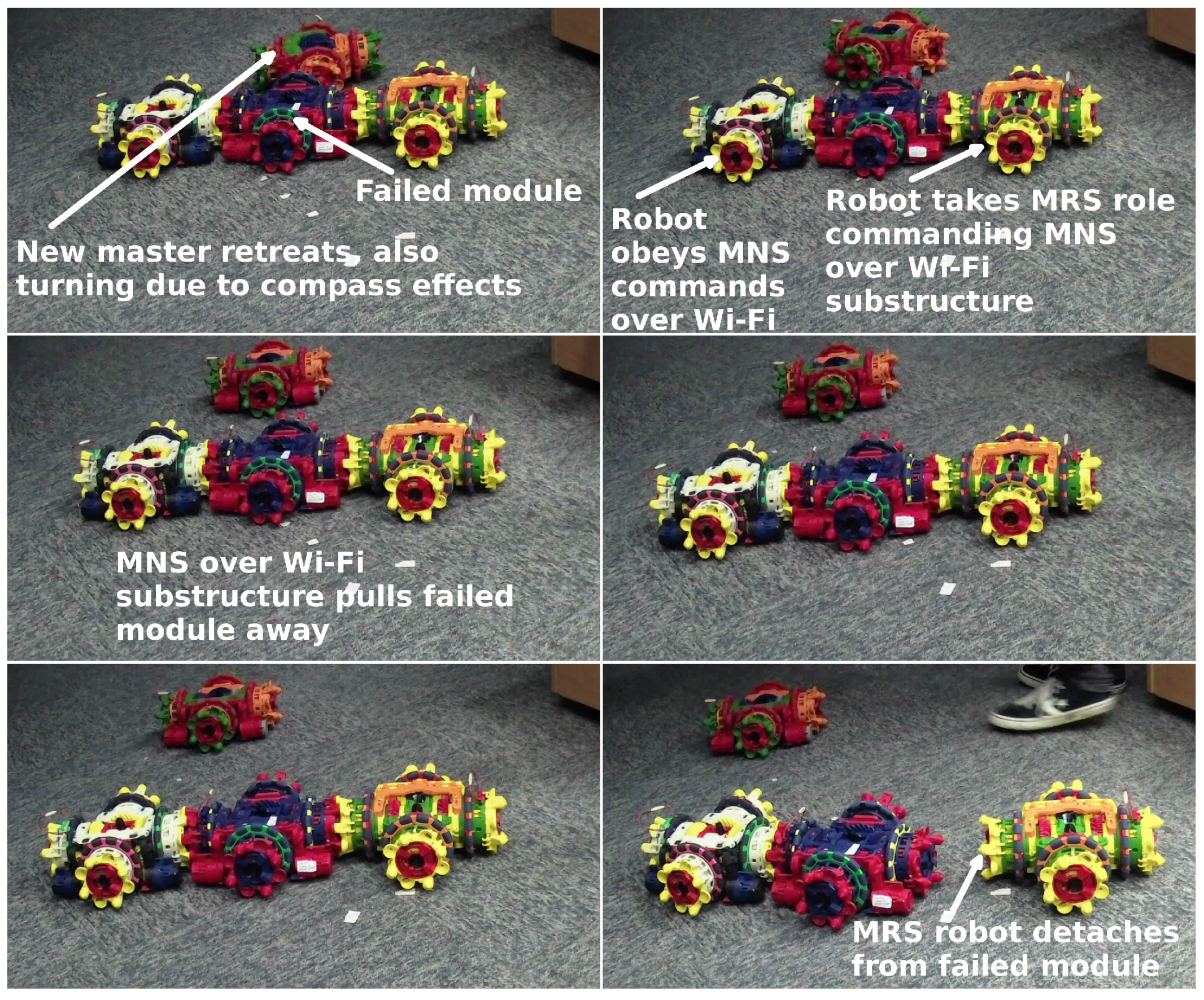
8. Hardware Demonstration of Principles

To demonstrate the feasibility of MLR self-assembly in hardware, robots were programmed with a C implementation of the MLR controller. It was known that the IR 38 KHz communications could prove unreliable, and features were added to the controller that broadcast copies of some of the IR message types over Wi-Fi, particularly the later parts of the recruitment handshaking procedure. The hardware implementation also added an extra state to the Finite State Machine, see Figure 2; this state, referred to as “Ramming Speed”, was placed between “Approach to Dock” and “In Organism”. This state was entered as soon as both docking switches on the appropriate port of a recruited robot were pressed, indicating reaching the docking position, and lasted for 3 s, during which the recruited robot drives at full speed against the port to maintain good contact while its hooks lock (a 0.3 s procedure), after which the robot transitions to the “In Organism” state and acts equivalently to in simulation. This is in contrast to simulations where docking actuation is instant.

A robot within the swarm was manually instructed to become seed for one of two different structures, a T-shaped structure ({{1,1,1,2},{1,3,1,3},{1,4,1,4}}) or an S-shaped structure ({{1,2,2,2},{2,3,4,3},{3,3,1,4}}), and began moving along a northward direction calculated from its compass readings. Due to the limited number of robots available, it was not feasible for random wandering to bring robots within recruitment range regularly; hence, other modules were placed in regions where they could receive its recruitment communications over IR and be allowed to dock autonomously from there. Robots were allowed to dock to form the structures and navigated themselves for both positioning and compass alignment; some of the placed robots were put at 90° or 180° away from the orientations but, nonetheless, still aligned and docked. Figure 16A shows an example of these docking operations. Further robots docked until the structure was formed. The multi-robot structures were then allowed to move around and avoid obstacles to provide proof of the MNS capabilities. Videos of some of these recruitment events and of coordinated group motion are provided in the Supplementary Materials (S6).

During docking it was found that real world non-uniformity in magnetic fields meant that, in the distance between two connected robots, the field often turned by up to 10°, so robots coming together would often be 10° off compass alignment. Random noise of $\pm 5$°, varying every 0.6 s, was added to the compass reading during final approach for docking, ensuring that, sooner or later, the two modules would align their hooks to within the angle accuracy needed to dock successfully. This magnetic field non-uniformity did not affect robots once docked within an organism, as our MNS implementation was carefully designed to avoid explicit reference to local compass readings and handle all data in the reference frame of the master robot with inter-robot angles calculated by knowledge of port-to-port links and not by compass readings.

A notable problem encountered was establishing whether a robot was docked on any given port. Whilst a simple check to perform in simulation, the physical hardware’s tolerances are such that, when two robots are docked, there is sufficient play within the mechanism to allow for the contact switches to break contact even whilst a dock exists. When determining whether a port is docked, there are two considerations of importance, the first is simple, knowing whether a robot’s own docking hooks on a particular port are locked or unlocked; the second is knowing whether the other robot involved in the dock is present and has its hooks locked. Methods based on low pass filtering the docking switch states to remove brief fluctuations struggled to tell the repeated impacts on each switch involved in pre-docking manoeuvres from a successful dock, and also incorrectly assumed a dock no longer existed when robots were driving in such a direction as to relieve the pressure on the switches for significant time periods. Wi-Fi communications were used to let robots agree that a dock had formed between them, with any robot undocking sending a Wi-Fi message to this effect. However, reliance on communications to signal the making and breaking of docked connections allowed for occasional incidents where a robot wrongly believed itself to be docked, and was believed by its immediate master to have docked, despite having become disconnected in the 0.3 s between beginning actuating the docking hooks and having them reach the locked position due to the master robot moving at that instant in ways that “Ramming Speed” was not able to correct for. Almost all activities with modular robots would appear to require reliable ways for a robot to check at any given moment whether any given one of its ports is docked, so it may not be possible to develop controllers that can achieve desirable levels of reliability without accurate “dock-presence sensing”.

Difficulties were also encountered in some runs due to the replacement of line-of-sight IR communications in some roles with universally available Wi-Fi messages. This made the non-conflict docking procedures more difficult, as only the initial recruitment messages were now sent over the line-of-sight IR system. With short-range verification messaging not able to work reliably, this too had to be replaced with Wi-Fi; therefore, in a small number of cases robots were able to dock to ports other than the one that they thought they were approaching. Unable to rely on the readings of the contact switches, robots were not able to easily detect such incorrect dockings. Further Wi-Fi handshaking could not entirely mitigate this, as they were not position-dependent in the way that the IR was designed to be. These problems show the benefit that line-of-sight communication can bring if it is reliable, particularly that approximate positional information can be inferred and that receipt of certain message types guarantees relative positions, and the hazards of trying to work around line-of-sight to use global communications. It is worth repeating that the difficulties caused by a lack of line-of-sight communication here show that line-of-sight communication is not inferior to global communication in all modular robotics applications, despite the popularity of broadcast methods [49].

The mergeable nervous systems-inspired [41] co-ordinated group-control methods worked extremely well, giving reliable control of the multi-robot organism. Tests were performed by placing an IR-reflecting obstacle into various positions around a completed, or partially completed, organism and watching its reactions. Obstacles placed beside any docking port, whether on the seed robot, on a robot connected to the seed, or on a robot two layers away from the seed, were detected and the structure retreated away from them according to the clock direction in which they were observed. Ports facing towards other parts of the structure were, as intended, not sensitive to obstacles. Rotation of the robotic group was also demonstrated.

Out of 26 dockings attempted between wandering modules and moving recruiters, 20 of these actions succeeded; those which failed were mostly due to the approaching robot timing out of the docking attempt after taking too long.

Tests were also performed to demonstrate MLR’s use of co-ordinated docking between robotic groups. For the S-shaped structure, a robot entering the position equivalent to a Temporary ID of 3 was allowed to complete the handshaking procedure and then temporarily manually restrained. An extra robot was placed close by this robot’s Port 3 and allowed to dock to it. The robot with a Temporary ID of 3 was then released, to act as master of a two robot group and attempt docking to the seed robot. Figure 16B shows this. It was difficult to create the circumstances for this event and the robot with a Temporary ID of 3 usually completed a docking to the seed before its subslave could be introduced to the area. This proves the principle of MLR to be feasible with hardware, and matches up with the simulations, which show a lack of significant difference between MLR and LW + MNS performance, in that most of the time robots did not typically form such substructures before docking, due to speed considerations involved.

Self-Repair and the Reality Gap

For self-repair demonstrations, modules were manually placed for quick initial self-assembly; then, once they were moving, a switch was pressed on one module to trigger a failure mode. In this failure mode, the module’s wheels stopped, all IR and Wi-Fi communications ceased, and proximity sensing was disabled. Connected modules were required to detect the failure, then remap their structure and take on appropriate roles for self-repairing. Once the failed module had been removed, it was manually released from its failure mode and the software reinitialised such that it acted as a free wandering robot. The limited number of modules available meant that providing a spare module to become the Replacement module would too-greatly limit the structure sizes possible, so the failure mode was made reversible, with the failed module transitioning to “Wandering” after being dumped. It was then allowed to dock again either as the Replacement Module or as a recruit to replace other parts of the broken-up structure when mergeable nervous systems over Wi-Fi was in use.

With only four hardware modules available, scenarios involving large substructures could not be created, a T structure was used with a failure induced in the global master. After Dynamic Master Switching processes had occurred, see the Supplementary Material for video footage (S7), mergeable nervous systems over Wi-Fi was automatically selected by the robots as the method for removing the failed module. Unfortunately, the two modules available to remove the failed module had insufficient torque to drag it when its wheels were stationary. The controller was modified to allow a failed module to still listen to MNS-actuation commands over Wi-Fi from the robot commanding its removal; however, these communications were not always acted upon correctly by the failed robot, likely due to other effects created by the failure state induced. Figure 17 shows the attempt in progress; the failed module followed the Wi-Fi commands at some points but at others the whole retreating structure was stalled when it did not. The master-side section of the robotic organism did, nonetheless, successfully escape and begin re-recruitment.

This demonstration showed the ability of modules to detect a failed neighbour, and showed Dynamic Master Switching working over Wi-Fi. Although coding errors made it difficult to return a module to correct operation after a failure was induced, one incident was observed in which modules that had attempted an MNS over Wi-Fi retreat were re-recruited to partially rebuild the structure; see the Supplementary Material (S7).

Another demonstration was attempted where Dynamic Master Switching features were disabled to allow ordinary Dynamic Self-repair to occur; this was intended to cause a situation where the docking of a multi-module substructure to the newly recruited Replacement module could be observed. An S structure was used with the fault injected such that a two-module MRS substructure was formed. This demonstration, however, suffered from a number of reality-gap issues. The difficulties inherent in dock detection meant robots struggled to recognise undocking events, Recruitment Lists shared between them were therefore often inaccurate descriptions of the structure’s current state. Compared to self-assembly, the requirements that self-repair places upon the reliability of docking detection equipment are far more exacting. Whilst in self-assembly the difficulties could be overcome with software work-arounds, self-repair’s more frequent and repetitive docking and undocking events overwhelmed the ability of software work-arounds to accurately keep track of the port states. This provides an example of how self-repair proves to be a much more complex task than self-assembly, not only at the theoretical level and in the design of robotic controller software, but also at the practical level in ways that do not become apparent until real hardware is involved.

As successful removal of a failed module could not be performed, it was not feasible to test in hardware the guidance methods to return substructures to the main organism. However, by providing proof that it is possible for neighbouring hardware modules to detect failed modules, and given that the mergeable nervous systems and Multi-Layered Recruitment hardware demonstrations showed that the collaborative driving necessary for removing failed modules and for returning substructures to dock is possible, achieving Dynamic Self-repair with hardware would appear to be primarily a matter of improving wheel torques, docking detection and line-of-sight communication reliability.

9. Discussion

9.1. Self-Assembly

In the scenarios where a low p-value shows a strong statistical difference between strategy performance, the dynamic self-assembly strategies produce A-test measures indicating their superiority; in many of these scenarios dynamic self-assembly methods perform better in over 90% of randomised runs. The LW + MNS and MLR scenarios rarely see a statistically significant performance difference.

Significantly low p-values (<0.05) from the comparison, for most scenarios, of the LW+ distribution to the LW + MNS or MLR distributions allow a null hypothesis that being able to assemble in motion has no effect on task-completion times to be rejected. Effect sizes for the comparison of these strategies all favour the self-assembly strategies that can assemble during motion; for many of the scenarios these effect sizes are extremely strong indeed.

MLR and LW + MNS do not substantially differ in performance; this may be due to the existence of a maximum possible wheel speed for robots. A robot undergoing recruitment, therefore, in the “Rotate to Dock” or “Approach to Dock” phase of the finite state machine, must move so as to match the motions of the recruiter’s reference frame and travel towards the recruiting port. It would appear sensible to use, once speed matching to the recruiter is achieved, whatever reserves of possible motor speed are left to perform this approach. Robots, therefore, attempt this approach at somewhere at, or above, 70% of their maximum wheel speed. Any robot recruited to a moving module will have only up to 30% of wheel speed with which to approach towards it. MLR therefore often does not, in practice, result in multi-module structures forming around a robot, as it is still in its “Approach to Dock” state. The only way that such formation would become more common would be if robots used lower speeds for their approach to recruiting ports. It appears unlikely that slowing the speeds, as a percentage of the maximum wheel speed, used for the approach would hasten assembly overall and it would make timing-out, entering the “Escape Dock” state, more common. Optimising the wheel speeds used during docking to see whether it is more beneficial to overall self-assembly time to use a slow approach, with more scope for multiple layers of recruitment, or a fast approach, despite the reduction in opportunities for multi-layered recruitment that this would cause, could be an interesting topic for further research. It is perhaps, therefore, best considered that while MLR provides an interesting idea, and a useful stepping-stone from which further capabilities could be built, it is not in itself able to, typically, provide significantly better performance, when self-assembling while in motion, than the LW + MNS strategy.

While the simulated experiments showed the performance benefits of self-assembly during motion, hardware experiments proved its practical feasibility, with docking to a moving target and coordinated MNS control of a structure shown to be reliable, once workarounds had been implemented to account for communication and sensing limitations, in the real world. This is the first demonstration of self-assembly during motion with modular robots. It is also of interest to note that the improved co-ordination of modules demonstrated here may, in future, allow simulated work that requires complex robot navigation [27] to become feasible to physically implement.

9.2. Self-Repair

Comparison of the proportion of runs that completed without timing out gives an indication of the reliability of a particular self-repair strategy. Indeed, nDSR’s high proportion of successful runs across all scenarios indicates reliability. The two substructure-based self-repair strategies displayed levels of reliability that varied across scenarios. Indeed, nSSR performed very poorly in this regard; nDSR and DSR both have greater chances of encountering wandering modules to recruit as replacements than static strategies, with the main limitation of DSR being the difficulty of guiding the removal-handling substructure back to dock. The main lesson here appears to be that for industrially useful self-repair, with a near 100% completion rate within some timeframes, more work must be carried out on extending the range of guidance and finding solutions to aid in navigation over distance; when subject to the condition of not relying on explicit GPS-style location data, this is an interesting problem for sensor-development and search-pattern driving algorithms.

The ability to repair while in motion, both for nDSR and DSR, gave statistically significant performance differences, with p-values below the 5% threshold in most scenarios. A-test results largely above 0.8 in statistically significant scenarios show nDSR outperformed nSSR, and A-test results above 0.7 for a vast majority of scenarios also show DSR’s speed advantage over SSR. A null hypothesis that being able to repair during motion has no effect on task-completion times can be confidently rejected; dynamic strategies regularly outperform their equivalent static strategies. Performing both the repair and motion tasks in parallel rather than serial can be considered as one of the causes behind this effect. This provides a good indication of the assistance that Dynamic Self-repair methods can provide for scenarios where overall task time is the key measurement, such as for reducing accumulated radiation doses.

The advantage provided by strategies able to operate in motion does little to accelerate the repair procedure itself, despite the speed advantages which it provides for the overall task being attempted. Whilst DSR and nDSR mostly outperformed nSSR, the SSR strategy proved most effective in terms of time for the repair itself to complete. Differences, measured in seconds, between different strategies’ times to perform the repair operation itself tend to be considerably smaller than the differences in task-completion times, showing that the differences in repair times are not the main cause for the differences in task-completion times. The repair procedure itself is observed to be significantly faster when substructure rather than breakup strategies are in use.

Naive-breakup-based strategies were outperformed in terms of task-completion times by substructure-based self-repair in some of the scenarios. Across static strategies, SSR performed faster than nSSR by a statistically significant amount for all combinations of structure and failed module; A-test scores for the effect size were all high, with many above 0.90. This provides a replication of some of Murray’s findings [10] with a new platform and code base. When comparing between dynamic strategies, the situation is less clear, with statistically significant differences only occurring in 7 of the 16 scenarios. In those scenarios where statistically significant differences were found, all favoured the substructure-based DSR over the breakup-based nDSR, with A-test scores ranging from 0.6 to 0.89. It is possible here that the extremely high reliability of nDSR makes it difficult for DSR, a less-reliable strategy, to substantially outperform it in many of the statistically similar scenarios; improving sensors or search patterns may change this. DSR may also display a lesser advantage over nDSR than SSR does over nSSR due to the increased probability of substructures involved in the repair getting lost whilst attempting to relocate the main structure, a scenario less likely to happen when the main structure remains static.

The experiments found, for SSR and DSR, no strong evidence of correlations between either the total number of subslaves below a failed module in a hierarchy, or the number of modules in the largest single substructure formed during self-repair by the failed module’s slaves. Both static and dynamic self-repair methods allow for task-completion times that do not appear to scale up with structure size by either the subslave count or largest substructure measure. Task-completion times do, however, rise, with Pearson correlation coefficients in the range of 0.18 to 0.40 for breakup-based strategies. Furthermore, nDSR has the strongest correlation coefficient, being strongest when compared against the size of the largest substructure rather than the total subslave count. This suggests that naive-breakup-based strategies are less scalable than substructure preserving self-repair; that the size of the largest substructure has a stronger effect than the total subslave count also indicates that an increased number of “layers” on which the re-assembly must take place may be of importance here. Breakup-based strategies lose performance, relative to substructure-preserving ones, as the number of modules and size of substructures below the repair site rises. The relative performance of DSR against SSR stays constant with structure sizing, showing that the beneficial effect of being able to self-repair during motion remains roughly constant with structure size.

The DMS strategy largely performs similarly to DSR, with, overall, no statistically significant speed benefit above DSR. However, the ability to switch master location enables repairs in scenarios that the other strategies cannot handle, such as the failure of the global master, and provides reliability improvements due to the use of smaller removal substructures and therefore reduced opportunities for substructures to become lost while guiding themselves back to dock.

Hardware demonstrations found self-repair to be a much more difficult task than self-assembly, with sensor, communication and wheel torque limitations proving particularly problematic. The practicality of detecting a module failure via a lack of port-to-port communications from it was verified, and the ability of the master side neighbour of a failed module to retreat was shown. Dynamic master switching was demonstrated to work on real robots with Recruitment Lists correctly updated and transferred. The feasibility of the underlying principles for dynamic self-repair has therefore been demonstrated, but fully proving its practicality was not possible with this hardware. The importance of implicit information in communications is highlighted by the difficulties encountered. Such difficulties encountered also suggest that successful completion of dynamic self-repair strategies may be a worthwhile benchmarking test to compare the performance of modular robotic platforms.

10. Conclusions

This paper has proposed and demonstrated new strategies for self-assembly and self-repair with modular robots during motion. It has been explained how the unique features of the Omni-Pi-tent platform make such strategies feasible and discussion of implementation details has been presented. The new self-assembly strategies were compared against a “classical” self-assembly to a static seed, inspired by Liu and Winfield’s work. It was found that, in all scenarios for which conclusive data could be gathered, one or both dynamic self-assembly strategies had statistically significantly better performances. Hardware tests verified the feasibility of docking and mergeable nervous systems group control, and showed self-assembly during motion as well as multi-layered scenarios. No prior self-assembly work has managed to operate at all with co-ordinated group motion occurring while assembly progresses. The new self-repair strategies were compared against methods inspired by Murray’s work, strategies able to repair during motion were found to lead to faster task completion than strategies requiring motion to halt for repair to be undertaken; strategies able to use substructures were found to be faster to complete and more scalable than strategies requiring the breakup of structures. Hardware demonstrations proved many of the fundamental activities required for dynamic self-repair, but could not achieve the full procedure due to reality-gap issues. The challenges encountered indicate the exacting demands self-repair places on hardware and connector interface reliability, above those required to allow self-assembly.

Future work could focus on modifying self-assembly and self-repair methods to handle loops, potentially by forming multiple non-loop-containing structures then bringing them together under MNS control, and rules regarding specialised heterogeneous modules within an organism, as well as 3-dimensional self-assembly and self-repair via the use of module hinge joints and improved long-range robot guidance methods and post-disassembly search patterns to aid in relocating modules during self-repair. Such search patterns may be able to draw inspiration from those used at sea to locate drifting objects. There are also possibilities for performing self-repair where detached sections of the structure may re-assemble to replace parts of a morphology that are not the same sections which they previously acted as, potentially adapating some of [26]’s findings for use in this context. Due to the hardware findings of the importance of reliable docking, dock detection, and port-to-port communication equipment for modular robots, another major aspect of future work would be refining those systems and developing standards for use in future modular robotic designs.

References

1. Fukuda, T.; Nakagawa, S. Dynamically reconfigurable robotic system. In Proceedings of the 1988 IEEE International Conference on Robotics and Automation, Philadelphia, PA, USA, 24–29 April 1988; pp. 1581–1586. [Google Scholar] [CrossRef]
2. Yim, M.; Shen, W.M.; Salemi, B.; Rus, D.; Moll, M.; Lipson, H.; Klavins, E.; Chirikjian, G.S. Modular self-reconfigurable robot systems [grand challenges of robotics]. IEEE Robot. Autom. Mag. 2007, 14, 43–52. [Google Scholar] [CrossRef]
3. Levi, P.; Kernbach, S. Symbiotic Multi-Robot Organisms: Reliability, Adaptability, Evolution; Springer Science & Business Media: Berlin/Heidelberg, Germany, 2010; Volume 7. [Google Scholar] [CrossRef]
4. Davey, J.; Kwok, N.; Yim, M. Emulating self-reconfigurable robots-design of the SMORES system. In Proceedings of the 2012 IEEE/RSJ International Conference on Intelligent Robots and Systems, Algarve, Portugal, 7–12 October 2012; pp. 4464–4469. [Google Scholar] [CrossRef]
5. Kernbach, S.; Meister, E.; Scholz, O.; Humza, R.; Liedke, J.; Ricotti, L.; Jemai, J.; Havlik, J.; Liu, W. Evolutionary robotics: The next-generation-platform for on-line and on-board artificial evolution. In Proceedings of the 2009 IEEE Congress on Evolutionary Computation, Trondheim, Norway, 18–21 May 2009; pp. 1079–1086. [Google Scholar] [CrossRef] [Green Version]
6. Parrott, C.; Dodd, T.J.; Groß, R. HyMod: A 3-DOF hybrid mobile and self-reconfigurable modular robot and its extensions. In Distributed Autonomous Robotic Systems; Springer: Berlin/Heidelberg, Germany, 2018; pp. 401–414. [Google Scholar] [CrossRef]
7. Peck, R.H.; Timmis, J.; Tyrrell, A.M. Omni-pi-tent: An omnidirectional modular robot with genderless docking. In Proceedings of the Annual Conference Towards Autonomous Robotic Systems, London, UK, 3–5 July 2019; Springer: Cham, Switzerland, 2019; pp. 307–318. [Google Scholar] [CrossRef]
8. Hancher, M.D.; Hornby, G.S. A modular robotic system with applications to space exploration. In Proceedings of the 2nd IEEE International Conference on Space Mission Challenges for Information Technology (SMC-IT’06), Pasadena, CA, USA, 17–20 July 2006; pp. 1–8. [Google Scholar] [CrossRef]
9. Baca, J.; Hossain, S.; Dasgupta, P.; Nelson, C.A.; Dutta, A. Modred: Hardware design and reconfiguration planning for a high dexterity modular self-reconfigurable robot for extra-terrestrial exploration. Robot. Auton. Syst. 2014, 62, 1002–1015. [Google Scholar] [CrossRef]
10. Murray, L. Fault Tolerant Morphogenesis in Self-Reconfigurable Modular Robotic Systems. Ph.D. Thesis, University of York, York, UK, 2013. [Google Scholar]
11. Jahanshahi, M.R.; Shen, W.M.; Mondal, T.G.; Abdelbarr, M.; Masri, S.F.; Qidwai, U.A. Reconfigurable swarm robots for structural health monitoring: A brief review. Int. J. Intell. Robot. Appl. 2017, 1, 287–305. [Google Scholar] [CrossRef] [Green Version]
12. Peck, R.H.; Timmis, J.; Tyrrell, A.M. Towards Self-repair with Modular Robots During Continuous Motion. In Proceedings of the Towards Autonomous Robotic Systems: 19th Annual Conference, TAROS 2018, Bristol, UK, 25–27 July 2018; Springer: Berlin/Heidelberg, Germany, 2018; Volume 10965, pp. 457–458. [Google Scholar]
13. Liu, W.; Winfield, A.F. Autonomous morphogenesis in self-assembling robots using IR-based sensing and local communications. In Proceedings of the International Conference on Swarm Intelligence, Brussels, Belgium, 8–10 September 2010; Springer: Berlin/Heidelberg, Germany, 2010; pp. 107–118. [Google Scholar] [CrossRef] [Green Version]
14. Tomita, K.; Murata, S.; Kurokawa, H.; Yoshida, E.; Kokaji, S. Self-assembly and self-repair method for a distributed mechanical system. IEEE Trans. Robot. Autom. 1999, 15, 1035–1045. [Google Scholar] [CrossRef]
15. Rohmer, E.; Singh, S.P.; Freese, M. V-REP: A versatile and scalable robot simulation framework. In Proceedings of the 2013 IEEE/RSJ International Conference on Intelligent Robots and Systems, Tokyo, Japan, 3–7 November 2013; pp. 1321–1326. [Google Scholar] [CrossRef]
16. Groß, R.; Dorigo, M. Self-assembly at the macroscopic scale. Proc. IEEE 2008, 96, 1490–1508. [Google Scholar] [CrossRef] [Green Version]
17. Rus, D.L.; Gilpin, K.W. Modular robot systems. IEEE Robot. Autom. Mag. 2010, 17, 38–55. [Google Scholar] [CrossRef]
18. Tucci, T.K.; Piranda, B.; Bourgeois, J. A distributed self-assembly planning algorithm for modular robots. In Proceedings of the International Conference on Autonomous Agents and Multiagent Systems, Stockholm, Sweden, 10–15 July 2018. [Google Scholar] [CrossRef]
19. Bererton, C.; Khosla, P.K. Towards a team of robots with repair capabilities: A visual docking system. In Experimental Robotics VII; Springer: Berlin/Heidelberg, Germany, 2001; pp. 333–342. [Google Scholar] [CrossRef] [Green Version]
20. Rubenstein, M.; Payne, K.; Will, P.; Shen, W.M. Docking among independent and autonomous CONRO self-reconfigurable robots. In Proceedings of the IEEE International Conference on Robotics and Automation, New Orleans, LA, USA, 26 April–1 May 2004; ICRA’04. Volume 3, pp. 2877–2882. [Google Scholar] [CrossRef] [Green Version]
21. Rubenstein, M.; Cornejo, A.; Nagpal, R. Programmable self-assembly in a thousand-robot swarm. Science 2014, 345, 795–799. [Google Scholar] [CrossRef] [PubMed]
22. Doursat, R. Organically grown architectures: Creating decentralized, autonomous systems by embryomorphic engineering. In Organic Computing; Springer: Berlin/Heidelberg, Germany, 2009; pp. 167–199. [Google Scholar] [CrossRef] [Green Version]
23. Nagpal, R. Programmable Self-Assembly: Constructing Global Shape Using Biologically-Inspired Local Interactions and Origami Mathematics. Ph.D. Thesis, Massachusetts Institute of Technology, Cambridge, MA, USA, 2001. [Google Scholar]
24. Werfel, J. Biologically realistic primitives for engineered morphogenesis. In Proceedings of the International Conference on Swarm Intelligence, Beijing, China, 12–15 June 2010; Springer: Berlin/Heidelberg, Germany, 2010; pp. 131–142. [Google Scholar] [CrossRef]
25. Stoy, K. Using cellular automata and gradients to control self-reconfiguration. Robot. Auton. Syst. 2006, 54, 135–141. [Google Scholar] [CrossRef]
26. Dutta, A.; Dasgupta, P.; Nelson, C. Distributed configuration formation with modular robots using (sub) graph isomorphism-based approach. Auton. Robots 2019, 43, 837–857. [Google Scholar] [CrossRef] [Green Version]
27. Li, H.; Wang, T.; Chirikjian, G.S. Self-assembly Planning of a Shape by Regular Modular Robots. Adv. Reconfig. Mech. Robot. II 2016, 36, 867–877. [Google Scholar] [CrossRef]
28. Yim, M.; Shirmohammadi, B.; Sastra, J.; Park, M.; Dugan, M.; Taylor, C.J. Towards robotic self-reassembly after explosion. In Proceedings of the 2007 IEEE/RSJ International Conference on Intelligent Robots and Systems, San Diego, CA, USA, 29 October–2 November 2007; pp. 2767–2772. [Google Scholar] [CrossRef] [Green Version]
29. Christensen, A.L.; O’Grady, R.; Dorigo, M. SWARMORPH-script: A language for arbitrary morphology generation in self-assembling robots. Swarm Intell. 2008, 2, 143–165. [Google Scholar] [CrossRef]
30. Baca, J.; Yerpes, A.; Ferre, M.; Escalera, J.A.; Aracil, R. Modelling of modular robot configurations using graph theory. In Proceedings of the International Workshop on Hybrid Artificial Intelligence Systems, Burgos, Spain, 24–26 September 2008; Springer: Berlin/Heidelberg, Germany, 2008; pp. 649–656. [Google Scholar] [CrossRef] [Green Version]
31. Liu, C.; Lin, Q.; Kim, H.; Yim, M. SMORES-EP, a Modular Robot with Parallel Self-assembly. arXiv 2021, arXiv:2104.00800. [Google Scholar]
32. Wei, H.; Li, D.; Tan, J.; Wang, T. The distributed control and experiments of directional self-assembly for modular swarm robots. In Proceedings of the 2010 IEEE/RSJ International Conference on Intelligent Robots and Systems, Taipei, Taiwan, 18–22 October 2010; pp. 4169–4174. [Google Scholar] [CrossRef]
33. Murata, S.; Yoshida, E.; Kurokawa, H.; Tomita, K.; Kokaji, S. Self-repairing mechanical systems. Auton. Robots 2001, 10, 7–21. [Google Scholar] [CrossRef]
34. Fitch, R.; Rus, D.; Vona, M. A basis for self-repair robots using self-reconfiguring crystal modules. In Proceedings of the Intelligent Autonomous Systems, Singapore, 22–25 June 2000; Volume 6, pp. 903–910. [Google Scholar]
35. Ackerman, M.K.; Chirikjian, G.S. Hex-DMR: A modular robotic test-bed for demonstrating team repair. In Proceedings of the 2012 IEEE International Conference on Robotics and Automation, St Paul, MN, USA, 14–18 May 2012; pp. 4148–4153. [Google Scholar] [CrossRef]
36. O’Grady, R.; Pinciroli, C.; Groß, R.; Christensen, A.L.; Mondada, F.; Bonani, M.; Dorigo, M. Swarm-bots to the rescue. In Proceedings of the European Conference on Artificial Life, Budapest, Hungary, 13–16 September 2009; Springer: Berlin/Heidelberg, Germany, 2009; pp. 165–172. [Google Scholar] [CrossRef] [Green Version]
37. Arbuckle, D.; Requicha, A.A. Self-assembly and self-repair of arbitrary shapes by a swarm of reactive robots: Algorithms and simulations. Auton. Robots 2010, 28, 197–211. [Google Scholar] [CrossRef]
38. Stoy, K.; Nagpal, R. Self-repair through scale independent self-reconfiguration. In Proceedings of the 2004 IEEE/RSJ International Conference on Intelligent Robots and Systems (IROS) (IEEE Cat. No. 04CH37566), Sendai, Japan, 28 September–2 October 2004; Volume 2, pp. 2062–2067. [Google Scholar] [CrossRef]
39. Rubenstein, M.; Shen, W.M. Scalable self-assembly and self-repair in a collective of robots. In Proceedings of the 2009 IEEE/RSJ International Conference on Intelligent Robots and Systems, St. Louis, MO, USA, 10–15 October 2009; pp. 1484–1489. [Google Scholar] [CrossRef] [Green Version]
40. Christensen, D.J. Experiments on fault-tolerant self-reconfiguration and emergent self-repair. In Proceedings of the 2007 IEEE Symposium on Artificial Life, Honolulu, HI, USA, 1–5 April 2007; pp. 355–361. [Google Scholar] [CrossRef] [Green Version]
41. Mathews, N.; Christensen, A.L.; O’Grady, R.; Mondada, F.; Dorigo, M. Mergeable nervous systems for robots. Nat. Commun. 2017, 8, 439. [Google Scholar] [CrossRef] [PubMed] [Green Version]
42. Zhang, Y.; Song, G.; Liu, S.; Qiao, G.; Zhang, J.; Sun, H. A modular self-reconfigurable robot with enhanced locomotion performances: Design, modeling, simulations, and experiments. J. Intell. Robot. Syst. 2016, 81, 377–393. [Google Scholar] [CrossRef]
43. Popesku, S.; Meister, E.; Schlachter, F.; Levi, P. Active wheel-An autonomous modular robot. In Proceedings of the 2013 6th IEEE Conference on Robotics, Automation and Mechatronics (RAM), Manila, Philippines, 12–15 November 2013; pp. 97–102. [Google Scholar] [CrossRef]
44. Jakobi, N.; Husbands, P.; Harvey, I. Noise and the reality gap: The use of simulation in evolutionary robotics. In Proceedings of the European Conference on Artificial Life, Granada, Spain, 4–6 June 1995; Springer: Berlin/Heidelberg, Germany, 1995; Volume 929, pp. 704–720. [Google Scholar] [CrossRef]
45. R Core Team. R: A Language and Environment for Statistical Computing; R Foundation for Statistical Computing: Vienna, Austria, 2013. [Google Scholar]
46. Peck, R. Self-Repair during Continuous Motion with Modular Robots. Ph.D. Thesis, University of York, York, UK, 2021. [Google Scholar]
47. Eiben, A.E.; Bredeche, N.; Hoogendoorn, M.; Stradner, J.; Timmis, J.; Tyrrell, A.; Winfield, A. The triangle of life: Evolving robots in real-time and real-space. In Proceedings of the European Conference on Artificial Life (ECAL-2013), Sicily, Italy, 2–6 September 2013; pp. 1–8. [Google Scholar] [CrossRef]
48. Groß, R.; Bonani, M.; Mondada, F.; Dorigo, M. Autonomous self-assembly in swarm-bots. IEEE Trans. Robot. 2006, 22, 1115–1130. [Google Scholar] [CrossRef] [Green Version]
49. Seo, J.; Paik, J.; Yim, M. Modular reconfigurable robotics. Annu. Rev. Control Robot. Auton. Syst. 2019, 2, 63–88. [Google Scholar] [CrossRef] [Green Version]
Figure 1. Photographs of an Omni-Pi-tent module.
Electronics 11 01595 g001
Figure 2. A finite state machine for the self-assembly controller. Robots start by default in the wandering state.
Electronics 11 01595 g002
Figure 3. A comparison of the arrays used by Liu and Winfield [13]’s method to define shapes, to the newly developed Quadruplet format. See main body text for explanation.
Electronics 11 01595 g003
Figure 4. An example of how a Quadruplet array format converts to a robot structure. Robot Temporary ID numbers are shown in green, port numbers involved in docking are shown in white. The first Quadruplet states that the seed robot, with Temporary ID 1, is to recruit using its port 2 and call for port 3 of a robot to attach to it. This recruited robot is to identify itself with Temporary ID 2 once docked. Other Quadruplets specify other connections. These Quadruplets could be supplied in any order to define this structure.
Electronics 11 01595 g004
Figure 5. A visualisation of clock hand data flows. Temporary ID numbers are marked in red. Data structures start at 1 o’clock direction and run to 12 o’clock. Here, 255 implies no known data in this direction, 0 implies no objects in range, numbers from 1 to 254 show objects at decreasing ranges. Note how, to avoid false positive detections, Robots 4 and 7 ignore the detections of each other in their own data structures.
Electronics 11 01595 g005
Figure 6. Docking of a robot to a moving seed, note how, while in the global reference frame, the recruited robot follows an angled path, from the reference frame of the recruiter it is simply approaching while keeping aligned to the cone’s centre.
Electronics 11 01595 g006
Figure 7. A screenshot from a simulation using the MLR strategy. Note the scattering of robots throughout the space as the forming organism drives towards the finishing line, marked in green. The location where the seed initially starts is marked with a cross. The larger red wireframe shapes represent IR communication ranges on the highest power setting; the smaller ones show docking-guidance signal ranges.
Electronics 11 01595 g007
Figure 8. (A) Structure 1, run in a corridor of 5 metres width, with a null hypothesis that the different strategies would have the same performance. Amongst those simulations that did not time out, LW + MNS and MLR have statistically significantly superior performance to LW+, p-values of 0.062 and 5.6 × 10 3 . Compared to the simulations in the 3 m wide space, all strategies see an improvement in performance, likely due to the unrecruited robots during later stages of assembly being able to more-easily pass around the structure to reach whichever parts of it are still recruiting. The LW+, LW + MNS and MLR strategies had, respectively, time-out rates of 29%, 13% and 3%. (B) Structure 3, run in a corridor of 10-m width and using a population of 30 robots. Earlier runs performed with all strategies for structure 3 in a 3 or 5 m corridor mostly timed out; hence, the cut-off time was increased to 45 min and the scenario re-run with a wider corridor and increased robot population. With these adjustments to the scenario, to ensure that a high proportion of simulations managed to complete within the time limit, a strong advantage can once again be seen for the LW + MNS and MLR strategies over LW+. Consideration across S1, S2 and S3 structures shows that the superiority of dynamic self-assembly strategies appears to be maintained regardless of structure size. p-values of 3.6 × 10 10 and 2.0 × 10 9 for LW + MNS and MLR, respectively, against LW+ show that “in motion” strategies give better performance in large structures and with higher densities of robots in the arena.
Electronics 11 01595 g008
Figure 9. Structure 5 had good performance in the 3 m and 5 m wide 10 m long arenas for both of the dynamic self-assembly strategies, with their superiority over the LW+ strategy being more pronounced than for the Structure 1 scenarios. The extension of the corridor length to 20 m in this scenario clearly gives more benefit to the strategies that can assemble as they move, with A-test measures rising to 0.96 and 0.98 for the LW + MNS and MLR strategies, respectively, over LW+. An aspect to this success may be that, as the space increases in length, the density of wandering robots decreases and therefore it becomes more difficult for a robot staying stationary with the LW+ strategy to have anything better than a very slow rate of recruits wandering close enough to it.
Electronics 11 01595 g009
Figure 10. The concept of self-repair. Note how only the MFM, MRS, MAS and RM are involved in self-repair; robots not immediately neighbouring the failed module remain oblivious to the self-repair procedure and continue to act normally as slaves and/or masters.
Electronics 11 01595 g010
Figure 11. A simplified diagram of the FSM underlying the self-repair controller; states not present in the self-assembly controller are highlighted in green.
Electronics 11 01595 g011
Figure 12. A boxplot showing the task completion times when Robot 2 fails in structure 12A. Robot 2 has a single large substructure of 6 modules attached below port 4. DSR out-competes SSR, but has quite a few outliers where substructures became lost and struggled to find the Replacement Module’s recruitment cone. Dynamic Master Switching allows the larger part of the structure to remain and has the row of 5 robots, containing the original master, act as the Removal substructure. This alteration has negligible effect on task-completion times; the challenge here still remains that of navigating a large substructure back in to place. The structure is shown for reference with the master robot marked in pink and the failed robot in yellow.
Electronics 11 01595 g012
Figure 13. When robot 6 failed in structure Rand, dynamic-self-repair methods allow faster task completion than comparable static strategies. Substructure based self-repair also provides a speed advantage over naive breakup methods.
Electronics 11 01595 g013
Figure 14. Datapoints from all structure and failure scenarios, excepting those that timed out before completion, showing how the performance of each of the four strategies varies with the number of subslaves docked below the failed module in the structure’s hierarchy. The naive-breakup-based strategies exhibit stronger Pearson correlation coefficients than the self-repairing strategies; for nSSR, nDSR, SSR, DSR and DMS, respectively, these are 0.25, 0.34, 0.19, 0.11 and 0.13. For graphical clarity, a random sample of datapoints were hidden and left–right jitter was applied; lines of best fit are still derived from full unjittered datasets.
Electronics 11 01595 g014
Figure 15. Comparing completion times for the locomotion task, during which the self-repair operation occurred, to the size of the largest single substructure below the failed module shows stronger correlations, 0.18 and 0.4 for nSSR and nDSR, respectively, for naive strategies than for self-repair based strategies. The self-repair strategies plausibly appear uncorrelated to the size of the largest substructure involved in the self-repair operation, suggesting them to be highly scalable.
Electronics 11 01595 g015
Figure 16. (A) The yellow robot (right) navigates to dock with port 3 of the white robot; meanwhile, a blue robot (left) in the “wandering” state avoids the forming structure. (B) The seed robot (blue) recruits for a robot to take a Temporary ID of 3 (the white robot); the robots were positioned and held so that a further robot (green) could dock to this recruit before the recruit docked with the seed. This image sequence shows the use of co-ordinated MNS motion to enable a docking between the two robot groups and the seed. See S6 in the Supplementary Material for video footage.
Electronics 11 01595 g016
Figure 17. Neighbouring robots attempt to manoeuvre a failed module, whilst the new master retreats.
Electronics 11 01595 g017