Optimization of Fuzzy Controller for Predictive Current Control of Induction Machine

Abstract

An optimization procedure for type 1 Takagi–Sugeno Fuzzy Logic Controller (FLC) parameter tuning is shown in this paper. Ant colony optimization is used to obtain the optimal controller parameters, and only a small amount of post-optimization parameter adjustment is needed. The choice of controller parameters is explained, along with the methodology behind the criterion for objective function value calculation. The optimized controller is implemented as an outer-loop speed controller for Predictive Current Control (PCC) of an induction machine. The performance of the proposed control method is compared with that of several other model predictive control methods. The results show a 55% decrease in speed tracking error and 74% decrease in torque overshoot.

1. Introduction

Induction machines play a crucial role in modern industry, ranging from simple applications such as driving fans or pumps to more precise usages such as conveyor belts or plastic injection molding [1]. Conventional induction machine control methods such as Field-Oriented Control (FOC) [2] and Direct Torque Control (DTC) [3] can suffer from sensitivity to parameter and torque changes [4], or torque and flux pulsations and control problems at low speeds [5]. For high-performance drives, which require a fast dynamic response and disturbance rejection, these shortcomings must be improved, or new methods must be investigated. One direction of research is incorporating fuzzy logic into conventional control structures to improve the dynamics.

Research in [6] shows an increasing trend of computational intelligence implementation in control applications. An overview of the recent literature proves the research interest in fuzzy logic in drive systems. The authors of [7] investigate the implementation of FLC with a reduced computation burden. In [8], the authors incorporate FLC into a classic DTC structure to improve the torque ripple of the high-performance drive. The authors of [9] investigate FLC for low-speed induction machine operation. In [10], the authors investigate the computation burden of FLC depending on the size of the fuzzy rules table. In [11,12], type 2 FLC is investigated to improve the DTC structure on five- and three-level inverters. In [13,14], the authors use FLC to improve the classic DTC in an induction machine drive with a two-level converter and dual-stator machine drive, respectively. The authors of [15] improve the FOC structure for an induction machine by developing a fuzzy speed controller with an algorithm for automatic gain output adjustment. Tir et al. use fuzzy logic to improve the FOC structure for a single system in [16] and a multi-machine drive system in [17]. Bessaad et al. use a fuzzy system in [18] for developing a correction regulator in a multi-machine system with a single inverter supply. The authors of [19] develop a custom search algorithm for induction machine fuzzy-PI controller tuning. To improve efficiency, the authors of [20,21] use fuzzy logic for the online search of the minimum power losses of an induction machine drive and self-excited induction generator, respectively. In [22], the authors use fuzzy logic to develop an expert system for induction machine fault diagnosis. The authors of [23] use FLC to calculate a suitable voltage vector for a five-phase induction machine to reduce torque ripple. The authors of [24] use fuzzy logic as a decision mechanism for weighing factor selection in predictive torque control. In [25], the authors incorporate two FLCs as inputs to a feedback linearization algorithm to improve drive dynamics. Saghafinia et al. use FLC in [26] as a speed controller in a sliding mode control structure. In [27], the author presents a fuzzy-PI controller utilized for minimizing energy consumption while maximizing the performance of an induction machine drive. In [28], Youb et al. develop a fuzzy-PI controller for a dual-star induction machine with online adaptation of proportional and integral gains.

There are a number of research papers showing the usage of fuzzy systems in parameter estimation. The authors of [29] use fuzzy logic concepts for estimation purposes by building an observer using the Takagi–Sugeno model of an induction machine. Jabbour et al. use fuzzy logic in [30] for online parameter estimation. In [31], the authors utilize a type 1 and type 2 fuzzy controller for a model reference adaptive system and compare the results. The authors of [32] build a Luenberger observer using a fuzzy logic system that outputs state variable estimates. In an older paper [33], the authors optimize a fuzzy system for the purpose of estimating the rotor time constant. In [34], Shukla et al. use fuzzy logic for the model reference speed adaptation of an induction machine that is controlled via DTC.

Fuzzy logic is also used in power and frequency control, as can be seen in papers such as [35], where the authors use fuzzy logic to tune the proportional, integral, and derivative gains of a doubly fed induction generator (DFIG) PID controller. In [36], the authors also use fuzzy concepts to improve the DTC of a DFIG, while in [37], FLC is used for active power control. In [38], Dewangan et al. replace a classic PI controller with FLC to improve the performance of a wind-driven self-excited induction generator during fault and variable wind speed conditions. The authors of [39] develop FLC for a six-phase induction generator that shows superiority over the classic controller in fault conditions.

In this paper, the authors present an optimization procedure for the fuzzy speed controller that enhances the speed tracking and torque response of the induction machine, which is controlled using the PCC algorithm. In recent years, a few papers have dealt with this problem in the induction machine drive field. In [40], George et al. use an optimization procedure to optimize the speed control of an electric vehicle. Similarly, the authors of [41] use an optimization approach to optimize frequency control in multi-area interconnected power systems. Both papers offer several criteria for objective function value calculation. In [37], the authors use the integral time squared error to calculate the objective function value for the particle swarm optimization algorithm, which is used to optimize DFIG power control. The authors of [42] optimize FLC for an induction machine and use the mean average error as a criterion to optimize seven membership functions for inputs and output while using the Mamdani-type defuzzification process. In this paper, the authors use five membership functions for inputs, and a Takagi–Sugeno-type defuzzification process. Several criteria for objective function value calculation are investigated and results show improvements upon the classic speed controller. The paper is organized as follows: In Section 2, the dynamic model of the induction machine is presented and a control overview is given. In Section 3, the fuzzy logic speed controller that is being optimized in this paper is presented and each part of the controller is described. The problem statement and optimization procedure (optimizer, controller parameters, and the choice of objective function) are presented in Section 4. In Section 5, results for different optimization approaches are displayed and discussed. Control system performance is shown in Section 6, while the comparison with several model predictive methods is carried out in Section 7. In Section 8, the authors discuss caveats and future research possibilities.

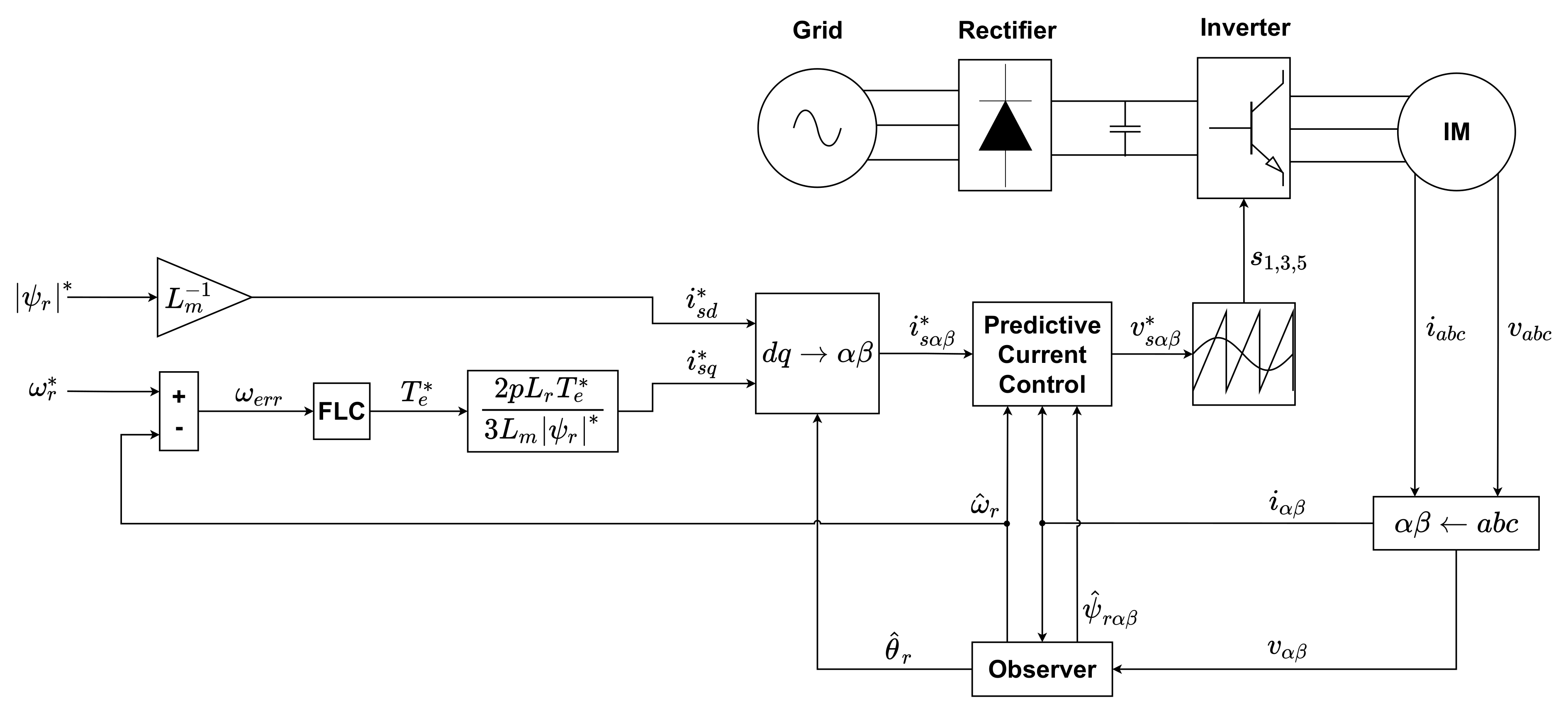
2. Induction Machine Model and Control Overview

The dynamic model of the induction machine is written in the stationary $\alpha \beta$-reference frame and it is shown by Equations (1)–(4), where J is the inertia constant of the machine, ${\omega }_r$ is the rotor shaft speed, p is the number of pole pairs, $T_e$ is electromechanical torque, and $T_l$ is load torque.

$$\begin{array}{c}{\mathit{v}}_{s\alpha \beta }={\mathit{R}}_s{\mathit{i}}_{s\alpha \beta }+\frac{\mathrm{d}}{\mathrm{d}t}{\mathit{\psi }}_{s\alpha \beta }\end{array}$$

(1)

$$\begin{array}{c}0={\mathit{R}}_r{\mathit{i}}_{r\alpha \beta }-{\mathit{J}}_{r}p{\omega }_r{\mathit{\psi }}_{r\alpha \beta }+\frac{\mathrm{d}}{\mathrm{d}t}{\mathit{\psi }}_{r\alpha \beta }\end{array}$$

(2)

$$\begin{array}{c}J\frac{\mathrm{d}}{\mathrm{d}t}{\omega }_r=T_e-T_l\end{array}$$

(3)

$$\begin{array}{c}{T}_e=\frac{3}{2}p({\psi }_{s\alpha }{i}_{s\beta }-{\psi }_{s\beta }{i}_{s\alpha })\end{array}$$

(4)

Equation (5) displays electrical quantities, where ${\mathit{v}}_{s\alpha \beta }$ represents the stator voltage vector, ${\mathit{i}}_{s\alpha \beta }$ and ${\mathit{i}}_{r\alpha \beta }$ represent the stator and rotor current vector, while ${\mathit{\psi }}_{s\alpha \beta }$ and ${\mathit{\psi }}_{r\alpha \beta }$ describe stator and rotor flux linkages.

$${\mathit{v}}_{s\alpha \beta }=\left[\begin{array}{c}{v}_{s\alpha }\\ v_{s\beta }\end{array}\right]{\mathit{i}}_{s\alpha \beta }=\left[\begin{array}{c}{i}_{s\alpha }\\ i_{s\beta }\end{array}\right]{\mathit{i}}_{r\alpha \beta }=\left[\begin{array}{c}{i}_{r\alpha }\\ i_{r\beta }\end{array}\right]{\mathit{\psi }}_{s\alpha \beta }=\left[\begin{array}{c}{\psi }_{s\alpha }\\ {\psi }_{s\beta }\end{array}\right]{\mathit{\psi }}_{r\alpha \beta }=\left[\begin{array}{c}{\psi }_{r\alpha }\\ {\psi }_{r\beta }\end{array}\right]$$

(5)

Electrical parameters are described by Equation (6), where ${\mathit{R}}_s$ and ${\mathit{R}}_r$ are the stator and rotor resistance matrices, while ${\mathit{J}}_r$ represents the rotation matrix.

$${\mathit{R}}_s=\left[\begin{array}{c}{R}_s\hspace{1em}0\\ 0\hspace{1em}{R}_s\end{array}\right]{\mathit{R}}_r=\left[\begin{array}{c}{R}_r\hspace{1em}0\\ 0\hspace{1em}{R}_r\end{array}\right]{\mathit{J}}_r=\left[\begin{array}{c}0\hspace{1em}-\\ 1\hspace{1em}0\end{array}\right]$$

(6)

Additionally, the relationship between fluxes and currents is described by Equations (7) and (8), but for a deeper understanding of the induction machine model, the reader is referred to [43].

$$\begin{array}{c}{\mathit{\psi }}_{s\alpha \beta }=L_s{\mathit{i}}_{s\alpha \beta }+L_m{\mathit{i}}_{r\alpha \beta }\end{array}$$

(7)

$$\begin{array}{c}{\mathit{\psi }}_{r\alpha \beta }=L_r{\mathit{i}}_{r\alpha \beta }+L_m{\mathit{i}}_{s\alpha \beta }\end{array}$$

(8)

Model predictive control has attracted research interest in recent years, as seen in papers such as [44,45,46]. This being the case, the control method that is being modified in this paper is PCC for an induction machine, which falls into the family of model predictive control structures. In the following text, it is explained how it works.

Firstly, a discrete state space model for computing the current prediction $i_{s\alpha \beta }[k+1]$ is formed by selecting stator currents $i_{s\alpha \beta }\left[k\right]$ and rotor fluxes ${\psi }_{r\alpha \beta }\left[k\right]$ as state variables. Equation (9) represents the final expression to calculate the current predictions, where $\sigma =1-\frac{L_m^2}{L_s{L}_r}$ represents the leakage inductance factor, ${\tau }_r=\frac{L_r}{R_r}$ represents the rotor time constant, and $T_s$ represents the discretization sampling time.

$$\begin{array}{cc}\hfill \left[\begin{array}{c}\hfill i_{s\alpha }[k+1]\\ \hfill i_{s\beta }[k+1]\end{array}\right]& =\left[\begin{array}{cccc}1-\frac{(R_s+\frac{L_m^2}{L_r{\tau }_r})T_s}{\sigma L_s}& \hfill 0\hfill & \frac{L_m{T}_s}{\sigma L_s{L}_r{\tau }_r}& \frac{L_{m}p{\omega }_r{T}_s}{\sigma L_s{L}_r}\\ \hfill 0\hfill & 1-\frac{(R_s+\frac{L_m^2}{L_r{\tau }_r})T_s}{\sigma L_s}\hfill & \hfill -\frac{L_{m}p{\omega }_r{T}_s}{\sigma L_s{L}_r}& \frac{L_m{T}_s}{\sigma L_s{L}_r{\tau }_r}\hfill \end{array}\right]\hspace{1em}\left[\begin{array}{c}{i}_{s\alpha }\left[k\right]\\ i_{s\beta }\left[k\right]\\ \hfill {\psi }_{r\alpha }\left[k\right]\\ \hfill {\psi }_{r\beta }\left[k\right]\end{array}\right]\\ & +\left[\begin{array}{cc}\frac{T_s}{\sigma L_s}& \hfill 0\\ \hfill 0& \frac{T_s}{\sigma L_s}\hfill \end{array}\right]\hspace{1em}\left[\begin{array}{c}{v}_{s\alpha }\left[k\right]\\ \hfill v_{s\beta }\left[k\right]\end{array}\right]\hfill \end{array}$$

(9)

Equation (10) represents the cost function that is used to derive the control law by minimizing the squared error between reference currents $i_{\alpha }^{*}\left[k\right]$, $i_{\beta }^{*}\left[k\right]$ and current predictions. By inserting (9) into (10) and solving (11), the optimal voltage vector ${\mathit{v}}_{\alpha \beta }^{*}$ can be obtained to minimize the cost function and drive the machine in the desired state.

$$\mathit{G}=\left[\begin{array}{c}{g}_{\alpha }\\ g_{\beta }\end{array}\right]=\left[\begin{array}{c}{(i_{\alpha }^{*}\left[k\right]-i_{\alpha }[k+1])}^2\\ {(i_{\beta }^{*}\left[k\right]-i_{\beta }[k+1])}^2\end{array}\right]$$

(10)

$$\frac{\partial \mathit{G}}{{\partial \mathit{v}}_{\alpha \beta }}=0$$

(11)

Equation (12) represents the solution of (11), which is used as a control law.

$$\begin{array}{cc}\hfill {\mathit{v}}_{\alpha \beta }^{*}[k+1]& =\left[\begin{array}{cccc}{R}_s+\frac{L_m^2}{L_r{\tau }_r}-\frac{\sigma L_s}{T_s}& \hfill 0\hfill & -\frac{L_m}{L_r{\tau }_r}\hfill & \hfill -\frac{L_{m}p{\omega }_r}{L_r}\\ \hfill 0\hfill & R_s+\frac{L_m^2}{L_r{\tau }_r}-\frac{\sigma L_s}{T_s}\hfill & \hfill \frac{L_{m}p{\omega }_r}{L_r}& -\frac{L_m}{L_r{\tau }_r}\hfill \end{array}\right]\left[\begin{array}{c}{i}_{s\alpha }\left[k\right]\\ i_{s\beta }\left[k\right]\\ {\psi }_{r\alpha }\left[k\right]\\ {\psi }_{r\beta }\left[k\right]\end{array}\right]\hfill \\ & +\left[\begin{array}{cc}\frac{\sigma L_s}{T_s}& \hfill 0\\ 0\hfill & \frac{\sigma L_s}{T_s}\end{array}\right]\left[\begin{array}{c}{i}_{s\alpha }^{*}\left[k\right]\\ i_{s\beta }^{*}\left[k\right]\end{array}\right]\hfill \end{array}$$

(12)

Reference current value $i_{\alpha }^{*}\left[k\right]$ is calculated from the desired rotor flux of the machine, while reference current $i_{\beta }^{*}\left[k\right]$ is generated by the FLC acting as a speed controller. Figure 1 represents the final topology of the control structure, and more details about the PCC structure can be found in [47].

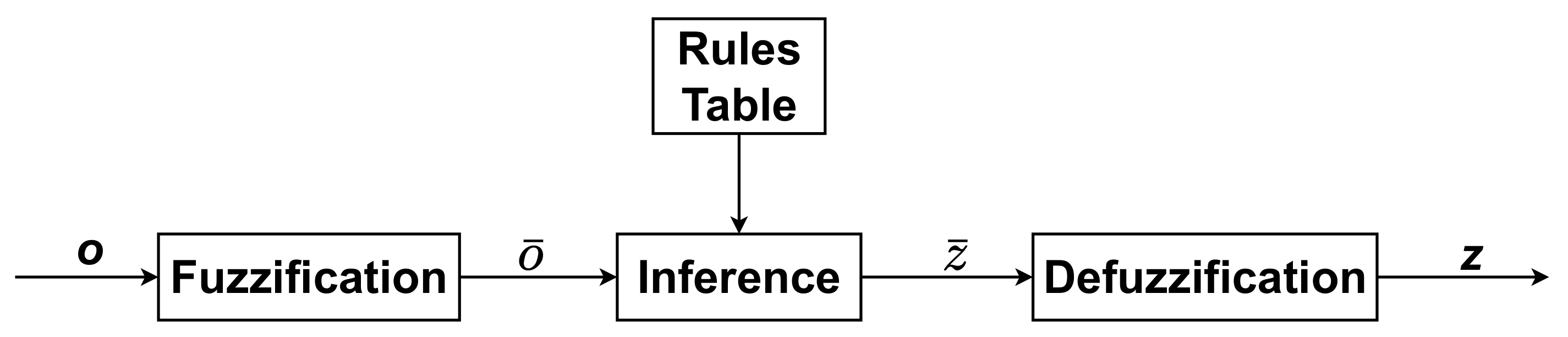
3. Fuzzy Logic Controller

The fuzzy inference system block diagram is shown in Figure 2. It represents the computation steps used to transfer inputs to the fuzzy system into control outputs used for generating reference values for induction machine predictive current control. First, input values are turned into fuzzy values by the process of fuzzification. These fuzzy values are calculated using predefined membership functions. The following text explains the selection of input and output variables and membership functions that are to be optimized for induction machine speed control.

3.1. Input and Output of Fuzzy Controller

Input variables to the fuzzy controller are chosen to be the speed tracking error ${\omega }_{err}$ and its derivative ${\dot{\omega }}_{err}$, while the output is defined as fuzzy error $f_{err}$. All relevant vectors and sets that will be used are: real valued input vector $\mathit{o}$, input linguistic variable vector $\overline{\mathit{o}}$, and input linguistic value sets ${\overline{O}}_i$, where i represents the input ordinal number. Regarding the output, $\mathit{z}$ represents the real valued output vector, $\overline{\mathit{z}}$ represents the output linguistic variable vector, and $\overline{Z}$ represents the output linguistic value set. Established vectors and sets are defined as follows:

• $\mathit{o}=[{\omega }_{err}\hspace{1em}{\dot{\omega }}_{err}]$,
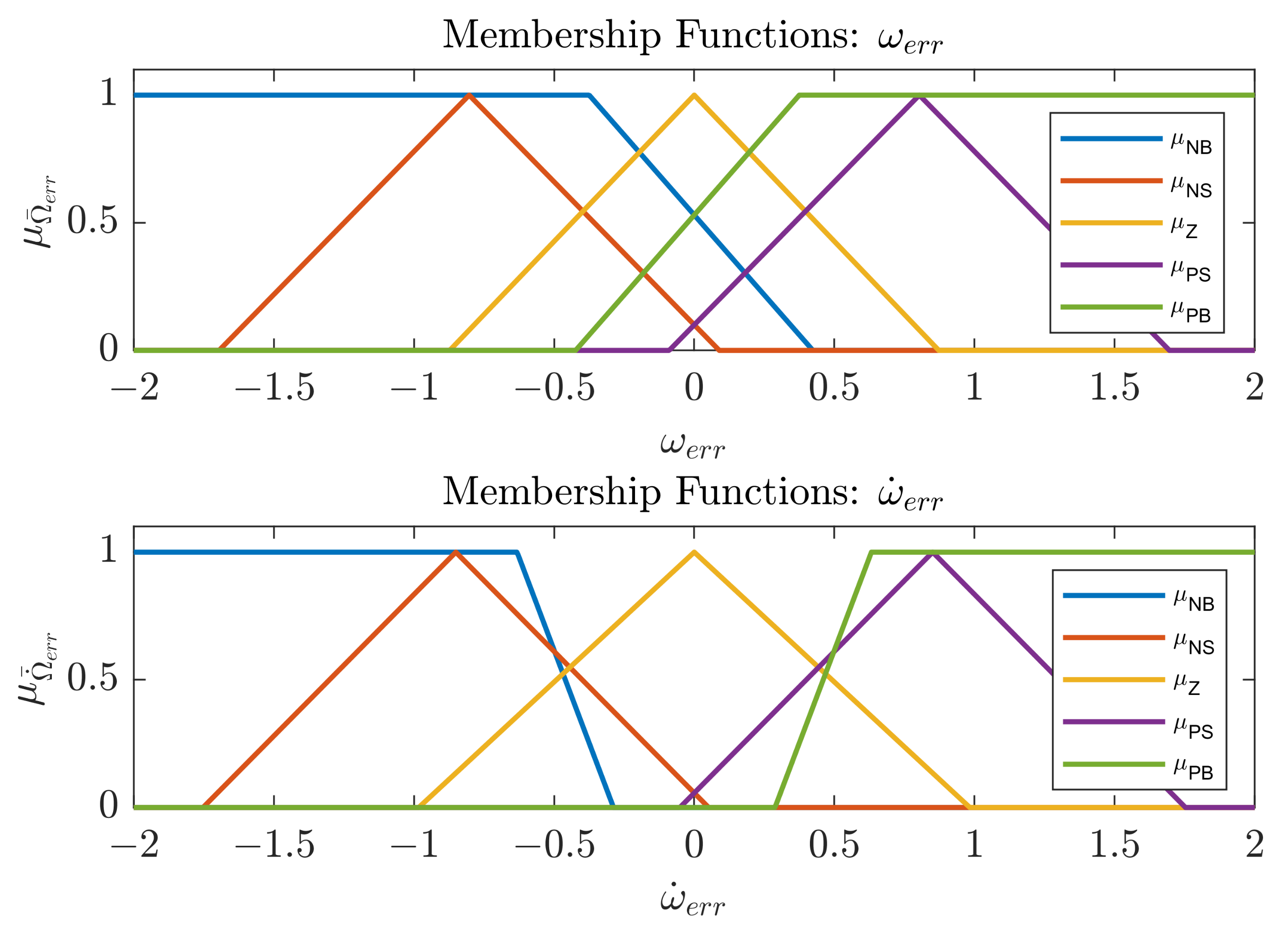
• $\overline{\mathit{o}}=$ ["Speed Error" "Speed Error Derivative"],
• ${\overline{O}}_1={\overline{O}}_2=$ {"Negative Big", "Negative Small", "Zero", "Positive Small", "Positive Big"},
• $\mathit{z}=\left[f_{err}\right]$,
• $\overline{\mathit{z}}=$ ["Fuzzy Error"],
• $\overline{Z}=$ {"Negative", "Zero", "Positive"}.

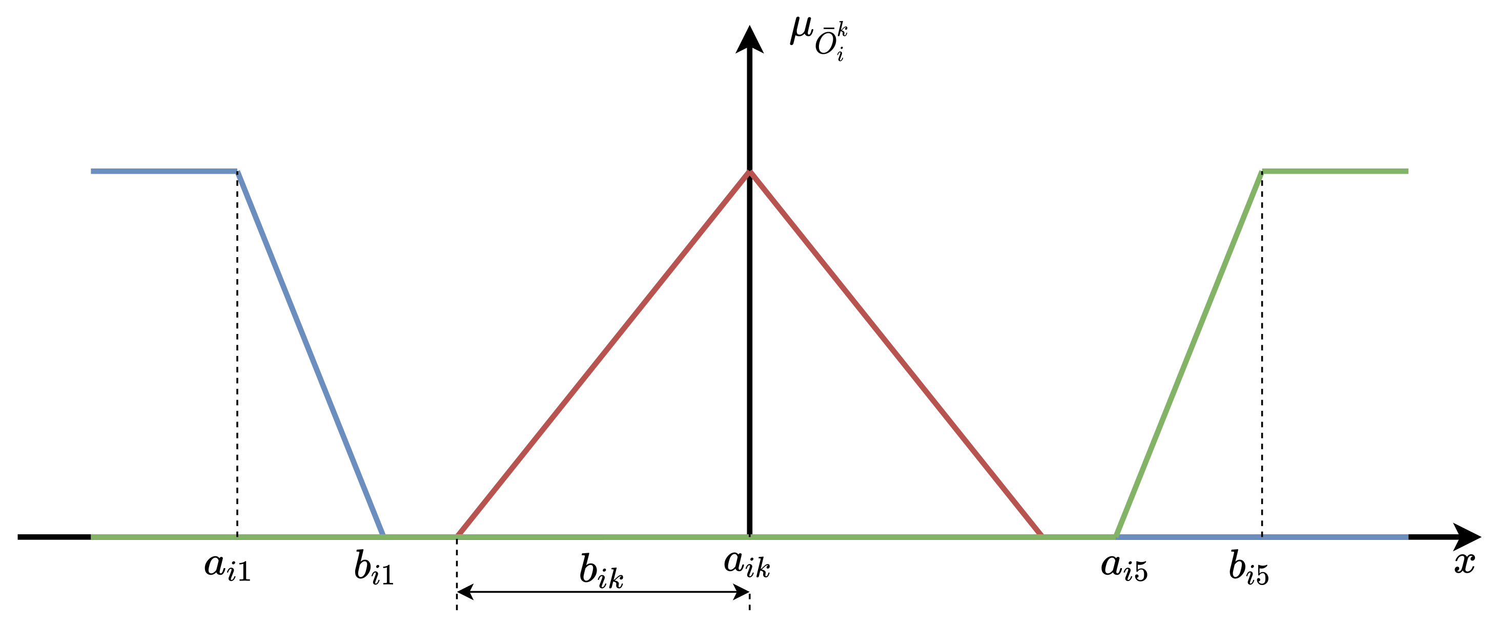
3.2. Input Membership Functions

Membership functions are structured for $i\mathrm{th}$ input linguistic variable ${\overline{o}}_i$ and $k\mathrm{th}$ possible linguistic value ${\overline{O}}^k$. Their structure depends on the observed linguistic variable and its linguistic value. Equations (13)–(15) represent the membership function definitions for all the possible combinations of index values i and superscript values k. It can be seen that they are unit piecewise linear and defined using only two parameters, $a_{ik}$ and $b_{ik}$. Figure 3 gives a deeper insight into the membership functions and their parameters.

$${\mu }_{{\overline{O}}_i^k}\left(o_i\right)=max\left[\left(1-\left|\frac{a_{ik}-o_i}{b_{ik}}\right|\right),0\right],i\in \{1,2\},k\in \{2,3,4\}$$

(13)

$${\mu }_{{\overline{O}}_i^k}\left(o_i\right)=\left\{\begin{array}{c}1,o_i<a_{ik}\hfill \\ 0,o_i>b_{ik}\hfill \\ \frac{a_{ik}-o_i}{b_{ik}-a_{ik}}+1,a_{ik}\le o_i\le b_{ik}\hfill \end{array}\right.i\in \{1,2\},k=1$$

(14)

$${\mu }_{{\overline{O}}_i^k}\left(o_i\right)=\left\{\begin{array}{c}0,o_i<a_{ik}\hfill \\ 1,o_i>b_{ik}\hfill \\ \frac{o_i-a_{ik}}{b_{ik}-a_{ik}},a_{ik}\le o_i\le b_{ik}\hfill \end{array}\right.i\in \{1,2\},k=5$$

(15)

The fact that there are only two parameters required for membership function definition offers simplicity of implementation and can be exploited in the optimization procedure of the fuzzy speed controller, as is seen in the following sections. The next step is to obtain the controller output value through the process of fuzzy inference and defuzzification.

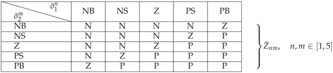
3.3. Fuzzy Inference

In control, it is common practice to follow the convention shown in

Table 1. Fuzzy rules.

of [10] or

Table 2. Optimization search area.

Parameter	Value (${\mathit{\theta }}^{\mathit{min}}$)	Value (${\mathit{\theta }}^{\mathit{max}}$)
$a_{ik}$, $b_{ik}$	0	1
$a_P$, $b_P$,$c_P$	0	100
$B_e$, $B_{ce}$	0.000001	10,000
$K_{Pf}$	0	10,000
$K_{If}$	0	100,000

of [40] for fuzzy rule table construction, where an equal number of input and output linguistic values exist in each set ${\overline{O}}_i$ and $\overline{Z}$. In this paper, however, this convention is not followed since the input linguistic value set contains five elements, while the output linguistic value set consists of three elements. This is done to reduce the number of decision variables in the optimization problem and speed up the overall computation. Table 1 represents the fuzzy rule table that is used in this paper. Abbreviations are used to represent the linguistic values: N for Negative, P for Positive, Z for Zero, S for Small, and B for Big. Rules are interpreted as follows: "if Speed Error is Negative-Big and Speed Error Derivative is Negative-Big, then Fuzzy Error is Negative", and so on.

Using Table 1, it is possible to calculate the rule firing strength matrix $\mathit{W}$, shown in Equation (16), whose elements are calculated using Equation (17). This matrix is used to obtain the output control value in the defuzzification process.

$$\begin{array}{c}\mathit{W}=\left[\begin{array}{ccc}{w}_{11}& \cdots & w_{1m}\\ ⋮& \ddots & ⋮\\ w_{n1}& \cdots & w_{nm}\end{array}\right]\end{array}$$

(16)

$$w_{nm}=min({\mu }_{{\overline{O}}_1^n}\left(o_1\right),{\mu }_{{\overline{O}}_2^m}\left(o_2\right)),n,m\in [1,5]$$

(17)

3.4. Defuzzification

Defuzzification is the final step to obtain the real output value, and in this paper, the Takagi–Sugeno method is used because it is simple to implement and fast for computation. It is executed by forming rule output level matrix $\mathit{H}$, shown in Equation (18). Elements of matrix $\mathit{H}$ are calculated using Equation (19). This equation is structured for each element in matrix $\mathit{H}$ and its coefficients depend on the output linguistic value ${\overline{Z}}_{nm}$ defined by Table 1.

$$\begin{array}{c}\mathit{H}=\left[\begin{array}{ccc}{h}_{11}& \cdots & h_{1m}\\ ⋮& \ddots & ⋮\\ h_{n1}& \cdots & h_{nm}\end{array}\right]\end{array}$$

(18)

$$\begin{array}{c}{h}_{nm}=c_{nm}{o}_1+d_{nm}{o}_2+e_{nm}\\ c_{nm}=\left\{\begin{array}{c}{c}_N,{\overline{Z}}_{nm}=N\hfill \\ c_Z,{\overline{Z}}_{nm}=Z\hfill \\ c_P,{\overline{Z}}_{nm}=P\hfill \end{array}\right.\hspace{1em}{d}_{nm}=\left\{\begin{array}{c}{d}_N,{\overline{Z}}_{nm}=N\hfill \\ d_Z,{\overline{Z}}_{nm}=Z\hfill \\ d_P,{\overline{Z}}_{nm}=P\hfill \end{array}\right.\hspace{1em}{e}_{nm}=\left\{\begin{array}{c}{e}_N,{\overline{Z}}_{nm}=N\hfill \\ e_Z,{\overline{Z}}_{nm}=Z\hfill \\ e_P,{\overline{Z}}_{nm}=P\hfill \end{array}\right.\\ n,m\in [1,5]\end{array}$$

(19)

Defuzzified output controller value z is calculated from matrices $\mathit{W}$ and $\mathit{H}$, as shown in Equation (20).

$$z=\frac{{\displaystyle \sum _{i=n}^5}{\displaystyle \sum _{m=1}^5}{w}_{nm}{h}_{nm}}{{\displaystyle \sum _{i=n}^5}{\displaystyle \sum _{m=1}^5}{w}_{nm}}$$

(20)

The final topology of the FLC that is used in the paper is shown in Figure 4. It can be seen that there are four additional parameters: $B_e$ and $B_{ce}$ are base values, which are used to scale the inputs of the fuzzy controller, since input membership functions are chosen to be unit piecewise functions. $K_{Pf}$ and $K_{If}$ serve as proportional and integral gains on the produced fuzzy error.

It can be seen from Figure 1 that the described fuzzy logic controller is used as a speed controller to generate torque reference, which implicitly generates the reference $\beta$-current component through some scaling and reference frame transformation. Based on the selected input membership functions, output level functions, and base and gain values of the controller, there are 33 parameters, represented by vector $\mathit{\theta }$ in Equation (21), that need to be tuned to accurately control the drive. Vector $\mathit{\theta }$ is also called a decision variable vector that is used in the fuzzy controller optimization procedure, which is explained in the following section.

$$\begin{array}{cc}\hfill \mathit{\theta }& =\{a_{11}\cdots a_{ik},b_{11}\cdots b_{ik},c_N,c_Z,c_P,d_N,d_Z,d_P,e_N,e_Z,e_P,B_e,B_{ce},K_{Pf},K_{If}\}\hfill \\ \hfill & =\{{\theta }_1,{\theta }_2,\cdots ,{\theta }_{33}\},k\in [1,5],i\in \{1,2\}\hfill \end{array}$$

(21)

4. Optimization of Fuzzy Logic Controller

In the following text, the optimization procedure of the FLC is explained. The problem statement is given, the objective function structure with decision variables and their boundaries is selected, and the optimization tool is described.

4.1. Problem Statement

In the proposed control method, FLC is employed as a speed controller that produces a torque reference for PCC of an induction machine. The reference torque must change in a timely manner to produce minimal speed tracking error and have a minimal amount of overshoot so that it does not stress the rotor shaft. To meet these demands, optimal FLC parameters must be calculated. FLC is defined by a large number of parameters, and to find the optimal combination of them, optimization must be employed. Parameters calculated in the optimization process highly depend on the criteria used to calculate the objective function value. The following text provides insight into how different criteria affect the final results. By finding the correct criterion, optimal parameters that produce the best induction machine drive performance can be obtained.

4.2. Objective Function

To optimize FLC, a number of objective functions are explored and the one that produces the best results (which are small speed tracking error and small torque overshoot) is further analyzed. These are Integral Absolute Error, Integral Squared Error, Integral Time Absolute Error, and Integral Time Squared Error, represented by Equation (22), where $\mathit{\theta }$ represents the decision variable vector.

$$\begin{array}{cc}\hfill f_{IAE}=f_1\left({\omega }_{err}\left(\mathit{\theta }\right)\right)& ={\int }_0^{\infty }\left|{\omega }_{err}\left(\mathit{\theta }\right)\right|dt\hfill \\ \hfill f_{ISE}=f_2\left({\omega }_{err}\left(\mathit{\theta }\right)\right)& ={\int }_0^{\infty }{\omega }_{err}^2\left(\mathit{\theta }\right)dt\hfill \\ \hfill f_{ITAE}=f_3\left({\omega }_{err}\left(\mathit{\theta }\right)\right)& ={\int }_0^{\infty }\left|{\omega }_{err}\left(\mathit{\theta }\right)\right|tdt\hfill \\ \hfill f_{ITSE}=f_4\left({\omega }_{err}\left(\mathit{\theta }\right)\right)& ={\int }_0^{\infty }{\omega }_{err}^2\left(\mathit{\theta }\right)tdt\hfill \end{array}$$

(22)

${\omega }_{err}\left(\mathit{\theta }\right)$ represents the speed tracking error calculated as the difference between speed reference ${\omega }_r^{*}$ and induction machine speed response ${\omega }_r\left(\mathit{\theta }\right)$, as shown in Equation (23). These responses are calculated through Simulink simulation of a drive system, which is shown in Figure 1. In the optimization procedure, the inverter and observer blocks are omitted from the simulation to speed up the computation. The parameters of the induction machine that is controlled are given in

Table A1. Induction machine and simulation parameters.

Parameter		Value
Stator resistance	$R_s$ ($\Omega$)	1.1507
Rotor resistance	$R_r$ ($\Omega$)	1.0107
Stator inductance	$L_s$ ($\mathrm{H}$)	0.1315
Rotor inductance	$L_r$ ($\mathrm{H}$)	0.1315
Mutual inductance	$L_m$ ($\mathrm{H}$)	0.126
Pole pairs	p	2
Inertia	J ($\mathrm{k}\mathrm{g}$${\mathrm{m}}^2$)	0.129
Simulation step size	$T_s$ ($\mathrm{s}$)	${10}^{-4}$
Solver	Fixed-step	Runge–Kutta

in Appendix A, along with relevant simulation parameters.

$${\omega }_{err}\left(\mathit{\theta }\right)={\omega }_r^{*}-{\omega }_r\left(\mathit{\theta }\right)$$

(23)

Simulated dynamics of a drive system are shown in Figure 5. It can be seen in Figure 5a that the speed reference is a function that is ramping from 0 to 1432.5 rpm during a 2 s period starting at 0.2 s of the simulation. Nominal load torque of 27 Nm is applied at the 3rd second of the simulation and it is constant till the end of the simulation, as can be seen from Figure 5b. Figure 5c represents the required machine torque profile calculated using Equation (24).

$$T_e=J\frac{\mathrm{d}}{\mathrm{d}t}{\omega }_r^{*}+T_l$$

(24)

It can be seen from Figure 5c that torque overshoot can appear at the beginning of ramping (OS1) and loading instance (OS3), while undershoot can appear at the end of ramping (OS2). Total torque overshoot is calculated by Equation (25), and it is used to construct another set of objective functions, represented by Equation (26), where w represents a weighing factor.

$$f_{OS}=\left|OS1\right|+\left|OS2\right|+\left|OS3\right|$$

(25)

$$\begin{array}{cc}\hfill f_{IAE+OS}=f_5\left({\omega }_{err}\left(\mathit{\theta }\right)\right)& =f_1\left({\omega }_{err}\left(\mathit{\theta }\right)\right)+w·f_{OS}\hfill \\ \hfill f_{ISE+OS}=f_6\left({\omega }_{err}\left(\mathit{\theta }\right)\right)& =f_2\left({\omega }_{err}\left(\mathit{\theta }\right)\right)+w·f_{OS}\hfill \\ \hfill f_{ITAE+OS}=f_7\left({\omega }_{err}\left(\mathit{\theta }\right)\right)& =f_3\left({\omega }_{err}\left(\mathit{\theta }\right)\right)+w·f_{OS}\hfill \\ \hfill f_{ITSE+OS}=f_8\left({\omega }_{err}\left(\mathit{\theta }\right)\right)& =f_4\left({\omega }_{err}\left(\mathit{\theta }\right)\right)+w·f_{OS}\hfill \end{array}$$

(26)

Equation (27) represents the optimal decision variable values ${\mathit{\theta }}_i^{opt}$, obtained by the minimization of the previously formulated objective functions, where S represents a constraint on the optimization search area, while index i represents the ordinal number of objective functions that was used in the optimization procedure. In the following text, decision variable selection is further explained, along with the imposed constraints.

$$\begin{array}{c}{\mathit{\theta }}_i^{opt}=\underset{\mathit{\theta }\in S\subset \mathbb{R}}{argmin}\left[f_i\left({\omega }_{err}\left(\mathit{\theta }\right)\right)\right],i\in [1,8]\\ S\in [{\mathit{\theta }}^{min},{\mathit{\theta }}^{max}]\end{array}$$

(27)

4.3. Decision Variables

Fuzzy controller parameters (membership function and output level function parameters, base and gain values) lead to the decision variable vector $\mathit{\theta }$, as was previously established by Equation (21) in the previous section. Some simplification measures can be taken to reduce the number of elements in the vector: it can be concluded that the controller must have the same output in absolute value for negative and positive inputs. This means that only membership functions corresponding to positive linguistic values can be defined, and the opposites can be used for the negative counterparts. This reduces the number of decision variables regarding input membership functions from 20 to 10. The same is true for the rule output level functions. Coefficients $a_Z$, $b_Z$ and $c_Z$ from Equation (19) can be set to zero and only coefficients regarding positive linguistic values can be defined, which reduces the number of variables from 9 to 3. This means that the final vector of decision variables $\mathit{\theta }$ contains only 17 instead of 33 elements. Table 2 represents the limits of the optimization search area.

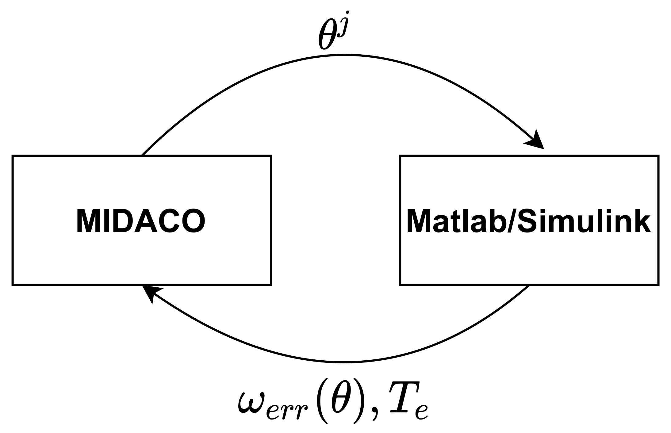
4.4. MIDACO Optimizer

In this paper, the authors use the MIDACO solver, which stands for “Mixed Integer Distributed Ant Colony Optimization”, which is one of many metaheuristic methods for global optimum search, inspired by nature. It is chosen because it is easy to use and works well with a large number of decision variables and can also work in co-simulation with the Matlab environment. Out of the many settings that the solver offers, it only requires settings for decision variable limits and the start point of the search. Figure 6 represents the co-simulation between Matlab/Simulink and MIDACO that is executed to optimize the fuzzy controller parameters, where ${\mathit{\theta }}^j$ represents the decision variable values of the current evaluation.

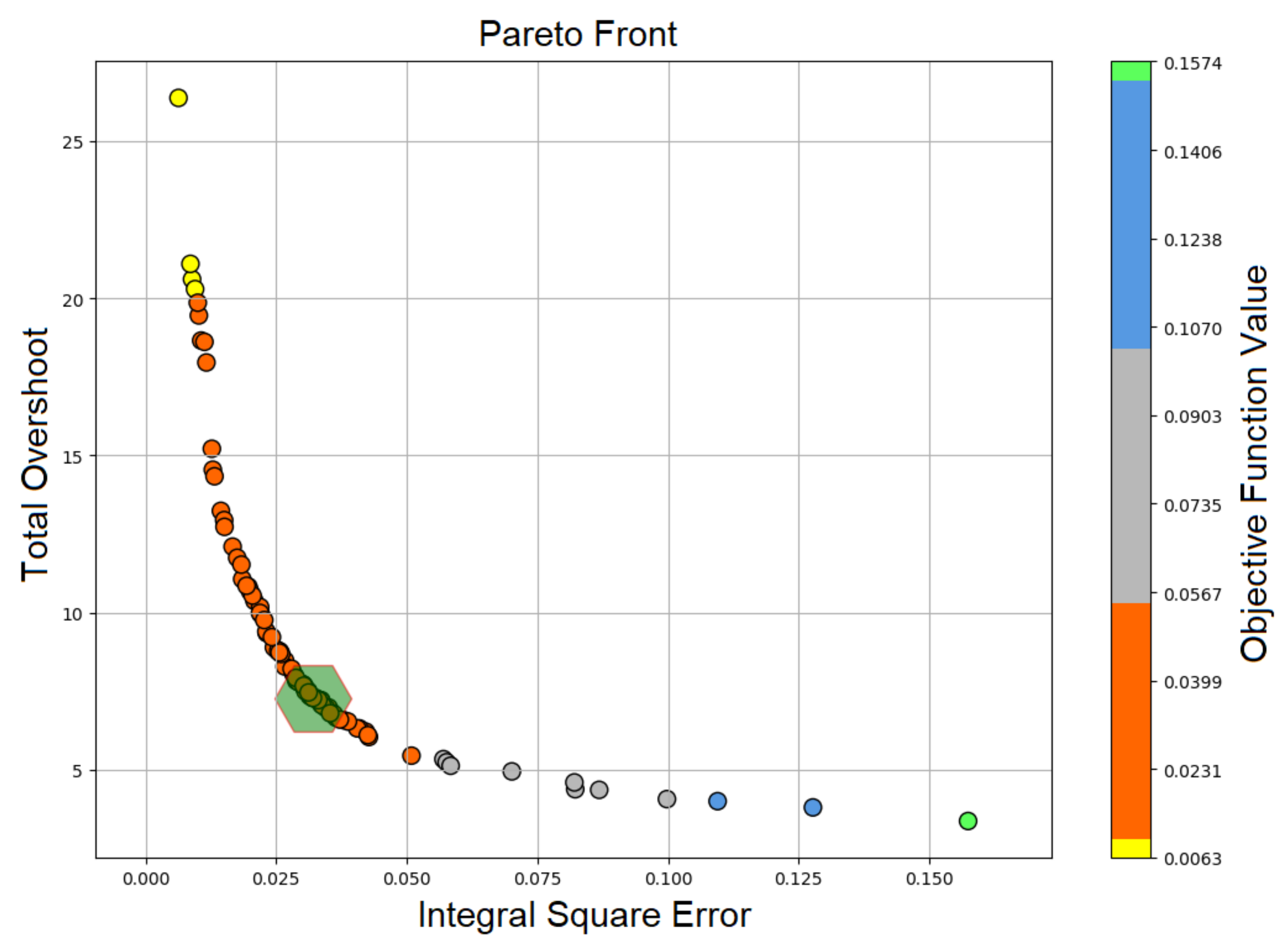
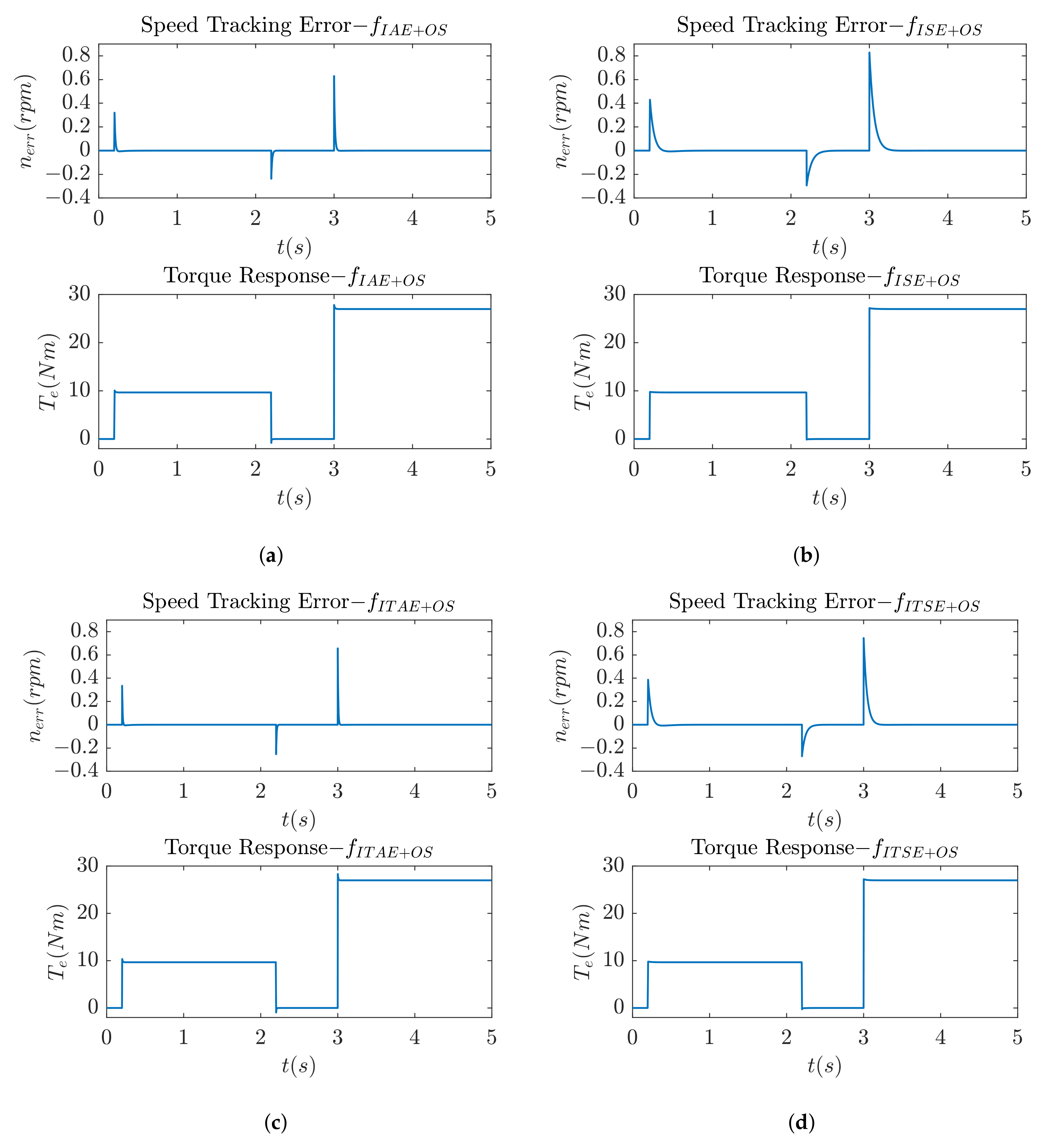
5. Optimization Results

In this section, the optimization results, obtained by criteria from Equations (22), (25), and (26), are presented. Figure 7 shows the speed and torque responses that are obtained by using only criteria from Equation (22). It can be seen that the dynamics of the drive system have almost no impact on the speed response; in other words, the speed response has only around 0.2 rpm maximum tracking error and a fast settling time, but when observing the torque response, an unacceptable overshoot of around 20 Nm is observed. The reason for the large overshoot is the fact that the speed error is the only criterion for the optimization. To keep it at its lowest value, large control action is required at every instance when the speed diverges from the reference value. Since there is no criterion that would limit or penalize the torque, optimized parameters allow this kind of behavior. An attempt is made to remedy this problem with a multi-objective optimization approach. The first objective is selected as $f_{ISE}$ from Equation (22) and the second as overshoot from Equation (25). Figure 8 represents the optimization result in the form of a Pareto front, where the x-axis represents the $f_{ISE}$ value and the y-axis represents the total overshoot value.

Depending on the application, a range of solutions are available to choose from, and they are represented by the circles in the graph. The green hexagon in the figure is the area of the Pareto front that the optimizer selected a solution from, and Figure 9 represents the system response produced by its parameters.

It can be seen from Figure 9 that the overshoot in the torque response is greatly reduced. To obtain the unique solution that offers the best system response, criteria from Equation (26) are investigated.

Figure 10 represents the speed and torque responses of the criteria from Equation (26) with the weighing factor of value 10. It can be seen that the torque overshoot is greatly reduced, while preserving a good speed tracking response.

To summarize, nine different optimization procedures are conducted for nine different types of objective functions.

Table 3. Optimization results.

Optimization Procedure	Objective Function	Max Torque Overshoot (Nm)	Max Speed Tracking Error (rpm)
1	$f_{IAE}$	24.34	0.25
2	$f_{ISE}$	23.80	0.26
3	$f_{ITAE}$	21.28	0.28
4	$f_{ITSE}$	22.23	0.26
5 (multi-objective)	$f_1=f_{ISE},f_2=f_{OS}$	2.28	0.40
6	$f_{IAE+OS}$	0.84	0.63
7	$f_{ISE+OS}$	0.20	0.83
8	$f_{ITAE+OS}$	1.34	0.66
9	$f_{ITSE+OS}$	0.24	0.75

shows relevant metrics for each optimization procedure.

It can be seen from the results that single-objective optimizations that utilize objective functions $f_{ISE+OS}$ and $f_{ITSE+OS}$ produce the best results regarding torque overshoot, while keeping the speed tracking error below 1 rpm. Even though they do not differ significantly, the $f_{ISE+OS}$ criterion produces slightly better results, which is why it was chosen to be further investigated. Figure 11 shows the optimized membership functions and

Table 4. Gain and output level function coefficient values obtained by optimization.

Parameter	Value
$B_e$	6049.6
$B_{ce}$	3212.6
$K_{Pf}$	6076.7
$K_{If}$	98,680.5
$a_P$	77.5
$b_P$	51.66
$c_P$	94.78

shows the optimized gain and output level function coefficient values for the $f_{ISE+OS}$ criterion.

It should be noted that coefficients $a_N$, $b_N$ and $c_N$ have opposite values to their positive counterparts.

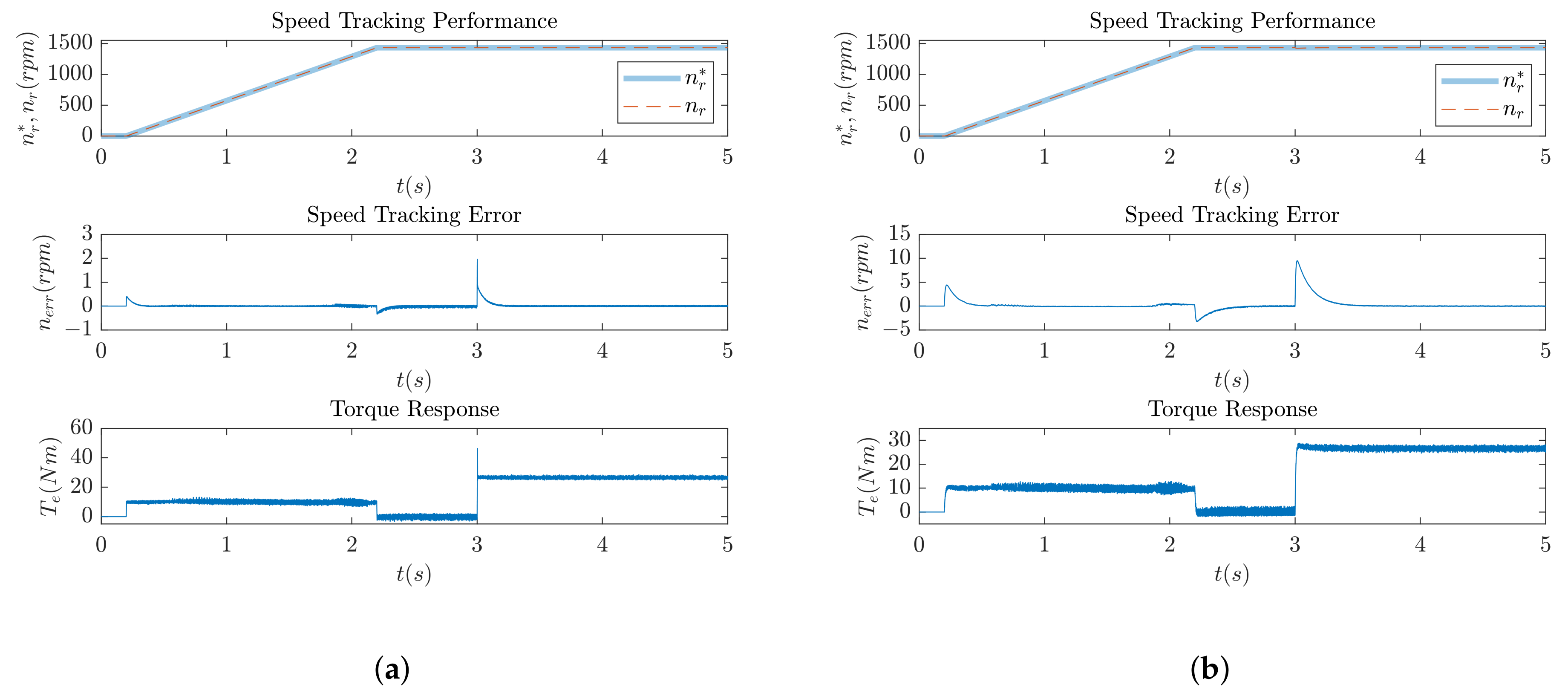
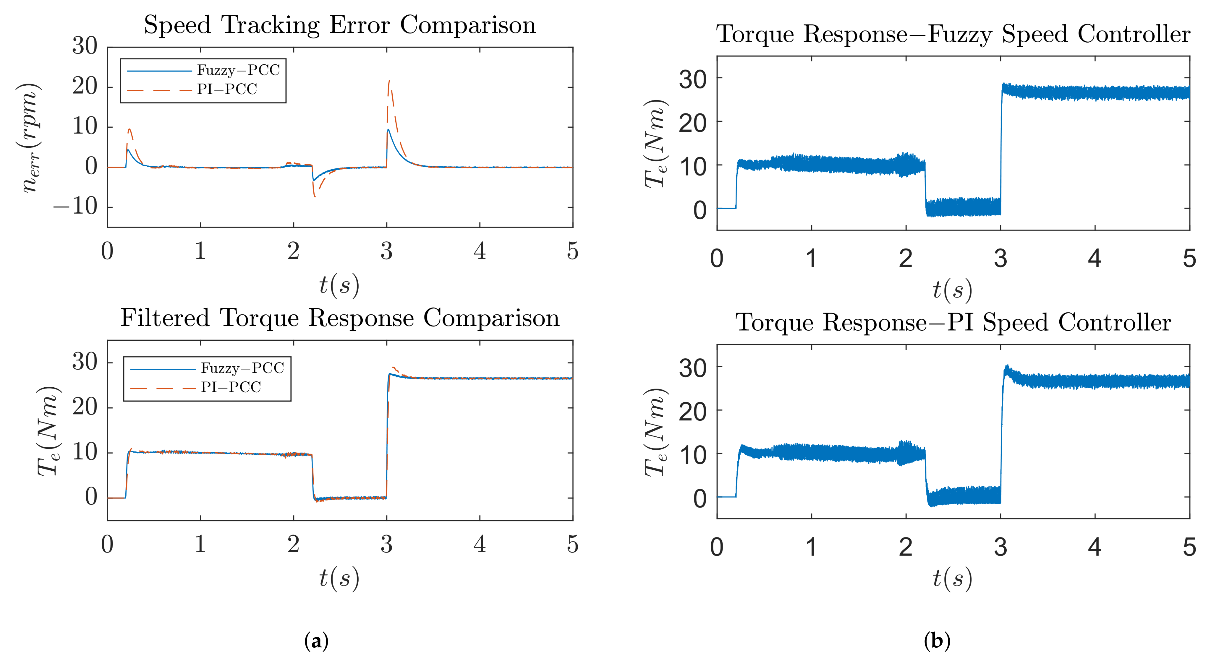
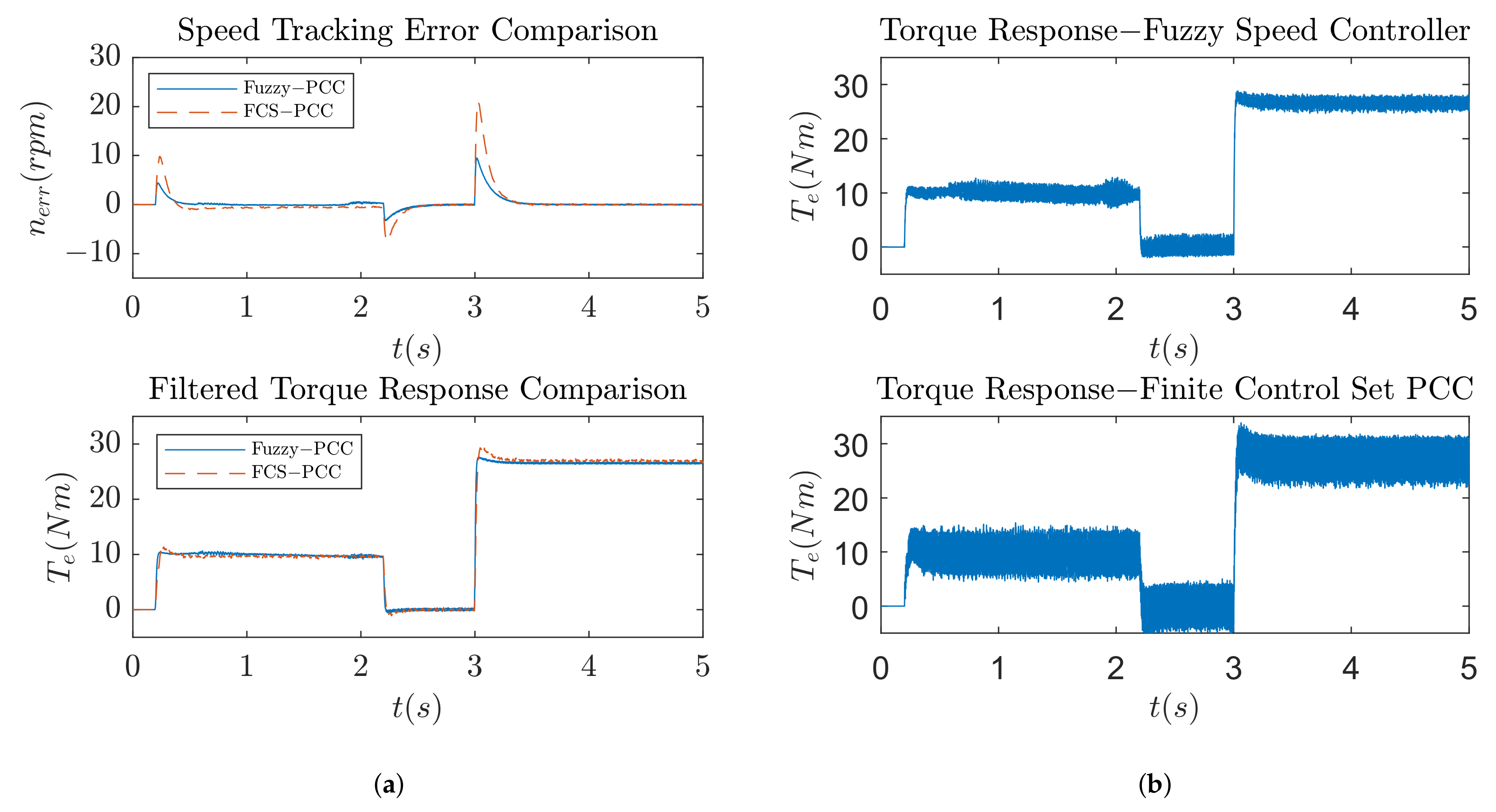
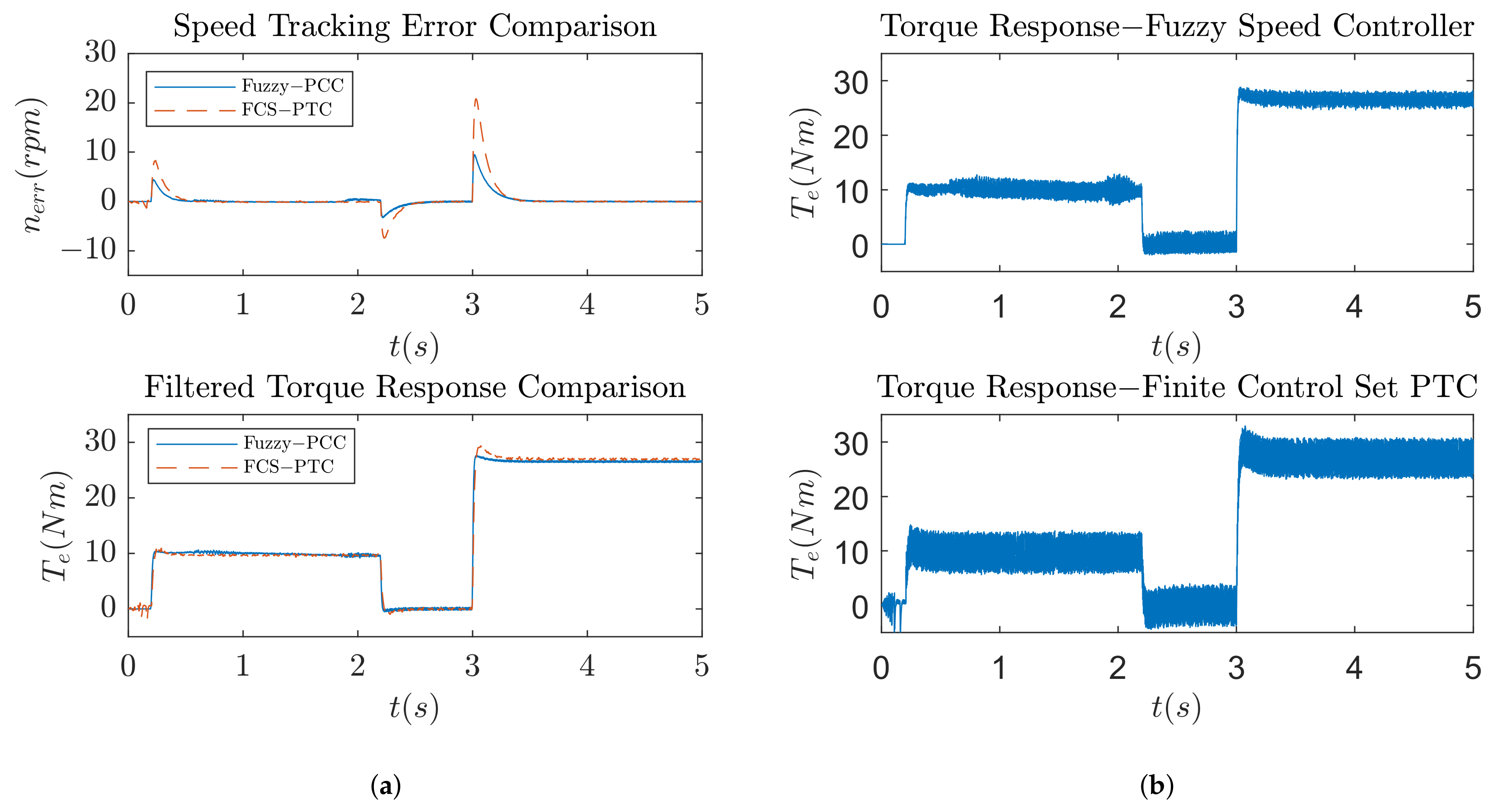
6. Control System Performance

In this section, a full simulation with the drive, inverter, and observer is evaluated. Control parameters used for the fuzzy controller are the ones obtained by the $f_{ISE+OS}$ criterion in the optimization procedure. A block diagram of the simulated control method is shown in the Figure 1. From the Figure 12a it can be seen that optimized controller parameters produce great speed tracking with maximum tracking error of only 2 rpm, but still produce large torque overshoot at the loading instance. By reducing the proportional and integral gain of the fuzzy logic controller, it is possible to adjust the response and remedy this problem. Figure 12b shows the performance of the system with reduced gains—in this case, $K_{Pf}=500$ and $K_{If}=4000$. It can be seen that the torque overshoot is greatly improved, while the speed response is slightly affected, but the system still offers a small maximum tracking error of around 10 rpm. In the following section, a comparison with several conventional model predictive control methods will be performed.

7. Discussion

The optimization procedures conducted in the study show improvements in the speed tracking response of the induction machine drive. Figure 9 shows the improvement when using multi-objective optimization over single-objective optimization, whose results are represented by Figure 7. The reason for the improvement is that torque overshoot penalization is added via a second objective function, and the result is a Pareto front that offers a range of solutions to chose from, based on the application. Figure 10 shows further improvements: single-objective optimization is used and torque overshoot can be arbitrarily penalized using a weighing factor, which results in the smallest amount of overshoot and good speed tracking behavior. A comparison between the proposed method and PCC method that utilizes a classic PI speed controller is shown in Figure 13. In Figure 13a, it can be seen that the speed response is greatly improved, with a much smaller value of maximum speed tracking error but similar settling time. Torque responses are filtered to better represent overshoots, and as can be seen from the same figure, the optimized fuzzy speed controller produces less torque overshoot than the classic PI controller. The reason for the better response is the fact that the fuzzy speed controller acts on the speed tracking error derivative along with the speed tracking error. The speed tracking error derivative can be understood as a form of torque estimation which increases control action in the instances when the torque is changing. The classic PI controller does not have this advantage, since it only acts on the speed tracking error. Figure 13b shows the unfiltered torque response for both methods. It can be seen that the chattering produced by both methods is in the same range. To further confirm the effectiveness of the method, two more comparisons with different predictive control methods are conducted. Figure 14 shows a comparison of the proposed method with Finite Control Set-Predictive Current Control (FCS-PCC), while Figure 15 represents a comparison of the proposed method with Finite Control Set-Predictive Torque Control (FCS-PTC). To gain an understanding of both methods, the reader is referred to [48,49]. It can be seen from Figure 14a and Figure 15a that the speed tracking error and filtered torque responses are similar to the original comparison: the proposed method has less torque overshoot and superior speed tracking.

Table 5. Comparison of proposed method with other model predictive control methods.

	Fuzzy-PCC	PI-PCC	FCS-PCC	FCS-PTC
Max. speed tracking error (rpm)	9.48	21.68	21.05	20.88
Max. torque overshoot (Nm)	0.63	2.16	2.72	2.45

represents relevant numerical values for each method. Figure 14b and Figure 15b show unfiltered torque responses. It can be concluded that finite control set methods produce a larger amount of chattering compared to the proposed method, which means that the proposed method produces less stress on the rotor shaft during operation.

In future research, alternative inputs to the FLC will be investigated, since the speed derivative has several drawbacks: it can be computationally unstable and it can be a cause of high control action. Estimated load torque can be explored as an alternative input to the FLC. This could provide more stable input to the controller, which would produce a more stable output with less control action and potentially less torque overshoot.

8. Conclusions

An optimization procedure for a fuzzy logic speed controller used in the predictive current control of an induction machine is presented in this paper. The topology of the controller and the choice of optimization decision variables are explained, along with the chosen limits of the optimization search area. Several different criteria for objective function value calculation are investigated, and the one that produces the best results (small torque overshoot and good speed reference tracking) was the single-objective integral squared error criterion with overshoot limitation using the weighing factor. A drive model with an omitted inverter, modulator, and observer is used for the optimization procedure. This kind of model produces torque and current responses without any ripple or added harmonics. To verify the improvement of the method, optimized parameters are plugged into the full drive model, which produces ripple in the current and torque responses. Torque ripple affects the speed response, which consequently produces a larger speed derivative, which is used as the input of the fuzzy controller. Because of the larger speed derivative during the operation of the drive, high control action can be expected when this derivative becomes even larger, which is why a large amount of torque overshoot still persists when the drive is loaded with nominal torque. By reducing the proportional and integral gains of the controller, this overshoot can be reduced significantly, while still preserving a good speed response. A comparison between the proposed method and several different model predictive control methods is conducted, and proposed method shows a 55% average improvement regarding speed tracking error and 74% average improvement regarding torque overshoot.

References

1. Mistry, R.; Finley, W.R.; Hashish, E.; Kreitzer, S. Rotating Machines: The Pros and Cons of Monitoring Devices. IEEE Ind. Appl. Mag. 2018, 24, 44–55. [Google Scholar] [CrossRef]
2. Cheerangal, M.J.; Jain, A.K.; Das, A. Control of Rotor Field-Oriented Induction Motor Drive During Input Supply Voltage Sag. IEEE J. Emerg. Sel. Top. Power Electron. 2021, 9, 2789–2796. [Google Scholar] [CrossRef]
3. Pandit, J.K.; Aware, M.V.; Nemade, R.V.; Levi, E. Direct Torque Control Scheme for a Six-Phase Induction Motor With Reduced Torque Ripple. IEEE Trans. Power Electron. 2017, 32, 7118–7129. [Google Scholar] [CrossRef]
4. Khadar, S.; Abu-Rub, H.; Kouzou, A. Sensorless Field-Oriented Control for Open-End Winding Five-Phase Induction Motor With Parameters Estimation. IEEE Open J. Ind. Electron. Soc. 2021, 2, 266–279. [Google Scholar] [CrossRef]
5. Dan, H.; Zeng, P.; Xiong, W.; Wen, M.; Su, M.; Rivera, M. Model predictive control-based direct torque control for matrix converter-fed induction motor with reduced torque ripple. CES Trans. Electr. Mach. Syst. 2021, 5, 90–99. [Google Scholar] [CrossRef]
6. Zhao, S.; Blaabjerg, F.; Wang, H. An Overview of Artificial Intelligence Applications for Power Electronics. IEEE Trans. Power Electron. 2021, 36, 4633–4658. [Google Scholar] [CrossRef]
7. Tarbosh, Q.A.; Aydogdu, O.; Farah, N.; Talib, M.H.N.; Salh, A.; Cankaya, N.; Omar, F.A.; Durdu, A. Review and Investigation of Simplified Rules Fuzzy Logic Speed Controller of High Performance Induction Motor Drives. IEEE Access 2020, 8, 49377–49394. [Google Scholar] [CrossRef]
8. Berzoy, A.; Rengifo, J.; Mohammed, O. Fuzzy Predictive DTC of Induction Machines With Reduced Torque Ripple and High-Performance Operation. IEEE Trans. Power Electron. 2018, 33, 2580–2587. [Google Scholar] [CrossRef]
9. Zaky, M.S.; Metwaly, M.K. A Performance Investigation of a Four-Switch Three-Phase Inverter-Fed IM Drives at Low Speeds Using Fuzzy Logic and PI Controllers. IEEE Trans. Power Electron. 2017, 32, 3741–3753. [Google Scholar] [CrossRef]
10. Farah, N.; Talib, M.H.N.; Ibrahim, Z.; Abdullah, Q.; Aydogdu, O.; Azri, M.; Lazi, J.B.M.; Isa, Z.M. Investigation of the Computational Burden Effects of Self-Tuning Fuzzy Logic Speed Controller of Induction Motor Drives With Different Rules Sizes. IEEE Access 2021, 9, 155443–155456. [Google Scholar] [CrossRef]
11. Naik, N.V.; Singh, S.P. A Novel Interval Type-2 Fuzzy-Based Direct Torque Control of Induction Motor Drive Using Five-Level Diode-Clamped Inverter. IEEE Trans. Ind. Electron. 2021, 68, 149–159. [Google Scholar] [CrossRef]
12. Naik, N.V.; Panda, A.; Singh, S.P. A Three-Level Fuzzy-2 DTC of Induction Motor Drive Using SVPWM. IEEE Trans. Ind. Electron. 2016, 63, 1467–1479. [Google Scholar] [CrossRef]
13. Sudheer, H.; Kodad, S.F.; Sarvesh, B. Improved Fuzzy Logic based DTC of Induction machine for wide range of speed control using AI based controllers. J. Electr. Syst. 2016, 12, 301–314. [Google Scholar]
14. Aymen, F.; Mohamed, N.; Chayma, S.; Reddy, C.H.R.; Alharthi, M.M.; Ghoneim, S.S.M. An Improved Direct Torque Control Topology of a Double Stator Machine Using the Fuzzy Logic Controller. IEEE Access 2021, 9, 126400–126413. [Google Scholar] [CrossRef]
15. Farah, N.; Talib, M.H.N.; Mohd Shah, N.S.; Abdullah, Q.; Ibrahim, Z.; Lazi, J.B.M.; Jidin, A. A Novel Self-Tuning Fuzzy Logic Controller Based Induction Motor Drive System: An Experimental Approach. IEEE Access 2019, 7, 68172–68184. [Google Scholar] [CrossRef]
16. Tir, Z.; Soufi, Y.; Hashemnia, M.N.; Malik, O.P.; Marouani, K. Fuzzy logic field oriented control of double star induction motor drive. Electr. Eng. 2017, 99, 495–503. [Google Scholar] [CrossRef]
17. Tir, Z.; Malik, O.P.; Eltamaly, A.M. Fuzzy logic based speed control of indirect field oriented controlled Double Star Induction Motors connected in parallel to a single six-phase inverter supply. Electr. Power Syst. Res. 2016, 134, 126–133. [Google Scholar] [CrossRef]
18. Bessaad, T.; Taleb, R.; Chabni, F.; Iqbal, A. Fuzzy adaptive control of a multimachine system with single inverter supply. Int. Trans. Electr. Energy Syst. 2019, 29, e12070. [Google Scholar] [CrossRef]
19. Hannan, M.A.; Ali, J.A.; Mohamed, A.; Amirulddin, U.A.U.; Tan, N.M.L.; Uddin, M.N. Quantum-Behaved Lightning Search Algorithm to Improve Indirect Field-Oriented Fuzzy-PI Control for IM Drive. IEEE Trans. Ind. Appl. 2018, 54, 3793–3805. [Google Scholar] [CrossRef]
20. De Almeida Souza, D.; de Aragao Filho, W.; Sousa, G. Adaptive Fuzzy Controller for Efficiency Optimization of Induction Motors. IEEE Trans. Ind. Electron. 2007, 54, 2157–2164. [Google Scholar] [CrossRef]
21. Basic, M.; Vukadinovic, D. Online Efficiency Optimization of a Vector Controlled Self-Excited Induction Generator. IEEE Trans. Energy Convers. 2016, 31, 373–380. [Google Scholar] [CrossRef]
22. Mayadevi, N.; Mini, V.P.; Kumar, R.H.; Prins, S. Fuzzy-Based Intelligent Algorithm for Diagnosis of Drive Faults in Induction Motor Drive System. Arab. J. Sci. Eng. 2019, 45, 1385–1395. [Google Scholar] [CrossRef]
23. Berkani, A. Fuzzy Direct Torque Control for Induction Motor Sensorless Drive Powered by Five Level Inverter with Reduction Rule Base. Prz. Elektrotechniczny 2019, 1, 68–73. [Google Scholar] [CrossRef]
24. Rojas, C.A.; Rodriguez, J.R.; Kouro, S.; Villarroel, F. Multiobjective Fuzzy-Decision-Making Predictive Torque Control for an Induction Motor Drive. IEEE Trans. Power Electron. 2017, 32, 6245–6260. [Google Scholar] [CrossRef]
25. Ammar, A. Performance improvement of direct torque control for induction motor drive via fuzzy logic-feedback linearization. COMPEL—Int. J. Comput. Math. Electr. Electron. Eng. 2019, 38, 672–692. [Google Scholar] [CrossRef]
26. Saghafinia, A.; Ping, H.W.; Uddin, M.N.; Gaeid, K.S. Adaptive Fuzzy Sliding-Mode Control Into Chattering-Free IM Drive. IEEE Trans. Ind. Appl. 2015, 51, 692–701. [Google Scholar] [CrossRef]
27. Volosencu, C. Reducing Energy Consumption and Increasing the Performances of AC Motor Drives Using Fuzzy PI Speed Controllers. Energies 2021, 14, 2083. [Google Scholar] [CrossRef]
28. Youb, L.; Belkacem, S.; Naceri, F.; Cernat, M.; Pesquer, L.G. Design of an Adaptive Fuzzy Control System for Dual Star Induction Motor Drives. Adv. Electr. Comput. Eng. 2018, 18, 37–44. [Google Scholar] [CrossRef]
29. Bahloul, M.; Chrifi-Alaoui, L.; Drid, S.; Souissi, M.; Chabaane, M. Robust sensorless vector control of an induction machine using Multiobjective Adaptive Fuzzy Luenberger Observer. ISA Trans. 2018, 74, 144–154. [Google Scholar] [CrossRef] [PubMed]
30. Jabbour, N.; Mademlis, C. Online Parameters Estimation and Autotuning of a Discrete-Time Model Predictive Speed Controller for Induction Motor Drives. IEEE Trans. Power Electron. 2019, 34, 1548–1559. [Google Scholar] [CrossRef]
31. Ramesh, T.; Panda, A.K.; Kumar, S.S. Type-2 fuzzy logic control based MRAS speed estimator for speed sensorless direct torque and flux control of an induction motor drive. ISA Trans. 2015, 57, 262–275. [Google Scholar] [CrossRef]
32. Boulghasoul, Z.; Kandoussi, Z.; Elbacha, A.; Tajer, A. Fuzzy Improvement on Luenberger Observer Based Induction Motor Parameters Estimation for High Performances Sensorless Drive. J. Electr. Eng. Technol. 2020, 15, 2179–2197. [Google Scholar] [CrossRef]
33. Bim, E. Fuzzy optimization for rotor constant identification of an indirect FOC induction motor drive. IEEE Trans. Ind. Electron. 2001, 48, 1293–1295. [Google Scholar] [CrossRef]
34. Shukla, S.; Singh, B. Adaptive speed estimation with fuzzy logic control for PV-grid interactive induction motor drive-based water pumping. IET Power Electron. 2019, 12, 1554–1562. [Google Scholar] [CrossRef]
35. Nguyen, T.T.; Nguyen, D.M.; Ngo, Q.V. The Power-Sharing System of DFIG-Based Shaft Generator Connected to a Grid of the Ship. IEEE Access 2021, 9, 109785–109792. [Google Scholar] [CrossRef]
36. El Ouanjli, N.; Motahhir, S.; Derouich, A.; El Ghzizal, A.; Chebabhi, A.; Taoussi, M. Improved DTC strategy of doubly fed induction motor using fuzzy logic controller. Energy Rep. 2019, 5, 271–279. [Google Scholar] [CrossRef]
37. Ashouri-Zadeh, A.; Toulabi, M.; Bahrami, S.; Ranjbar, A.M. Modification of DFIG’s Active Power Control Loop for Speed Control Enhancement and Inertial Frequency Response. IEEE Trans. Sustain. Energy 2017, 8, 1772–1782. [Google Scholar] [CrossRef]
38. Dewangan, S.; Dyanamina, G.; Kumar, N. Performance improvement of wind-driven self-excited induction generator using fuzzy logic controller. Int. Trans. Electr. Energy Syst. 2019, 29, e12039. [Google Scholar] [CrossRef]
39. Pantea, A.; Bouyahia, O.; Abdallah, A.; Yazidi, A.; Betin, F. Fault Tolerant Fuzzy Logic Control of a 6-Phase Induction Generator for Wind Turbine Energy Production. Electr. Power Components Syst. 2021, 49, 756–766. [Google Scholar] [CrossRef]
40. George, M.A.; Kamat, D.V.; Kurian, C.P. Electronically Tunable ACO Based Fuzzy FOPID Controller for Effective Speed Control of Electric Vehicle. IEEE Access 2021, 9, 73392–73412. [Google Scholar] [CrossRef]
41. Chen, G.; Li, Z.; Zhang, Z.; Li, S. An Improved ACO Algorithm Optimized Fuzzy PID Controller for Load Frequency Control in Multi Area Interconnected Power Systems. IEEE Access 2020, 8, 6429–6447. [Google Scholar] [CrossRef]
42. Abd Ali, J.; Hannan, M.A.; Mohamed, A.; Abdolrasol, M.G.M. Fuzzy logic speed controller optimization approach for induction motor drive using backtracking search algorithm. Measurement 2016, 78, 49–62. [Google Scholar] [CrossRef]
43. Krause, P. Analysis of Electric Machinery and Drive Systems; Wiley: Hoboken, NJ, USA, 2013. [Google Scholar]
44. Englert, T.; Graichen, K. Nonlinear model predictive torque control and setpoint computation of induction machines for high performance applications. Control. Eng. Pract. 2020, 99, 104415. [Google Scholar] [CrossRef]
45. Wang, J.; Wang, F. Robust sensorless FCS-PCC control for inverter-based induction machine systems with high-order disturbance compensation. J. Power Electron. 2020, 20, 1222–1231. [Google Scholar] [CrossRef]
46. Wang, F.; Xie, H.; Chen, Q.; Davari, S.A.; Rodriguez, J.; Kennel, R. Parallel Predictive Torque Control for Induction Machines Without Weighting Factors. IEEE Trans. Power Electron. 2020, 35, 1779–1788. [Google Scholar] [CrossRef]
47. Ahmed, A.A.; Koh, B.K.; Lee, Y.I. Continuous Control Set-Model Predictive Control for Torque Control of Induction Motors in a Wide Speed Range. Electr. Power Components Syst. 2018, 46, 2142–2158. [Google Scholar] [CrossRef]
48. Wang, F.; Zhang, Z.; Mei, X.; Rodríguez, J.; Kennel, R. Advanced Control Strategies of Induction Machine: Field Oriented Control, Direct Torque Control and Model Predictive Control. Energies 2018, 11, 120. [Google Scholar] [CrossRef] [Green Version]
49. Garcia, C.; Rodriguez, J.; Silva, C.; Rojas, C.; Zanchetta, P.; Abu-Rub, H. Full Predictive Cascaded Speed and Current Control of an Induction Machine. IEEE Trans. Energy Convers. 2016, 31, 1059–1067. [Google Scholar] [CrossRef]
Figure 1. Simulated control method.
Electronics 11 01553 g001
Figure 2. Fuzzy logic controller structure.
Electronics 11 01553 g002
Figure 3. Topology of the fuzzy controller.
Electronics 11 01553 g003
Figure 4. Topology of the fuzzy controller.
Electronics 11 01553 g004
Figure 5. Drive dynamics. (a) Reference speed commanded to the machine. (b) Load torque profile applied to the machine. (c) Required torque profile.
Electronics 11 01553 g005
Figure 6. Co-simulation: MIDACO ⟷ Matlab/Simulink.
Electronics 11 01553 g006
Figure 7. Speed tracking error and torque responses produced by: (a) Integral absolute error criterion. (b) Integral squared error criterion. (c) Integral time absolute error criterion. (d) Integral time squared error criterion.
Electronics 11 01553 g007
Figure 8. Pareto front of multi-objective optimization.
Electronics 11 01553 g008
Figure 9. System response using the solution of the Pareto front.
Electronics 11 01553 g009
Figure 10. Speed tracking error and torque responses produced by: (a) Integral absolute error criterion with overshoot penalization. (b) Integral squared error criterion with overshoot penalization. (c) Integral time absolute error criterion with overshoot penalization. (d) Integral time squared error criterion with overshoot penalization.
Electronics 11 01553 g010
Figure 11. Membership functions obtained by optimization.
Electronics 11 01553 g011
Figure 12. System performance. (a) With original optimized parameters. (b) With reduced K P f and K I f parameters.
Electronics 11 01553 g012
Figure 13. System response comparison between proposed method and classic PCC method. (a) Speed tracking error and filtered torque response. (b) Unfiltered torque response.
Electronics 11 01553 g013
Figure 14. System response comparison between proposed method and FCS-PCC method. (a) Speed tracking error and filtered torque response. (b) Unfiltered torque response.
Electronics 11 01553 g014
Figure 15. System response comparison between proposed method and FCS-PTC method. (a) Speed tracking error and filtered torque response. (b) Unfiltered torque response.
Electronics 11 01553 g015