Revisiting Dropout: Escaping Pressure for Training Neural Networks with Multiple Costs

Abstract

A common approach to jointly learn multiple tasks with a shared structure is to optimize the model with a combined landscape of multiple sub-costs. However, gradients derived from each sub-cost often conflicts in cost plateaus, resulting in a subpar optimum. In this work, we shed light on such gradient conflict challenges and suggest a solution named Cost-Out, which randomly drops the sub-costs for each iteration. We provide the theoretical and empirical evidence of the existence of escaping pressure induced by the Cost-Out mechanism. While simple, the empirical results indicate that the proposed method can enhance the performance of multi-task learning problems, including two-digit image classification sampled from MNIST dataset and machine translation tasks for English from and to French, Spanish, and German WMT14 datasets.

1. Introduction

A primary goal of multi-task learning is to obtain a versatile and generalized model by effectively learning the shared portion of multiple objectives [1,2]. The growing number of models that perform well on a single task naturally increased interest in models that can simultaneously perform multiple tasks [3,4,5,6,7]. In computer vision, for example, object detection aims to predict bounding box localizations and their corresponding object categories simultaneously [8,9]. In natural language processing, we predict multiple classes and additional costs at the same time to refine the prediction [10,11,12], which is then used in sophisticated methods such as hierarchical softmax [13].

Despite the progress of such multi-tasking models, there was less attention on how to properly learn the multiple objectives with a unified structure. Summing multiple sub-costs with balancing hyperparameters [14,15,16] is a de facto standard of defining the total cost of multi-task learning. However, this strategy yields optimization difficulties because gradients of overlapped sub-cost landscapes often interfere with each other, resulting in a pseudo optimum of the total cost landscape. The reason we call it pseudo optimum is that although it is a mixture of landscapes representing the actual optimum of each sub-cost, it does not correspond to any single actual optimum. In other words, optimizing via total cost locates the optimum on a nearly flat landscape (i.e., zero gradient) which is far from the true optimum since gradients are drawn from each sub-cost are likely to conflict near the true optimum (See Figure 1). We now end up with a question—is this the best optimum we can achieve?

To answer the question, we shed light on the effect of gradient conflict—especially on cost plateaus—in multi-task learning. We usually stop training when the total cost converges. However, since multi-task learning basically combines multiple sub-costs to form a total cost, there is a high chance that plateaus will be created via this process. In this respect, we can at least presume that the true optimum is somewhere on the plateau, or worse, it could be located outside the plateau and even not close to it. As reaching the plateau does not mean reaching the true optimum, we see room for improvement. Concretely, we can even reach the above par result if we can resolve gradient conflict.

Motivated by the insight that conflicts between gradients lead to pseudo optimum, we propose a method called Cost-Out, a dropout-like [17] random selection mechanism of sub-costs. This mechanism stochastically samples the sub-costs to be learned at every gradient step. In a forward-backward perspective, it only backpropagates gradients of selected sub-costs. Leveraging randomness improves performance by overcoming cost plateau, which is not feasible with conventional multi-task learning methods. In this paper, we coin the induced effect of randomness as escaping pressure. We first theoretically convince its existence and analyze its properties. Empirical results demonstrates the effectiveness of Cost-Out mechanism in several multi-task learning problems such as two-digit image classification (TDS-same, TDC-disjoint) and machine translation (MT-hsoftmax, MT-sum). The performance gain is especially noticeable when the regularization effect on the model is not too strong. As the mechanism only considers how to sample sub-costs, we assert that it can be generally applicable to all multi-task learning frameworks.

The contributions of this paper are threefold: (1) To the best of our knowledge, our work is the first attempt to characterize the challenges of multi-task learning in terms of conflicts between gradients of sub-costs. (2) We propose a dropout-like mechanism called Cost-Out, and theoretically confirm its effect on inducing escaping pressure out of plateau on the total cost landscape. (3) Extensive and comprehensive experiments demonstrate that the Cost-Out mechanism is effective in several multi-task learning settings.

The rest of the paper can be break down into the following sections:

• Section 2 explains the related work.
• Section 3 analyzes details of escaping pressure and describes our proposed method, Cost-Out.
• Section 4 includes experimental settings and results.
• Section 5 thoroughly discusses the results and the core findings.
• Section 6 makes a conclusion and future work.

2. Related Work

The mechanism of Cost-Out is exactly the same as dropout [17], except that the switching mechanism applies to the final layer. However, this approach does not improve performance in general cases, so we introduce problem conditions and applications that Cost-Out can help.

The cause and benefit of Cost-Out can be seen as Bayesian model averaging [17,18,19], a general issue in statistical modeling. Unlike averaging many ensemble models, the advantage of Cost-Out is to select only the parameters needed to split automatically.

Training neural networks with multiple sub-costs is a common form of multi-task learning [20], generalizes neural networks by allowing parameters to operate for multiple purposes, and regularizes models by increasing the required model capacity. The regularization effects typically decrease training accuracy by trade-offs, but the amount of training loss that occurs redundantly is not investigated in depth. The proposed method, Cost-Out, is expected to reduce the unnecessary inefficiency of regularization of multi-task learning.

3. Cost-Out: Sub-Cost Dropout Inducing Escaping Pressure

3.1. Motivation

3.1.1. Performance Limit Caused by Multiple Sub-Costs

In neural network training, adding sub-costs to the total cost often limits accuracy [21]. This phenomenon can be easily observed by comparing the accuracy of simultaneously predicting two identical examples—data samples satisfy the independent and identically distributed (i.i.d.) assumption—with the accuracy of predicting each example.

In preliminary experiments, we train multi-layer perceptron (MLP) [22] with MNIST training dataset for digit image classification (http://www.iro.umontreal.ca/~lisa/deep/data/mnist/mnist.pkl.gz, accessed on 21 April 2021). This network is set to the state-of-the-art MLP for MNIST [22], using 512 hidden nodes, hyperbolic tangent (tanh) activation, stochastic gradient descent (SGD) optimizer, and ${10}^{-3}$$L_2$-regularization. We then copy one image of size $28\times 28$ to create two identical images, concatenate them into a single image of size $28\times 56$, and train MLP to predict two digits. The results of the preliminary experiments are shown in

Table 1. Preliminary experiments of digit image classification using MLP trained with MNIST dataset. We verify the accuracy decrease of MLP by task extension. (single input: 28 × 28, dual input 28 × 56, single output: 1 digit, dual output: 2 digits).

Input Image	Output Class	Test Precision
single	single	97.99
dual	single	97.57
dual	dual	97.17

.

In the results, concatenating two images and predicting only one class (dual–single) decreases test accuracy. This phenomenon is natural because the network cannot clearly distinguish which input dimensions are responsible for which classes. Therefore, single-digit predictions are easily interfered with by other predictions. More importantly, when the network is trained to predict two-digit classes at the same time (dual–dual), performance decreases again. One may think this may be due to limited model capacity, but in fact, the abstract features required for both digits are exactly the same. Therefore, we can presume that the network has a model capacity to show at least as much performance as a single task model. This argument is supported by preliminary results that even increasing the hidden nodes does not restore performance.

3.1.2. Gradient Conflict between Sub-Costs

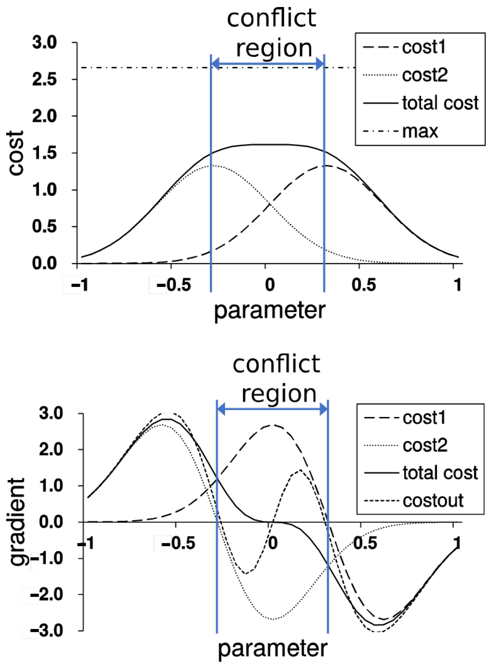
We posit gradient conflict between sub-costs as a cause of the accuracy limitation to learning the additive total cost. As shown in Figure 1-top, summing two distinct optimal values for each sub-cost shows a higher cost than the optimum for the total cost in a simple maximization problem. This degradation of summing sub-costs is due to gradient conflict shown in the Figure 1-bottom, which cancels each other and results in a zero gradient plateau at subpar optimum. Splitting the network into a completely separate model for each sub-cost is undesirable because it loses the benefits of using multiple sub-costs for training. The purpose of Cost-Out is to take advantage of multi-task learning and reduce accuracy limits.

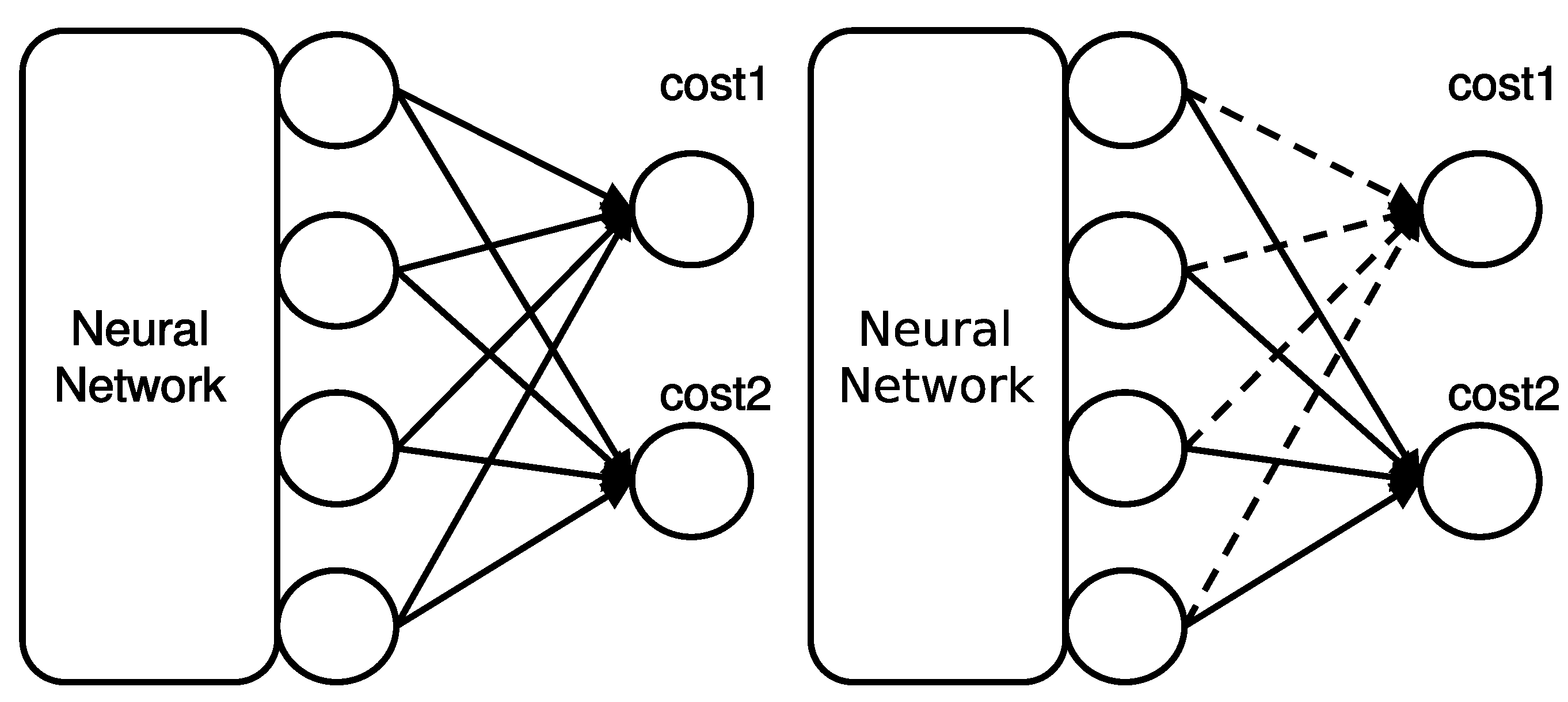
3.2. Method: Stochastic Switching of Sub-Costs

Unlike a typical multi-task learning scheme (see Figure 2-left), Cost-Out stochastically excludes a subset of sub-costs at each parameter update in the training phase, as illustrated in Figure 2-right. In this paper, we describe approaches of Cost-Out that attempt to incorporate “dropout” mechanism with two variants: a soft Cost-Out (sCO) and a hard Cost-Out (hCO). It is the same as dropout applied on the final layer if we apply this method with a given probability p for each sub-cost drop. However, adopting the original dropout mechanism for cost drop, which is a soft Cost-Out, is not suitable to cause escaping pressure since there is a chance of all sub-costs being selected for an update. If, then, the model again moves toward the optimum of the total cost. Therefore, we also adopt a method, updating only one sub-cost at a time, which is a hard Cost-Out.

3.3. Estimation of Escaping Pressure

Cost-Out derives the gradients using only the sampled sub-costs at every update. We can obtain a series of sub-costs by iterating updates, and we can observe several patterns by examining their gradients. It can be largely divided into two cases depending on the direction of the generated gradients. The first case is that a series of gradients repeat updates in a similar direction, which implies that local optima of a set of sub-costs exist in roughly the same location. In this case, repeating the probabilistic selection helps the movement to the optimum. The second case is that the gradients repeat the update in the opposite direction, resulting in conflicts between sub-costs near the local optimum of the total cost. In the latter case, Cost-Out leads to a drift effect by introducing additional non-zero gradients. We will show the existence of the drift and estimate their amount in the following derivation. We call the parameter range that causes cancellation as the conflict region.

Assume a simple case that the combined cost is the sum of two sub-cost $c_1$ and $c_2$. Then, $c_1$ is used for updating a value set ${\theta }_0$ for parameters of a neural network. ${\theta }_1$ indicates the changed parameter values after the update. The canceling case occurs when $c_2$ is selected near the local optimum of the combined cost. In this case, gradient $c_2$ at ${\theta }_1$ is

$$\begin{array}{c}\hfill {\nabla }_{{\theta }_1}^{c_2}={\nabla }_{{\theta }_0}^{c_2}+\lambda {\mathbf{H}}_{{\theta }_0}^{c_2}{\nabla }_{{\theta }_0}^{c_1},\end{array}$$

(1)

where $\lambda$ is a learning rate and ${\nabla }_{{\theta }_0}^{c_1}$ is the gradient calculated from the previous update step. ${\nabla }_{{\theta }_0}^{c_2}$ is the gradient and ${\mathbf{H}}_{{\theta }_0}^{c_2}$ is the main diagonal values of Hessian matrix of $c_2$ at ${\theta }_0$. Then, the result gradient ${\tau }_{c_1}$ of selecting $c_1$ and $c_2$ sequentially is derived as

$$\begin{array}{ccc}\hfill {\tau }_{c_1}& =& {\nabla }_{{\theta }_0}^{c_1}+{\nabla }_{{\theta }_1}^{c_2}\hfill \\ & =& {\nabla }_{{\theta }_0}^{c_1}+{\nabla }_{{\theta }_0}^{c_2}+\lambda {\mathbf{H}}_{{\theta }_0}^{c_2}{\nabla }_{{\theta }_0}^{c_1}\hfill \\ & =& {\nabla }_{{\theta }_0}^c+\lambda {\mathbf{H}}_{{\theta }_0}^{c_2}{\nabla }_{{\theta }_0}^{c_1}\hfill \end{array}$$

(2)

If the probabilities to select $c_1$ and $c_2$ are equal, expected gradient $\tau$ is

$$\begin{array}{ccc}\hfill \tau & =& \frac{1}{2}({\tau }_{c_1}+{\tau }_{c_2})\hfill \\ & =& {\nabla }_{{\theta }_0}^c+\frac{\lambda }{2}({\mathbf{H}}_{{\theta }_0}^{c_2}{\nabla }_{{\theta }_0}^{c_1}+{\mathbf{H}}_{{\theta }_0}^{c_1}{\nabla }_{{\theta }_0}^{c_2}).\hfill \end{array}$$

(3)

Here, we can confirm that the gradient of sequential canceling updates of Cost-Out is not equal to that of total cost c. If the network is near an optimum,

$$\begin{array}{c}\hfill {\nabla }_{{\theta }_0}^c={\nabla }_{{\theta }_0}^{c_1}+{\nabla }_{{\theta }_0}^{c_2}\sim 0.\end{array}$$

(4)

This relation converts the expected total gradient to

$$\begin{array}{ccc}\hfill \tau & \sim & \lambda ({\mathbf{H}}_{{\theta }_0}^{c_2}{\nabla }_{{\theta }_0}^{c_1}+{\mathbf{H}}_{{\theta }_0}^{c_1}{\nabla }_{{\theta }_0}^{c_2}).\hfill \end{array}$$

(5)

This result is drawn in the Figure 1 bottom for comparison with the original gradient of the combined cost.

The simple case can be generalized to complex cost functions by extending the results to a set of selected sub-costs $C_i$ and its complement $C_i^c$. The gradient ${\nabla }_{{\theta }_1}{C}_i$ at ${\theta }_1$ is

$$\begin{array}{c}\hfill {\nabla }_{{\theta }_1}{C}_i=\sum _{c\in C_i}{\nabla }_{{\theta }_0}c+\lambda \sum _{c\in C_i}{\mathbf{H}}_{{\theta }_0}^c\sum _{d\in {C_i}^c}{\nabla }_{{\theta }_0}^d\end{array}$$

(6)

and the gradient ${\tau }_{C_i}$ after an update with selected $C_i$ is

$$\begin{array}{ccc}\hfill {\tau }_{C_i}& =& {\nabla }_{{\theta }_0}C+\lambda \sum _{c\in C_i}{\mathbf{H}}_{{\theta }_0}^c\sum _{d\in {C_i}^c}{\nabla }_{{\theta }_0}^d.\hfill \end{array}$$

(7)

Then, we can derive the expected gradient $\tau$ overall possible combinations for $C_i$ whose sub-costs are selected by Bernoulli distribution with respect to p.

$$\begin{array}{ccc}& & \tau =\sum _{C_i}p\left(C_i\right){\tau }_{C_i}={\nabla }_{{\theta }_0}C+\lambda {\delta }_{{\theta }_0},\hfill \\ & & {\delta }_{{\theta }_0}=\sum _{C_i}{p}^{|C_i|}{(1-p)}^{N-|C_i|}\sum _{c\in C_i}{\mathbf{H}}_{{\theta }_0}^c\sum _{d\in {C_i}^c}{\nabla }_{{\theta }_0}^d\hfill \end{array}$$

(8)

The pressure ${\delta }_{{\theta }_0}$ can be simplified as follows:

$$\begin{array}{ccc}\hfill {\delta }_{{\theta }_0}& =& p(1-p)\sum _{(c,d)s.t.c\ne d}{\mathbf{H}}_{{\theta }_0}^c{\nabla }_{{\theta }_0}^d.\hfill \end{array}$$

(9)

As the result of this derivation, the escaping pressure is determined by $p(1-p)$, the amount of Hessian diagonal and gradient multiples for all combinations of two different sub-costs.

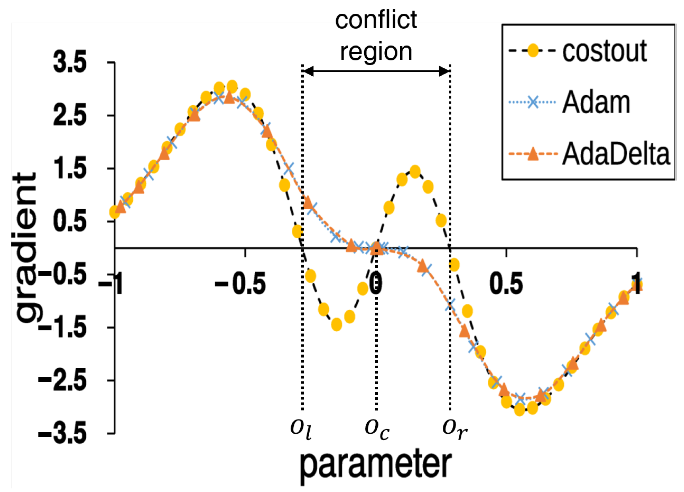
3.4. Convergence of Cost-Out Compared to Other Optimization Methods

To see the effect of the escaping pressure on optimization, we show the convergence simulation of SGD with the estimated escaping pressure in Figure 3. For comparison, we also plot the simulation of two popular momentum-based optimizers: Adam [23] and AdaDelta [24]. In the landscape, there are three optima: optimum at center $x=0$ ($o_c$), optima at left and right boundary of conflict region ($o_l$ and $o_r$, respectively). If the probability of sub-cost selection is assumed as even, the use of Cost-Out forces gradient-based stochastic optimizer to move toward the two candidate optima $o_l$ and $o_r$ with an equal chance. This causes stochastic perturbation since small movements by update within the conflict region diverge to the boundaries, as summarized in

Table 2. Convergence to optima in conflict region.

Gradient Sign
	Near ${\mathit{o}}_{\mathit{l}}$		Near ${\mathit{o}}_{\mathit{c}}$		Near ${\mathit{o}}_{\mathit{r}}$
	Left	Right	Left	Right	Left	Right
w/Cost-Out	+	-	-	+	+	-
w/o Cost-Out	+	+	+	-	-	-
Convergence to Optimum
w/Cost-Out	converge		diverge		converge
w/o Cost-Out	pass		converge		pass

.

By the effect of escaping pressure, the model parameters are updated repeatedly until they meet the regularities of two optima $o_l$ and $o_r$. This phenomenon is only observable when the optimization procedure is affected by the escaping pressure but not momentum (e.g., Adam, AdaDelta). Those momentum-based optimizers are designed to correctly find the optimum of the total cost rather than changing the cost landscape. While both dropout and Cost-Out induce escaping pressure, only Cost-Out reduces the gradient conflict between sub-costs since the original dropout applied to the internal layers only decreases the total cost via parameter update.

4. Experiments and Results

Cost-Out is a generic yet straightforward mechanism that drops gradients of partial tasks rather than simultaneously learning the entire gradients of every task. To verify the effectiveness of Cost-Out, we adopt two representative tasks in the field of vision and language—image classification and machine translation.

4.1. Classifying Two-Digit Images Sampled from the Same Set (TDC-Same)

The goal of this problem is to predict two digits with a neural network from a concatenated two $28\times 28$ input images of MNIST dataset [25]. Compared to separately classifying each digit from its corresponding image, this problem is more complex because of the interaction between features of two different images in a single network. The cost function is defined as below:

$$\begin{array}{cc}\hfill f_{\mathrm{sub}}(\mathbf{o},\mathbf{y})=& {\sum }_{i=1}^d{\left(\mathbf{y}\right)}_{i}ln\frac{e^{{\left(\mathbf{o}\right)}_i}}{{\sum }_j^d{e}^{{\left(\mathbf{o}\right)}_j}}\end{array}$$

(10)

$$\begin{array}{cc}\hfill f_{\mathrm{TDC}}\left(D\right)=& E\left[f_{\mathrm{sub}}({\mathbf{o}}_1,{\mathbf{y}}_1)+f_{\mathrm{sub}}({\mathbf{o}}_2,{\mathbf{y}}_2)\right],\end{array}$$

(11)

where d is the length of output vector o. The partial output vector ${\mathbf{o}}_1$ and ${\mathbf{o}}_2$ are generated from two input images. ${\mathbf{y}}_1$ and ${\mathbf{y}}_2$ are one-hot vectors to indicate correct digit label index. The data set D is composed of inputs generating ${\mathbf{o}}_1$ and ${\mathbf{o}}_2$, and corresponding ${\mathbf{y}}_1$ and ${\mathbf{y}}_2$. The $f_{\mathrm{TDC}}$ is the expectation of the two sub-costs over all data samples in D.

We use pre-split 50,000 training, 10,000 validation, and 10,000 test set as a publically released setting (http://www.iro.umontreal.ca/~lisa/deep/data/mnist/mnist.pkl.gz, accessed on 21 April 2021). Samples in each set are copied once, randomly shuffled, and then concatenated with the original set. Final data have the same sample size as the MNIST data, but each sample has twice a larger input dimension and output class size.

The impact of Cost-Out is likely to be affected by the other regularization techniques since it also has a regularization effect. For example, if regularization is too strong compared to the given model capacity, Cost-Out may decrease performance. To evaluate the performance of Cost-Out under this regularization-sensitive condition, we select combinations of typical regularization methods such as $L_2$ penalization, batch normalization (BN) [26], dropout, and model size changing. The detailed combination settings are shown in the

Table 3. Hyper-parameter settings for TDC-same task.

Hyper-Parameter	Value
Dropout Probability	$0.1,0.5,0.9$
Batch Normalization	decaying
· Decaying Rate	0.99 per epoch
$L_2$ scale	$0,{10}^{-5},5\times {10}^{-5},$
	${10}^{-4},5\times {10}^{-4},{10}^{-3}$
Cost-Out Type	soft, hard
Optimizer	SGD, Adam
· SGD Learning Rate	${10}^{-2},{10}^{-3}$
· Adam Learning Rate	${10}^{-4}$
· Adam (${\beta }_1$, ${\beta }_2$)	$(0.9,0.999)$
Hidden Layer Size	$512,2048$
Batch Size	32
Activation	tanh

.

BN is decayed by gradually reducing the interpolation rate between normalized and original activations. The optimal number of hidden nodes of the layers reported in the original MNIST challenge is near 800 [27], so we test one smaller model and the one larger model than the reported model. Model parameters are initialized by randomly selecting a real value in $[-\frac{1}{\sqrt{n}},\frac{1}{\sqrt{n}}]$ where n is the number of parameters of a layer [28].

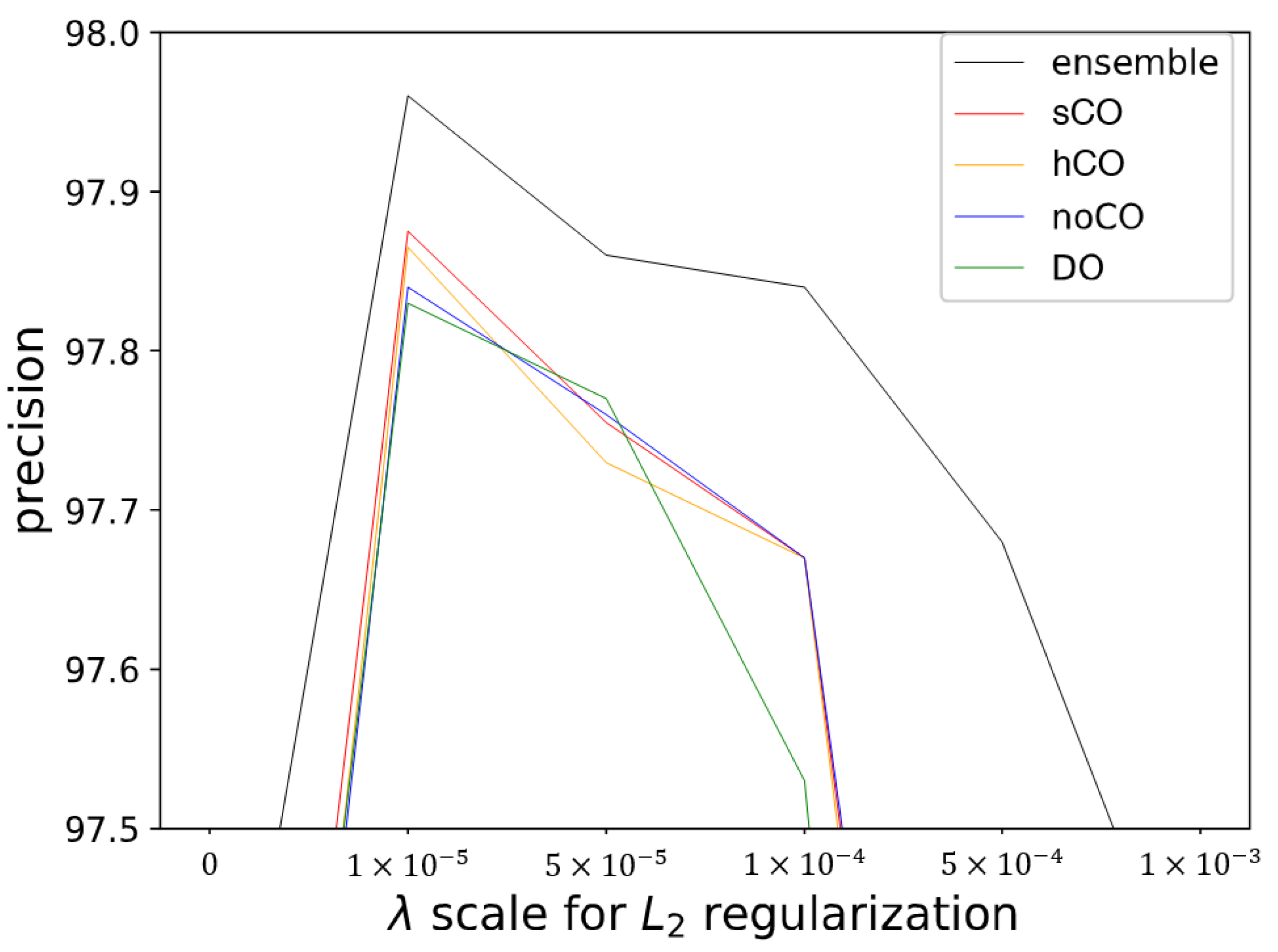
4.1.1. Performance Recovery under Various Regularization Effects

We plot the maximum performance of TDC-same in the Figure 4. This result is collected from various combinations of regularization methods and hyper-parameters. The optimal $L_2$ is ${10}^{-5}$ for all settings. The ensemble shows the best performance among the overall regularization settings. TDC-same problem has no advantage from resource sharing so that only the negative effect of gradient conflict occurs. Thus, the ensemble completely removes the conflict issue, and its result is the upper bound of the performance of multi-task learning. Both Cost-Out versions have improved performance compared to an ordinary case and even the case using dropout, which implies that the model averaging and regularization effects of dropout are orthogonal to the sub-cost switching.

In

Table 4. Best performance in the test set of TDC-same task. Common best configuration: Adam, no dropout, 2048 hidden nodes, ${10}^{-4}$$L_2$ scale (P.: precision, p: $\mathrm{recovery}\mathrm{rate}=\frac{\mathrm{error}\mathrm{by}\mathrm{multiple}\mathrm{sub}-\mathrm{costs}}{\mathrm{error}\mathrm{after}\mathrm{applying}\mathrm{Cost}-\mathrm{Out}}$).

Input	Output	Method	Best P.	p	BN
dual	single	ensemble	97.96	–	o
dual	dual	without Cost-Out	97.84	0.00	x
dual	dual	with hard Cost-Out	97.87	0.21	x
dual	dual	with soft Cost-Out	97.88	0.29	x

, detailed numerical results are shown. This ensemble result is higher than the case of not using Cost-Out by 0.12% at the best cases. Applying Cost-Out improves performance compared to the best result of not using the Cost-Out method by 0.04% precision, which is 29% recovery of the performance decrease by using multiple sub-costs. In the case of dropout, it seriously decreases the best performance in large $L_2$ scales, and its maximum was lower than the Cost-Out methods. This evaluation confirms that applying Cost-Out can recover the decreased best performance by using multiple sub-costs. In

Table 5. Detailed performance change by applying Cost-Out or dropout in TDC-same with various settings. (d: dimension of the hidden layer, y-axis: average precision, x-axis: scale of $L_2$ penalty).

d = 512	d = 2048	d = 512	d = 2048
SGD		Adam
SGD + batch norm		Adam + batch norm

, more detailed performance changes are plotted.

With stochastic gradient descent, the performance gain from Cost-Out is much more significant than the standard model. Regularization does not entirely explain this gain because the effect is consistently observed under various regularization strength—$L_2$ penalty scales and dropout. Even when using Adam, the gain is smaller, but the performance is not the same as in the typical case, which implies the effect of escaping pressure. When applying batch normalization, the gain in the SGD case almost disappears. In overall results, we can see that there is some evidence that escaping pressure affects the performance, but it can be easily hidden by batch normalization or optimizer.

4.1.2. Relaxation of Gradient Conflict

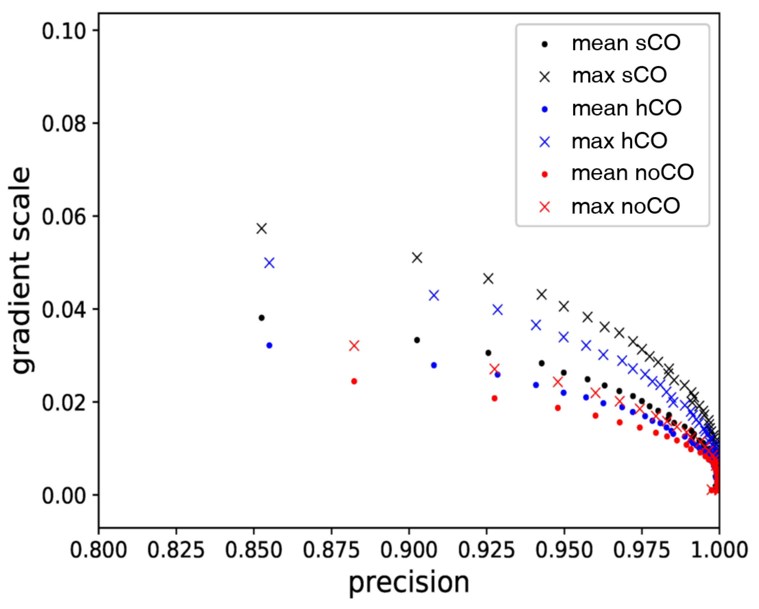
To investigate the impact of Cost-Out on optimization, we investigate the mean and max absolute values of all gradient elements with respect to the total cost, called gradient scale, in this section. This metric represents the steepness near the optima in the convex rather than the gradient values for various sub-cost combinations.

In Figure 5, we see that Cost-Out vastly increases gradient scale. This phenomenon supports that adopting Cost-Out causes escaping pressure. When applying Cost-Out, the gradient scale with respect to the total cost is the sum of the values in convex landscapes of its sub-costs, which is not affected by the gradient canceling. Therefore, applying Cost-Out can increase the gradient scale by the canceled amount, consistent with the result.

4.2. Classifying Two-Digit Images Sampled from the Two Disjoint Sets (TDC-Disjoint)

In TDC-same task, parameters of all layers except the final fully-connected layer are shared with all sub-costs. Therefore, the optima for two sub-costs using the copied data may be similar, even if not the same, by random initialization on the final layer. To prepare a more practical environment generating different optima for sub-costs, we set a new problem TDC-disjoint using two different disjoint image sets for 0 to 4 and 5 to 9 of MNIST data. Cost is calculated as the Equation (10), but the used data set D is composed of concatenated vectors of two disjoint sets. Training, validation, and test sample sizes are half of the TDC-same task. Practical networks are usually very deep, so we focus on evaluating the effect change by the depth increase. In this experiment, we use batch normalization with decaying, Adam optimizer with learning rate 1 × 10${}^{-4}$, 2000 hidden nodes per layer, tanh activation, hard Cost-Out, and no penalization. In the setting, we vary the number of layers from 1 to 10.

Performance Change by Deep Structuring

The impact of the escaping pressure is amplified by increasing the number of layers. Figure 6 shows the best precision in training data averaged over a total of five runs. There is no difference between using Cost-Out and not using it in the first to fifth layers, but using Cost-Out shows better results from the sixth layers. However, neither model found the optimum when they reached a depth of 9 to 10.

4.3. Machine Translation with Hierarchical Softmax (MT-Hsoftmax)

For machine translation tasks with hierarchical softmax, we combine two data sets, Europarl-v7 and CommonCrawl data provided from WMT 2014 (http://www.statmt.org/wmt14/, accessed on 21 April 2021). Tokenizing, lower-casing and cutting off with 40 tokens are applied via tools provided by MOSES [29] (http://www.statmt.org/moses/, accessed on 21 April 2021). We have set up six tasks from French, Spanish, and German to English translation and vice versa. Each training set has 1.5 million sentence pairs and its 10% is used as a validation set. The test sets are the Newstest set consisting of 3000 sentences and the News-Commentary set consisting of 150,000 sentences. To set sufficient model capacity, we use four stacks of 1000 LSTM cells for the encoder and the same size for a decoder. Word vectors are explicitly trained by word2vec [30] and imported in training and translation phases (https://code.google.com/archive/p/word2vec/, accessed on 21 April 2021). Detailed model parameters are shown in

Table 6. Hyper-parameter settings for machine translation tasks.

Hyper-Parameter		Parameter Size
LSTM Stacks	4	Encoder	3.05 M
Cells per Stacks	1000	Decoder	3.10 M
dim. of Word	50	Output	11 M
dim. of Attention	250	Interface	0.19 M
Batch Size	128

.

We use a bidirectional recurrent neural network with global attention [31,32]. BN is applied to all net values for gate and cell vectors. The weight of normalization is decayed and converged to near 0 after about 20 epochs. Cost-Out is applied only in the training phase. We use Adam optimizer, which showed better results than SGD and AdaDelta in preliminary experiments.

To create a simple combined cost, we design a k-expansion softmax function defined as follows:

$$\begin{array}{cc}\hfill f_{\mathrm{MT}-\mathrm{hsoftmax}}\left(D\right)=& E\left[{\sum }_{i=0}^{K-1}{f}_{\mathrm{sub}}({\left(\mathbf{o}\right)}_{ki}^{k(i+1)},{\left({\mathbf{y}}_k\right)}_i)\right]\end{array}$$

(12)

where $\mathbf{y}$ is a one-hot vector to indicate a correct class index y and ${\mathbf{y}}_k$ is the k-expansion of y. The constant K is the number of sub-tasks equal to $\lceil {log}_{k}y\rceil$. The vector ${\left(\mathbf{o}\right)}_i^j$ is the segment of $\mathbf{o}$ from the i-th to the $(j-1)$-th element. Thus, each segment of the output vector represents the probability of selecting a correct class index at each position in the k-expansion of y. In our experiments, we set k as 1024 and the length K as 2 to cover vocabulary size more than one million.

Effect of Cost-Out in MT-hsoftmax

In MT-hsoftmax task, we validate the benefits of using Cost-Out by predicting a correct word and position of the target sentences with mean precision and BLEU metrics. The results are shown in the

Table 7. Performance change by using Cost-Out in MT-hsoftmax. ($CO$: Cost-Out, $S-T$: source-target, $P.$: precision, $B.$: BLEU, w and $w/o$: with and without Cost-Out, $\delta$: performance gain when using Cost-Out (score of w− score of $w/o$), $\mu \left(\delta \right)$: mean of $\delta$, $\sigma \left(\delta \right)$: standard deviation of $\delta$).

		Best Performance in Each Set						Performance of Selected Model
		Valid		Test1		Test2		Train	Test1		Test2
$\mathit{CO}$	$\mathit{S}-\mathit{T}$	$\mathit{P}.$	$\mathit{B}.$	$\mathit{P}.$	$\mathit{B}.$	$\mathit{P}.$	$\mathit{B}.$	$\mathit{P}.$	$\mathit{P}.$	$\mathit{B}.$	$\mathit{P}.$	$\mathit{B}.$
w	En-Fr	15.59	20.23	15.05	16.40	12.33	16.84	57.43	14.81	16.26	12.33	16.65
$w/o$		15.20	19.86	14.73	15.65	12.06	16.15	57.41	14.64	15.65	11.97	16.15
w	Fr-En	19.99	27.25	13.35	12.34	12.76	14.58	56.41	13.04	12.34	12.64	14.58
$w/o$		18.48	26.08	12.16	11.23	11.52	13.52	55.04	12.16	10.67	11.52	13.26
w	En-Es	16.07	16.50	14.75	13.38	14.50	16.27	48.84	14.75	12.37	14.50	15.05
$w/o$		16.14	16.24	14.71	13.33	14.81	16.23	47.03	14.71	12.43	14.76	14.80
w	Es-En	17.87	17.68	15.79	13.65	15.24	15.60	23.48	15.79	13.65	15.24	15.60
$w/o$		17.21	17.33	15.27	13.21	14.72	15.43	20.70	15.27	13.21	14.72	15.43
w	En-De	15.57	10.12	13.31	6.51	10.77	5.78	41.12	13.00	5.25	10.59	4.67
$w/o$		15.62	10.05	13.47	6.50	10.66	5.72	43.00	13.47	6.24	10.66	5.21
w	De-En	14.60	12.93	13.24	8.79	10.83	8.29	45.41	13.24	8.79	10.83	8.29
$w/o$		14.54	12.60	13.19	8.34	10.67	7.89	47.02	12.93	8.00	10.67	7.81
	$\mu \left(\delta \right)$	0.42	0.43	0.33	0.47	0.33	0.40	0.42	0.24	0.41	0.30	0.36
	$\sigma \left(\delta \right)$	0.61	0.38	0.49	0.42	0.52	0.40	1.90	0.46	0.89	0.49	0.60

. Since the achievable translation quality largely varies in translation tasks, we measure the performance change by applying Cost-Out. In the results, the performance gain ($\delta$) in mean precision and BLEU ($\delta$) are almost positive when using Cost-Out, implying that Cost-Out improves translation quality. While dropout is not recommended to use in NMT because of its high sensitivity [33], Cost-Out can improve the performance without largely destroying the trained internal information.

4.4. Machine Translation Summing Costs of All Target Words (MT-Sum)

In Neural Machine Translation, summing cross-entropy values for classifying each word in the target sentence is a common approach which is also regarded as multi-task learning approach. To evaluate the impact of the escaping pressure, we set all the environment same as the MT-hsoftmax configuration except using hierarchical softmax. The cost function is defined as follows:

$$\begin{array}{cc}\hfill f_{\mathrm{MT}-\mathrm{sum}}\left(D\right)=& E\left[{\sum }_{i=0}^L{f}_{\mathrm{sub}}({\mathbf{o}}_i,{\mathbf{y}}_i)\right],\end{array}$$

(13)

where L is the length of tokens of a target sentence. Hard Cost-Out is applied to turn on and off of randomly selected half of the total words in a sentence.

Effect of Cost-Out in MT-Sum

The results of MT-sum task are shown in the

Table 8. Performance change by using Cost-Out in MT-sum.

		Best Performance in Each Set						Performance of Selected Model
		Valid		Test1		Test2		Train	Test1		Test2
$\mathit{CO}$	$\mathit{S}-\mathit{T}$	$\mathit{P}.$	$\mathit{B}.$	$\mathit{P}.$	$\mathit{B}.$	$\mathit{P}.$	$\mathit{B}.$	$\mathit{P}.$	$\mathit{P}.$	$\mathit{B}.$	$\mathit{P}.$	$\mathit{B}.$
w	En-Fr	19.43	26.60	18.92	22.52	15.73	22.88	65.30	18.59	22.28	15.51	22.77
$w/o$		20.48	31.74	13.99	15.69	13.72	18.77	68.46	13.99	15.69	13.61	18.77
w	Fr-En	21.45	32.11	14.15	15.54	13.92	18.98	70.41	14.15	15.54	13.92	18.98
$w/o$		20.21	31.44	13.27	15.08	13.36	18.64	69.94	13.22	15.05	13.36	18.64
w	En-Es	19.98	23.24	17.35	19.87	18.77	24.77	59.50	17.31	19.87	18.77	24.77
$w/o$		19.71	22.73	17.20	19.48	18.53	24.49	57.37	17.07	19.26	18.53	24.49
w	Es-En	21.95	24.62	18.76	19.52	19.66	24.24	59.36	18.53	19.27	19.66	24.24
$w/o$		21.73	24.67	18.38	19.73	19.45	24.29	59.69	18.21	19.5	19.45	24.29
w	En-De	18.28	14.47	15.46	10.46	12.52	9.54	51.18	15.26	10.39	12.51	9.40
$w/o$		18.24	14.52	15.60	10.65	13.01	10.09	48.96	15.40	10.65	12.58	9.45
w	De-En	17.30	17.74	15.53	13.63	13.27	13.29	50.07	15.39	13.48	13.27	13.29
$w/o$		16.96	17.38	15.28	13.30	12.85	12.75	49.22	14.98	13.13	12.70	12.56
	$\mu \left(\delta \right)$	0.18	−0.62	1.08	1.27	0.49	0.78	0.36	1.06	1.26	0.57	0.88
	$\sigma \left(\delta \right)$	0.73	2.24	1.92	2.74	0.83	1.68	1.99	1.77	2.64	0.70	1.56

. As with the previous results, we can see the effectiveness of Cost-Out by comparing the with and without Cost-Out. Although some of the results showed rather poor performance, they generally achieved positive performance gain. Through two experiments, MT-hsoftmax and MT-sum, we empirically demonstrate that applying Cost-Out when learning multiple sub-costs can bring the effect of finding a better optimum regardless of the sub-cost setting.

5. Discussion

We believe the main reason for the improved test performance in overall experiments is the escaping pressure induced by the Cost-Out mechanism (see Table 4, Table 7 and Table 8). Another possible reason for performance improvement may be due to other regularization methods. To find the setting that has little interference from regularization as possible and to verify the consistent effectiveness of Cost-Out in a various environment (i.e., different hyperparameter settings), we perform a grid search of hyperparameters, including batch normalization, drop-out, $L_2$-regularization, model capacity (i.e., dimension of the hidden layer), and gradient-based optimization methods (e.g., SGD, Adam) (see Figure 4, Table 5). Although using both Cost-Out and regularization can affect performance, using Cost-Out achieved the best results under most settings, implying that Cost-Out can generate orthogonal effects to the other regularization methods—we see this as an escaping pressure. Moreover, the plateau in the cost landscape, where the escaping pressure can improve the performance, is also observed in the results of gradient scale evaluation (see Figure 5). The change of gradient scale after applying for Cost-Out shows that the model converges to an optimum whose surrounding area has a steeper landscape. This observation supports that (1) the sum of training sub-costs for multitask learning can flatten optima and (2) Cost-Out causes escaping pressure to move the converging point to the boundary of the flattened area.

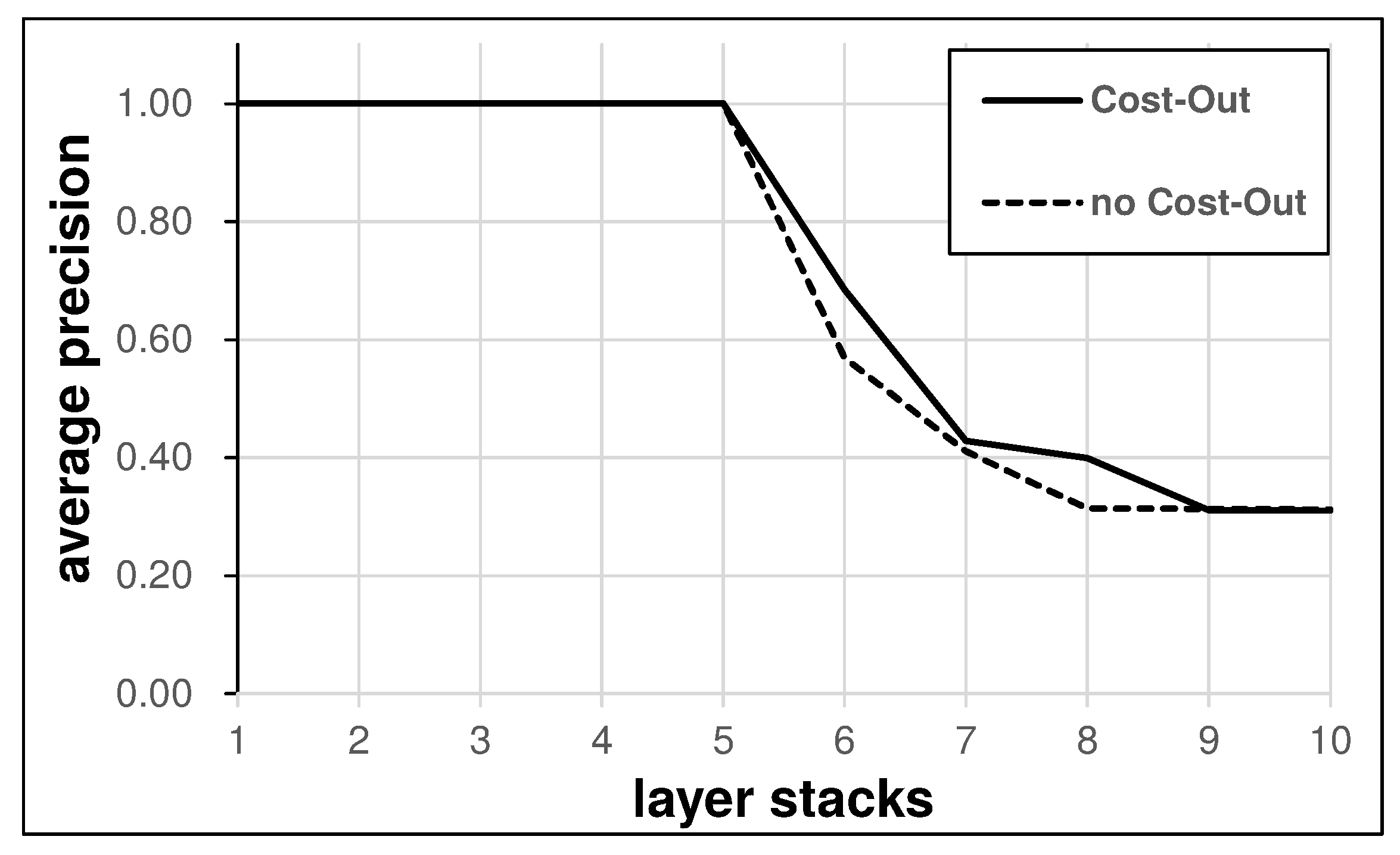
This escaping effect helps training in deep structures. As in Figure 6, stacking neural network layers gradually decreases training accuracy by gradient vanishing and probably landscape flattening by using more model parameters. Applying Cost-Out to this model improves the precision when the precision suffers from the negative effects by scaling up the model.

We conduct two experiments in different domains—vision and language—to show that the proposed methodology is domain- and structure-agnostic. We believe that it is not limited to these two tasks and can apply to more diverse multi-task learning problems since the approach itself can be applied if the total cost is defined as the summation of sub-costs.

6. Conclusions and Future Work

In this paper, we address the gradient conflict problem that arises during multi-task learning of neural networks. We postulate that this common problem in optimizing parameterized models can be solved with the escaping pressure induced in neural networks by applying Cost-Out, a dropout-like random selection mechanism. In the experiments, we empirically confirm the existence of escaping pressure that automatically selects gradients responsible for each task and forces them to learn the optimums for each sub-cost and its impact on two-digit image classifications and machine translation. Finally, we observe from the results that deep structured and insufficiently regularized models improve performance when using Cost-Out.

This work can be extended to demonstrate the benefits of using mini-batch-based training since the random selection of mini-batch for each update is identical to selecting a sub-cost for each mini-batch.

References

- Caruana, R. Multitask Learning. Mach. Learn. 1997, 28, 41–75. [Google Scholar] [CrossRef]
- Sener, O.; Koltun, V. Multi-Task Learning As Multi-Objective Optimization. In Proceedings of the Advances in Neural Information Processing Systems (NeurIPS), Montreal, QC, Canada, 3–8 December 2018; pp. 527–538. [Google Scholar]
- Kokkinos, I. Ubernet: Training a Universal Convolutional Neural Network for Low-, Mid-, and High-Level Vision Using Diverse Datasets and Limited Memory. In Proceedings of the IEEE Conference on Computer Vision and Pattern Recognition (CVPR), Honolulu, HI, USA, 21–26 July 2017; pp. 6129–6138. [Google Scholar]
- Zamir, A.R.; Sax, A.; Shen, W.; Guibas, L.J.; Malik, J.; Savarese, S. Taskonomy: Disentangling Task Transfer Learning. In Proceedings of the IEEE Conference on Computer Vision and Pattern Recognition (CVPR), Salt Lake City, UT, USA, 18–23 June 2018; pp. 3712–3722. [Google Scholar]
- Liu, X.; He, P.; Chen, W.; Gao, J. Multi-Task Deep Neural Networks for Natural Language Understanding. arXiv 2019, arXiv:1901.11504. [Google Scholar]
- Clark, K.; Luong, M.T.; Khandelwal, U.; Manning, C.D.; Le, Q. BAM! Born-Again Multi-Task Networks for Natural Language Understanding. In Proceedings of the 57th Annual Meeting of the Association for Computational Linguistics (ACL), Florence, Italy, 28 July–2 August 2019; pp. 5931–5937. [Google Scholar]
- Lu, J.; Goswami, V.; Rohrbach, M.; Parikh, D.; Lee, S. 12-in-1: Multi-Task Vision and Language Representation Learning. In Proceedings of the IEEE Conference on Computer Vision and Pattern Recognition (CVPR), Seattle, WA, USA, 14–19 June 2020; pp. 10437–10446. [Google Scholar]
- Ren, S.; He, K.; Girshick, R.; Sun, J. Faster r-cnn: Towards real-time object detection with region proposal networks. In Proceedings of the Advances in Neural Information Processing Systems (NeurIPS), Montreal, QC, Canada, 7–12 December 2015; pp. 91–99. [Google Scholar]
- Redmon, J.; Divvala, S.; Girshick, R.; Farhadi, A. You Only Look Once: Unified, Real-Time Object Detection. In Proceedings of the IEEE Conference on Computer Vision and Pattern Recognition (CVPR), Las Vegas, NV, USA, 27–30 June 2016; pp. 779–788. [Google Scholar]
- Simonyan, K.; Zisserman, A. Very Deep Convolutional Networks for Large-Scale Image Recognition. arXiv 2014, arXiv:1409.1556. [Google Scholar]
- Mi, H.; Sankaran, B.; Wang, Z.; Ittycheriah, A. Coverage Embedding Models for Neural Machine Translation. In Proceedings of the 2016 Conference on Empirical Methods in Natural Language Processing, Austin, TX, USA, 1–4 November 2016; pp. 955–960. [Google Scholar]
- See, A.; Liu, P.J.; Manning, C.D. Get To The Point: Summarization with Pointer-Generator Networks. In Proceedings of the 55th Annual Meeting of the Association for Computational Linguistics (ACL) (Volume 1: Long Papers), Vancouver, BC, Canada, 30 July–4 August 2017; Volume 1, pp. 1073–1083. [Google Scholar]
- Mikolov, T.; Sutskever, I.; Chen, K.; Corrado, G.S.; Dean, J. Distributed representations of words and phrases and their compositionality. In Proceedings of the Advances in Neural Information Processing Systems (NeurIPS), Lake Tahoe, NV, USA, 5–8 December 2013; pp. 3111–3119. [Google Scholar]
- Baxter, J. A Model of Inductive Bias Learning. J. Artif. Intell. Res. 2000, 12, 149–198. [Google Scholar] [CrossRef]
- Fliege, J.; Svaiter, B.F. Steepest Descent Methods for Multicriteria Optimization. Math. Methods Oper. Res. 2000, 51, 479–494. [Google Scholar] [CrossRef]
- Kendall, A.; Gal, Y.; Cipolla, R. Multi-Task Learning Using Uncertainty to Weigh Losses for Scene Geometry and Semantics. In Proceedings of the IEEE Conference on Computer Vision and Pattern Recognition (CVPR), Salt Lake City, UT, USA, 18–23 June 2018; pp. 7482–7491. [Google Scholar]
- Srivastava, N.; Hinton, G.; Krizhevsky, A.; Sutskever, I.; Salakhutdinov, R. Dropout: A simple way to prevent neural networks from overfitting. J. Mach. Learn. Res. 2014, 15, 1929–1958. [Google Scholar]
- Hinton, G.E.; Srivastava, N.; Krizhevsky, A.; Sutskever, I.; Salakhutdinov, R.R. Improving neural networks by preventing co-adaptation of feature detectors. arXiv 2012, arXiv:1207.0580. [Google Scholar]
- Baldi, P.; Sadowski, P.J. Understanding dropout. In Proceedings of the Advances in Neural Information Processing Systems (NeurIPS), Lake Tahoe, NV, USA, 5–8 December 2013; pp. 2814–2822. [Google Scholar]
- Collobert, R.; Weston, J. A unified architecture for natural language processing: Deep neural networks with multitask learning. In Proceedings of the 25th International Conference on Machine Learning (ICML), Helsinki, Finland, 5–9 July 2008; pp. 160–167. [Google Scholar]
- Oda, Y.; Arthur, P.; Neubig, G.; Yoshino, K.; Nakamura, S. Neural Machine Translation via Binary Code Prediction. arXiv 2017, arXiv:1704.06918. [Google Scholar]
- Sivaram, G.S.; Hermansky, H. Sparse multilayer perceptron for phoneme recognition. IEEE Trans. Audio Speech Lang. Process. 2012, 20, 23–29. [Google Scholar] [CrossRef]
- Kingma, D.P.; Ba, J. Adam: A method for stochastic optimization. arXiv 2014, arXiv:1412.6980. [Google Scholar]
- Zeiler, M.D. ADADELTA: An adaptive learning rate method. arXiv 2012, arXiv:1212.5701. [Google Scholar]
- LeCun, Y.; Bottou, L.; Bengio, Y.; Haffner, P. Gradient-based learning applied to document recognition. Proc. IEEE 1998, 86, 2278–2324. [Google Scholar] [CrossRef]
- Ioffe, S.; Szegedy, C. Batch normalization: Accelerating deep network training by reducing internal covariate shift. In Proceedings of the International Conference on Machine Learning, Lille, France, 6–11 July 2015; pp. 448–456. [Google Scholar]
- Simard, P.Y.; Steinkraus, D.; Platt, J.C. Best practices for convolutional neural networks applied to visual document analysis. In Proceedings of the Seventh International Conference on Document Analysis and Recognition (ICDAR), Edinburgh, UK, 6 August 2003; p. 958. [Google Scholar]
- Glorot, X.; Bengio, Y. Understanding the difficulty of training deep feedforward neural networks. In Proceedings of the Thirteenth International Conference on Artificial Intelligence and Statistics, Sardinia, Italy, 13–15 May 2010; pp. 249–256. [Google Scholar]
- Koehn, P.; Hoang, H.; Birch, A.; Callison-Burch, C.; Federico, M.; Bertoldi, N.; Cowan, B.; Shen, W.; Moran, C.; Zens, R.; et al. Moses: Open source toolkit for statistical machine translation. In Proceedings of the 45th Annual Meeting of the ACL on Interactive Poster and Demonstration Sessions, Prague, Czech Republic, 23–30 June 2007; pp. 177–180. [Google Scholar]
- Mikolov, T.; Chen, K.; Corrado, G.; Dean, J. Efficient estimation of word representations in vector space. arXiv 2013, arXiv:1301.3781. [Google Scholar]
- Bahdanau, D.; Cho, K.; Bengio, Y. Neural machine translation by jointly learning to align and translate. arXiv 2014, arXiv:1409.0473. [Google Scholar]
- Luong, M.T.; Pham, H.; Manning, C.D. Effective approaches to attention-based neural machine translation. arXiv 2015, arXiv:1508.04025. [Google Scholar]
- Zaremba, W.; Sutskever, I.; Vinyals, O. Recurrent neural network regularization. arXiv 2014, arXiv:1409.2329. [Google Scholar]
Figure 1.
Cost landscape for combined and decomposed costs. (
top) gradient conflict in cost perspective. (
bottom) gradient conflict in gradient perspective. (cost1: a normal distribution
, cost2:
, total cost: sum of cost1 and cost2, max: sum of optima of cost1 and cost2, costout: the expected gradient calculated in Equation (
3)).
Figure 2.
A schematic illustration of the Cost-Out mechanism. (left) Typical multi-task learning scheme learns all sub-costs per each update. (right) Cost-Out randomly drops the sub-costs with a given probability and learns only the remaining sub-costs per each update. The dotted line and solid line indicates dropped sub-cost and remaining sub-cost respectively.
Figure 3.
Comparison of convergence patterns between SGD + Cost-Out and other optimization methods. While there is only one optimum for Adam and AdaDelta, three possible optima exist for Cost-Out (i.e., gradient = 0): left (), center (), and right ().
Figure 4.
Achievable best performance of Cost-Out under regularization and batch normalization. (sCO: soft Cost-Out, hCO: hard Cost-Out, DO: dropout, noCO: without Cost-Out).
Figure 5.
The change in precision-gradient scale in the training phase of the TDC-same task. (sCO: soft Cost-Out, hCO: hard Cost-Out, noCO: without Cost-Out).
Figure 6.
Best precision averaged over five models by the number of stacked layers with or without Cost-Out in TDC-disjoint task.