HEVC Fast Intra-Mode Selection Using World War II Technique

Abstract

High-Efficiency Video Coding (HEVC) applies 35 intra modes to every block of a frame and selects the mode that gives the best prediction. This brute-force nature of HEVC makes it complex and unfit for real-time applications. Therefore, a fast intra-mode estimation algorithm is presented here based on the classic World War II (WW2) technique known as the ‘German Tanks Problem’ (GTP). This not only is the first article to use GTP for early estimation of intra mode, but also expedites the estimation process of GTP. Secondly, the various elements of the intra process are efficiently mapped to the elements of GTP estimation. Finally, the two variations of GPT are modeled and are also minimum-variance estimates. These experimental results indicate that proposed GTP-based fast estimation reduced the compression time of HEVC from 23.88% to 31.44%.

1. Introduction

The timely availability of multimedia content to a user is as important as the availability of intelligence in a war. In digital marketing, video covers 80% [1] of material. According to Cisco [2], 82% of total Internet traffic is videos. Moreover, a single HD television that is connected to the Internet will generate, on average, an equivalent amount of traffic to that generated by an entire family. This problem escalates when it comes to Ultra-High-Definition (UHD) devices, as they require double the HD video bit-rate. Cisco estimates that by 2023, 66% of televisions will be UHD. Therefore, an efficient algorithm is required that can reduce the size of multimedia content. Compression algorithms reduce the size of videos but maintain the same subjective video quality.

For this work, we will use the High-Efficiency Video Coding (HEVC) [3] compression standard. This standard, also known as H.265, reduces the bit-rate requirement by 50% and delivers the same subjective quality [4]. This bit-rate reduction is achieved by using big block sizes to compress smooth regions of the video, and small block sizes to compress textured regions. Moreover, the content of each block is predicted by using neighboring pixels. These neighboring pixels are projected onto the area of the current block in 35 different ways to achieve best prediction. These 35 projections are known as intra modes in HEVC.

HEVC can efficiently compress UHD content, and all issues related to UHD can be solved, but HEVC is not applicable to real-time applications. The complexity of HEVC has increased as compared to its previous standard, H.264. The complexity of HEVC increases as it tries all the block sizes and intra modes to predict the best tradeoff between rate and distortion, known as the RD cost. HEVC test model software, HM [5], first partitions the image into $64\times 64$-size blocks known as Coding Units (CUs) and the best intra mode is selected by applying all 35 intra modes. Then, this $64\times 64$ CU is partitioned into 4 CUs of equal size, and the same intra mode procedure is repeated on them. This CU partitioning and intra-mode selection process is repeated until the CU size reaches 8, which is the smallest CU in HEVC. This brute-force characteristic of HEVC makes it unfit for real-time application.

To reduce the complexity of HEVC, a fast intra-mode [6] decision-making task will be carried out in this article. There are 35 intra modes, and one of them is the best; therefore, a mechanism is needed that facilitates early intra-mode decision. Out of these 35 modes, 33 are angular modes that project neighboring pixels in 33 different ways onto the current CU. The remaining two modes are used to predict the smooth regions present in the image. Figure 1 [7] shows the directions of the 33 angular modes. The RMD module of the HM software shortlists up to 8 intra modes for the current block by using the Hadamard cost. The number of intra modes depends on the size of the block. The RMD module shortlists {8, 8, 3, 3, 3} intra modes for block size ∈ {$4\times 4$, $8\times 8$, $16\times 16$, $32\times 32$, $64\times 64$}, respectively. Then, the RDO module of the HEVC computes the RD cost for these intra modes (shortlisted by RMD) and selects 1 intra mode.

The proposed work is inspired by Optimal Stopping Theory (OST) and Classical Secretary Problem (CSP)-based models, and applied the German Tanks Problem (GTP) [8] algorithm to perform a fast intra-mode decision. The GTP algorithm is a statistical model just like OST and CSP, but is based on a true story. The GTP was created during World War II (WW2) to predict the number of tanks that the Germans had. This algorithm, GTP, not only predicted the number of tanks with great accuracy, but also discarded the claims made by intelligence. This victory over British and American intelligence gave GTP unique importance and significance. Moreover, the formulation of GTP is very simple. Therefore, this article applies GTP to predict the intra mode for the current CU. The proposed GTP-based algorithm outperformed existing algorithms. The main contributions of proposed algorithm include:

(i)

Being the first algorithm to use GTP for early intra-mode decisions.

(ii)

Having not only a strong foundation, but also computational efficiency.

(iii)

Providing a satisfactory tradeoff between rate and distortion, and performing better than many existing algorithms.

This article is structured as follows: related works, motivation, the proposed model, and results are presented in Section 2, Section 3, Section 4 and Section 5, respectively. After that, the article is concluded in Section 6.

2. Related Works

The literature is full of fast algorithms. One reason for intra-mode popularity is that it is a very challenging area because one mode must be selected from 35 modes. Therefore, the probability of selecting the correct option is only 0.02%.

In [9], 30% of the encoding time is saved by a classical secretary problem-based algorithm. This work evaluates a minimum of two modes to compute the stopping point. In [10], the pixel values of the left and above block are used to decide the planar mode. This results in a 14% time reduction in the encoding process. Zhu et al. in [11] saved 16.1% of the encoding time. In this work, the Hadamard transform is used instead of DCT.

The author of [12] saved 28% of the time by proposing a model that performs intra-mode selection in an iterative process. In each iteration, a few intra modes are selected from the available pool (i.e., 35 modes). In [13], a 60% time-saving is achieved. This work tries a sub-set of modes. Ying in [14] saved 38% of the time by proposing a model that uses RD as a stopping point. Zhang in [15] saved 38% of the time by proposing a model that consisted of three phases. In [16], a model is proposed that uses the complexity of the block to form three groups. Yeh in [17] computes an RD cost using co-located information. Then, this RD cost is used to compute the stopping point.

In [18], the RDOQ module was customized. This work used the coefficients of the transform to predict RD cost. Around 63% of the time was saved in this work. Zhang in [19] performed intra prediction using the gradient of the block. In [20], Hu saved 55% of the time by proposing a regression-based algorithm. Tariq in [21] saved 35% of the time by proposing a model based on stopping theory.

In [22], Kuanar saved 45% of the time by proposing a model based on CNN. Huang in [23] performed optimization of intra modes. According to Huang, this model can be used for early decisions of CU and PU. The time-saving was around 66% on average. The author of [24] saved 58% of the time by proposing a model based on random forest. In [25], 52%of the time was saved. This work selected an angular mode for the block by using the output of the planar mode applied on the same block.

Tian in [26] saved 20.45% of the time. This work used a deviation among pixels of the block to find the intra mode for the block. In [27], Gwon saved 31.54% of the time by proposing a model that used a classifier. The Hadamard cost was used as a feature in this classifier. In [28], uncertainty-based model was proposed for fast intra-mode decision. The main contribution of this work was that it incorporates uncertainty of the real world into the algorithm. Therefore, it dynamically adjusts itself to various situations. In [29], Munagala enhanced the holoentropy of HEVC. As a result, the PSNR is approved compared to the original HEVC. Improvement to PSNR is directly related to improvement in the subjective quality of the content. Therefore, this algorithm gives a realistic experience to the user. Liu, in [30], proposed a method that accurately predicted features from video sequences. This method helped overcome stability and quantity issues of feature-matching techniques. More features mean more information and, hence, such an algorithm gives a more accurate prediction. However, more features mean more computation. Therefore, features should only be used that efficiently represent the original data. Bahce, in [31], proposed a 3D-SPECK method for the encoding of geometry videos. Jridi in [32,33] proposed an architecture for Discrete Cosine Transform (DCT) to reduce the complexity of HEVC. This work approximates DCT better than the existing architectures. Tariq, in [34,35,36,37], used statistical models to make early decisions about the intra mode.

The proposed work, in comparison to the state-of-the-art works presented above, computes the probability of each intra mode. These probabilities are then passed to the GTP algorithm to estimate the stopping point. Moreover, GTP is modified to perform early estimation by using only k options such that k ≤ N, where N is the total number of options.

3. Motivation

First, we present the ’German Tanks Problem’ (GTP) algorithm here; otherwise, it will be difficult to know the importance of GTP and why it is being selected to perform early intra-mode decision. Statistically, GTP has great importance because it is based on a true story. In World War II (WW2), the Allies wanted to know how many tanks the Germans had. Such information was of great importance because it could affect the outcome of the war. Therefore, the British and the Americans asked statistical intelligence to estimate the number of tanks the German had. The statisticians had one key piece of information, which was the serial numbers on the captured tanks. This was enough for statisticians to make an estimate of the total number of tanks that had been produced up to any given moment.

A point estimate in sample statistics is used to estimate a population. In this case, the statisticians were trying to estimate the maximum tank serial number based on the sample of tanks. Suppose we have a sample of serial numbers of tanks S as follows:

$$S=\{77,289,224,219,464,51,367\}$$

(1)

One can compute many types of sample statistics for this S. For example, one can find the mean, mean + 1SD (SD: Standard Deviation), mean + 2SD, max + min, etc. To find out which of these statistics is best, we must perform some simulations and the best of them will be centered at 500. Now we look at some statistics and plot them on the graph to see how they perform. Figure 2 presents graphs of well-known statistics. The blue line in these graphs represents the population obtained from the statistics and the gray bars are the samples (S) that we have. The first statistic is the mean, as shown in Figure 2a. Figure 2a shows that this statistic estimates half the population. In Figure 2b, the maximum is used and it predicts close to maximum only. Similarly, Figure 2c,d show the graphs of ‘2 times the mean + 1 standard deviation (SD)’ and ‘1 mean + 2 SD’, respectively. The correct number of tanks the German had was 500, and now we see how statisticians estimated this number.

$$WW2=\frac{(m-1)(k+1)}{k}$$

(2)

The statisticians used (2) in WW2 to estimate the population, where m is the maximum serial number and k is the total number of tanks captured. This estimate takes the population maximum and multiplies it by a number that is slightly greater than 1, i.e., (Sample Size +1)/Sample Size. The rest of the story of WW2 regarding GTP is that the statisticians at that time reported that the Germans had 529 tanks, but the standard intelligence estimate was 1400 tanks. After the war, the Allies captured the German production records, which showed that the true number of tanks produced was 545, almost exactly what the statisticians had calculated. The most famous form of (2) is obtained by simplifying it as follows:

$$\begin{array}{cc}\hfill WW2=& \frac{(mk+m-k-1)}{k}\hfill \\ \hfill =& m+\frac{m}{k}-1-\frac{1}{k}\hfill \\ \hfill \approx & m+\frac{m}{k}-1\hfill \end{array}$$

(3)

This is also known as minimum-variance unbiased estimator. The most important feature of this estimator is that it predicts a single value for a set of values, N. Now, we solve the same problem by applying the optimal stopping theory concept. The main task is to estimate the value as soon as possible, where the serial numbers are shown one at a time. Moreover, these serial numbers are sorted in ascending order. We slightly modified (3) into (4) and its output is given in

Table 1. Proposed Fast Estimation Results (example-1).

k	Serial No.	${\mathit{P}}_{\mathit{k}}$
1	1	2
2	2	3.5
3	3	5

.

$$\begin{array}{cc}\hfill P_k=& m+\frac{{\sum }_{i=1}^k{p}_i}{k}-1\hfill \\ \hfill \approx & m+\frac{{\sum }_{i=1}^k{p}_i}{k}\hfill \end{array}$$

(4)

In (4), k is the number of elements seen so far, m is the highest value (serial number) among the seen elements, $p_i$ is the sum of all the serial numbers of the k elements seen so far. The working of (4) is explained with the help of an example; suppose a person has 3 cars in total and they have serial numbers on them. Equation (4) is applied to this situation and the result is presented in Table 1. Let us compute the first row of Table 1. The first row of Table 1 shows that the decision maker has seen one car, so k = 1, m = 1 because the serial number on this car is the highest serial number observed so far, and $p_i$ = 1, as the sum of serial number of seen element(s) is one. Therefore, $P_k$ = 2 ( 1 + 1/1). Then we see another car (2nd row of Table 1) with serial number 2, hence, k = 2, m = 2, $p_i$ = 3 and $P_k$ = 3.5 (2 + 3/2). It is interesting to see that the number 3 is estimated after seeing only two elements.

Let us see another example of the proposed formulation by applying it to the data given in (1), and its results are shown in

Table 2. Proposed Fast Estimation on S (example-2).

k	S	Sum (S)	${\mathit{P}}_{\mathit{k}}$
1	51	51	102
2	77	128	141
3	219	347	335
4	224	571	367
5	289	860	461
6	367	1227	572
7	464	1691	706

. In Table 2, k is the number of elements, S is the serial number of the tank that is currently captured, $Sum\left(S\right)$ is the summation of serial numbers up to k, and $P_k$ is the output of the proposed fast estimation. It is interesting to note that the value 461 is achieved by the 5th element. It is not accurate, but it is the best possible estimate made by looking at the minimum number of elements.

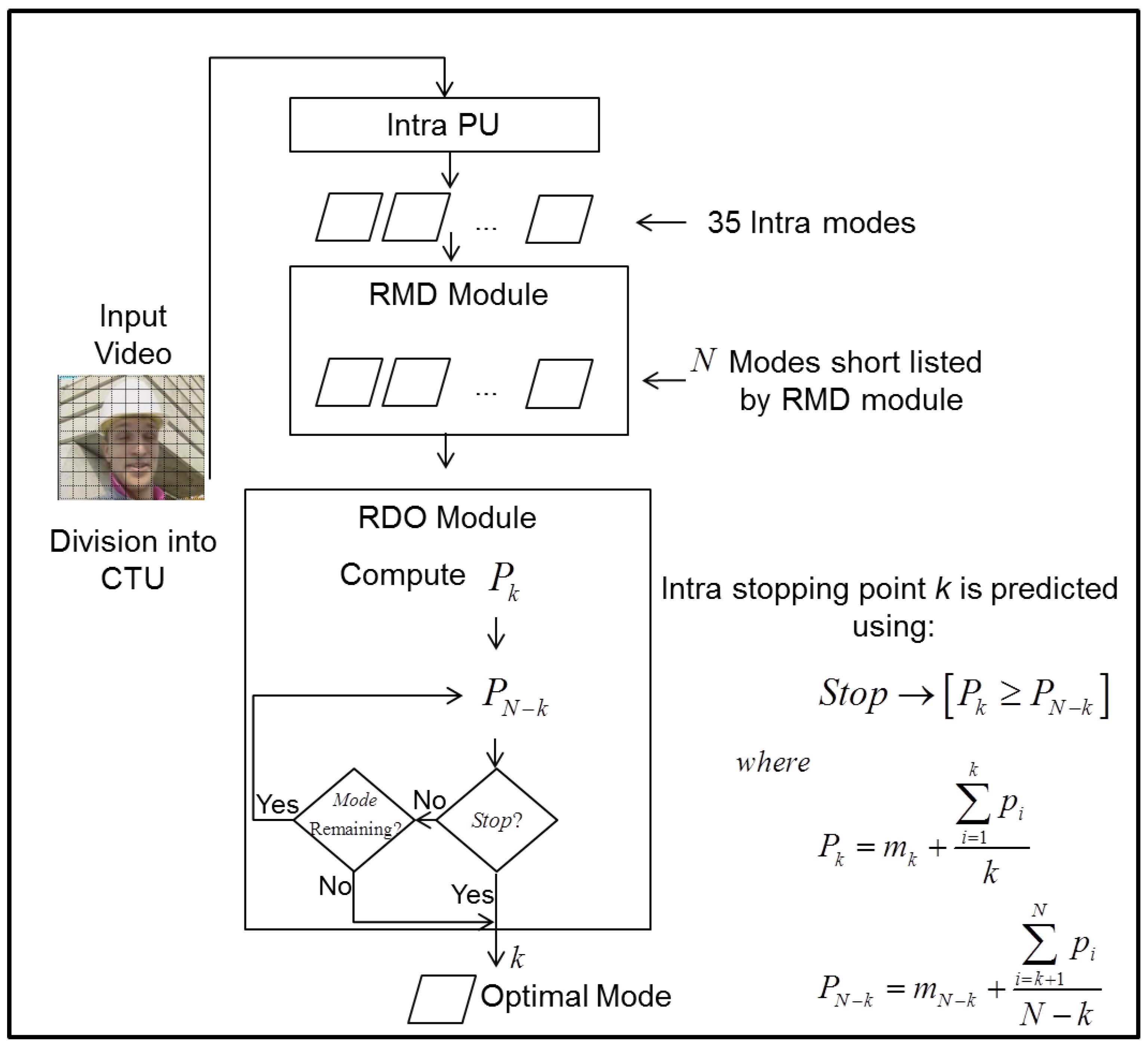
4. Proposed Algorithm

In this section, we will propose a fast intra-mode estimation technique using GTP. It is already shown in the previous section that it is possible to estimate an early value. Therefore, GTP concept will be extended in this section to estimate the intra mode early for the current CU.

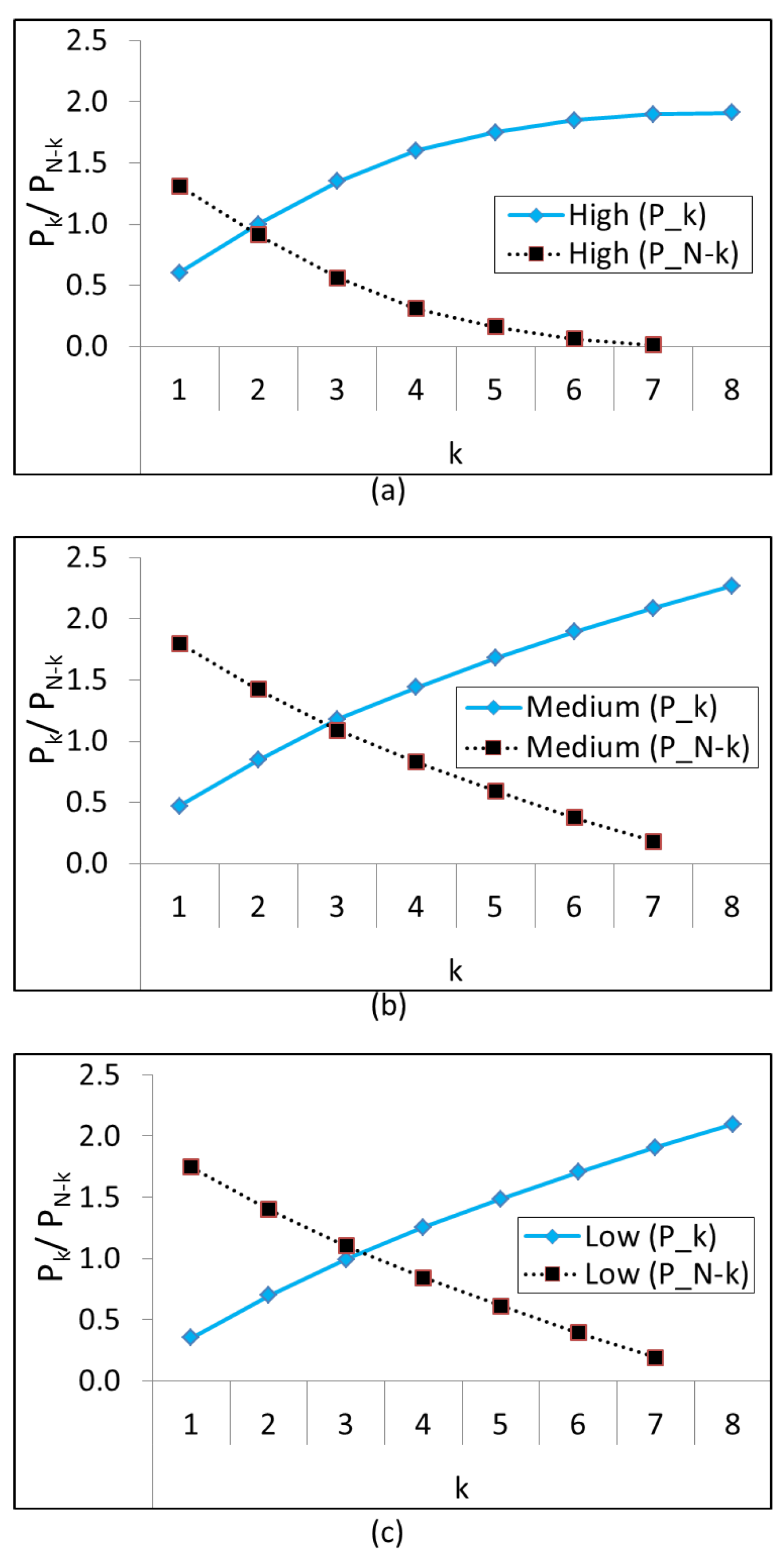
4.1. Hadamard Cost vs. Probability

The RMD module of HEVC shortlists N number of modes for the current CU by applying the Hadamard cost. Then, the RDO module performs operations on each of these N modes to obtain the RD (Rate Distortion) cost to find the optimal intra mode. The RDO module evaluates all these N modes, because it is possible that the RD cost of the first intra mode can be large and the RD cost of the Nth intra mode can be small. Therefore, we used the probabilities for the intra modes that are shortlisted by the RMD module. These probabilities are pre-computed and saved in a 2D matrix of size 35 × 35 because there are 35 modes. This matrix is shown in Figure 3. To obtain this matrix, we initialize this 2D matrix with zeros. Then we encode any video and when a mode is selected for the current block (e.g., j) and the neighboring mode is m, then we increment the value at mth column and jth row. This will give us the count matrix but it can be converted to probability by dividing it by the sum of all the values in this row j. After that, if the intra mode J is shortlisted by the RMD module for the current block, and by using this 2D matrix (given in Figure 3), we can compute its probability. The small spikes in Figure 3 mean that these modes have less probability to be selected, and big spikes in Figure 3 mean that these modes have high probability of selection. In this work, we obtained this matrix using a BasketballDrill video sequence because it contains fast and medium motion.

To construct a model and to perform simulations, three sets of values are selected from Figure 3 that are termed as ‘high’, ‘medium’, and ‘low’. The ‘high’, ‘medium’, and ‘low’ sets are obtained from different regions of this 2D matrix. The ‘high’ values are taken from a high peak region that indicates huge values, ‘medium’ values are taken from medium size peak and similarly, and ‘low’ values are taken from a flat region of a 2D matrix. The values in the ‘high’ set are: {0.30, 0.18, 0.12, 0.10, 0.08, 0.07, 0.06, 0.05 }; The values in the ‘medium’ set are: { 0.24, 0.17, 0.15, 0.10, 0.09, 0.08, 0.07, 0.06 }; The values in the ‘low’ set are: { 0.17, 0.17, 0.13, 0.11, 0.09, 0.09, 0.08, 0.07 }. The proposed early estimation, (4), is applied to these sets and their visual output is shown in Figure 4. In Figure 4, the values are decreasing because the ‘high’, ‘medium’ and ‘low’ sets are arranged in descending order. Figure 4 ‘high’ case gives higher values for early elements and gives very small values for the last elements. This indicates that the last elements have very little chance of being the optimal element. Where the ‘low’ case is concerned, the $P_k$ assigns values to the last elements such that they are greater than the ‘high’ case. This is a very interesting factor of the proposed model, assigning large values to the last elements of the ‘low’ case even though the values in the ‘low’ set are smaller than the values present in the ‘high’ case. The ‘low’ values do not descend very fast like the ‘high’ case because the probability is very low, and this indicates there is no clear information about the best element. Similarly, the ‘medium’ case in Figure 4 represents the intermediate case where the $P_k$ values for this case are lower than ’high’ but greater than ‘low’ values.

4.2. Trend of Proposed Early Estimator

The trend of $P_k$ for ‘high’, ‘medium’ and ‘low’ values are shown in Figure 5. Figure 5 shows that these values follow the natural-log trend ($ln$). The correlation coefficient (R) is also shown in Figure 5. This R is obtained using Microsoft Excel. Moreover, according to Wikipedia, GTP can also be written using a Bayesian formulation as follows:

$$N_{median}\approx m+\frac{mln\left(2\right)}{k-1}$$

(5)

Therefore, we can say that the proposed early estimation (i.e., (4)) is aligned with GTP, because it follows a natural-log ($ln$) trend.

4.3. Early Mode Decision Using Early Estimator

In HEVC, the first element given by the RMD module is selected 60% of the time, but there is no clue as to which are those 60% cases out of a total of 100%. That is why probabilities of these modes are used to extract some extra information about these modes that might help us make the early decision. Therefore, we need a stopping mechanism that performs early termination when these probabilities are high, and delay the early termination when these probabilities are low. Figure 5 clearly illustrates that the values are smooth and can be modeled using the natural log. Moreover, the drop in these values is also dependent upon the probabilities of these elements (see Figure 4), and this makes early estimation both dynamic and flexible. Therefore, an efficient early intra-mode decision can be performed using:

$$\begin{array}{cc}\hfill & P_k\ge P_{N-k}\hfill \\ \hfill where& \\ \hfill & P_k=m_k+\frac{{\sum }_{i=1}^k{p}_i}{k}\hfill \\ & P_{N-k}=m_{k+1}+\frac{{\sum }_{i=k+1}^N{p}_i}{N-k}\hfill \end{array}$$

(6)

This model evaluates elements from a sequential list one at a time and checks the above early-decision condition. At any element k, if $P_k$ becomes greater than the remaining elements, i.e., $P_{N-k}$, then this early termination is performed. It all depends upon the movement of k for different cases. For example, for ’high’ case, this k will be among the early elements of the list and for ’low’ case, this k will be among the later elements of the list.

The visual outputs of the proposed model (6) for three cases (‘high’, ‘medium’ and ‘low’) are shown in Figure 6. The movement of k is clearly visible for different cases. For ’high’ case, k has moved before the 2nd element and for ‘low’ case, this k has moved after the 3rd element, therefore making the model dynamic and flexible.

These examples show that the proposed algorithm handles various situations efficiently and dynamically, adjusting itself according to the elements. Moreover, the formulation of this early termination model is very simple and, as a result, it requires less computation.

The flowchart of the proposed algorithm is shown in Figure 7. The changes made to the RDO module are shown in the RDO box. For each CU, the RMD module evaluates 35 intra modes and shortlists up to N modes. Then, the proposed algorithm evaluates these intra modes given by the RMD module one by one until it finds the termination point, i.e., the point found using (6).

5. Experimental Results

Experimentation and comparison will be covered in this section. A slight change to the proposed model will be made to further improve the time-saving of the proposed model, but it will be presented in a separate table.

The proposed model is implemented in the recent HM version of HEVC i.e., 16.9. This HM software is downloadable from [5]. The HEVC dataset [38] contains various classes which include various videos. All these videos are coded using the "All Intra Main" configuration. This configuration is usually selected for intra-mode decision algorithms. In this configuration, all the CUs are intra-coded. Moreover, videos are encoded using 4 QPs (22, 27, 32, 37) to make comparison with the existing algorithms. The performance of the proposed algorithm is evaluated using BD-PSNR, time-saving, and BD-BR as recommended in [39]. Time-saving is computed using:

$$△T=\frac{\left(T_{HEVC\left(16.9\right)}-T_{PROPOSED}\right)}{T_{HEVC\left(16.9\right)}}\times 100\%$$

(7)

Experiments are conducted on a machine with 8 GB Ram, Intel i5 processor with computing power of 2.30 GHz and 64-bit operating system. First HM16.9 is executed to encode each test sequence five times and the mean of its time-saving is noted. Then, the proposed model is executed five times to encode the same sequences, and mean of time-saving is noted for comparison.

5.1. Encoding Results of Proposed Model

The compression results of the proposed model are presented in

Table 3. Result of proposed algorithm given in (6).

Classes	Video	$\Delta$P	$\Delta$R	$\Delta$T
A	Nebuta	−0.08	1.05	25.95
2560 × 1600	Traffic	−0.11	1.90	23.03
	PeopleOnStreet	−0.10	1.76	22.55
B	BQTerrace	−0.09	1.41	22.76
1920 × 1080	Cactus	−0.07	1.89	26.25
	Kimono	−0.10	2.88	25.61
C	BasketballDrill	−0.09	1.72	25.20
832 × 480	RaceHorses	−0.10	1.48	25.25
	PartyScene	−0.16	2.00	26.16
D	BlowingBubbles	−0.12	1.95	25.74
416 × 240	BQSquare	−0.17	1.94	26.25
	BasketballPass	−0.09	1.48	24.55
E	KristenAndSara	−0.10	1.96	23.48
1280 × 720	FourPeople	−0.12	2.06	21.45
	Johnny	−0.10	2.57	22.04
F	SlideShow	−0.23	0.99	23.12
1280 × 720	ChinaSpeed	−0.17	1.94	21.84
	BasketballDrillText	−0.07	1.37	23.10
Avg.		−0.11	1.79	24.13

. In Table 3, $\Delta$P, $\Delta$R and $\Delta$T stands for BD-PSNR, BD-BR, and time-saving, respectively. Table 3 shows that the proposed model saves 24% of the encoding time and costs 1.79% more bit-rate (BD-BR). The $\Delta$T column in Table 3 shows that there is some uniformity among the test video sequences. The maximum time-saving of the proposed model is 26.25 and the minimum time-saving is 21.45. Where BD-BR is concerned, the maximum BD-BR cost of the proposed model is 2.88 for the ‘Kimono’ test video and minimum BD-BR cost is 0.99 for the ‘SlideShow’ test video sequence.

To further improve the time-saving of the proposed model given in (6), its m term is removed to further reduce the complexity of the model. This resulted in a model given in (8).

$$\begin{array}{cc}\hfill & P_k^{\prime }\ge P_{N-k}^{\prime }\hfill \\ \hfill where& \\ \hfill & P_k^{\prime }=\frac{{\sum }_{i=1}^k{p}_i}{k}\hfill \\ & P_{N-k}^{\prime }=\frac{{\sum }_{i=k+1}^N{p}_i}{N-k}\hfill \end{array}$$

(8)

The encoding results of (8) are given in

Table 4. Result of proposed algorithm without term $m_k$ given in (8).

Classes	Video	$\Delta$P	$\Delta$R	$\Delta$T
A	Nebuta	−0.08	1.14	28.44
2560 × 1600	Traffic	−0.11	2.10	25.94
	PeopleOnStreet	−0.11	1.98	25.12
B	BQTerrace	−0.10	1.59	25.11
1920 × 1080	Cactus	−0.08	2.08	29.05
	Kimono	−0.10	2.80	27.71
C	BasketballDrill	−0.10	1.99	28.69
832 × 480	RaceHorses	−0.13	1.90	27.97
	PartyScene	−0.18	2.28	29.53
D	BlowingBubbles	−0.14	2.37	28.55
416 × 240	BQSquare	−0.18	2.09	31.44
	BasketballPass	−0.11	1.68	27.82
E	KristenAndSara	−0.11	2.12	25.04
1280 × 720	FourPeople	−0.13	2.21	23.88
	Johnny	−0.11	2.70	24.13
F	SlideShow	−0.19	0.85	25.35
1280 × 720	ChinaSpeed	−0.18	2.09	24.19
	BasketballDrillText	−0.08	1.50	25.85
Avg.		−0.12	1.97	26.88

. Table 4 shows that the time-saving is increased to 26.88%, and BD-BR increased to 1.97%. This is the maximum time-saving achieved with this model as we have tried two versions of GTP.

The comparison of both the variations of the proposed models is given in Figure 8. Figure 8 shows that if the time-saving is the need for the time, then one should prefer the model given in (8). Otherwise, one can use the model (6) to save the bit-rate overhead.

The subjective quality of the proposed algorithms is shown in Figure 9. By subjective, we mean the reconstruction quality of the video after compression. The reconstructions of the proposed models with and without $m_k$ terms are shown in Figure 9a,b, respectively. Figure 9 shows that there is not much subjective difference between the two variations. Even if we zoom the text present in the image, there is not much difference. Therefore, we can say that the overall quality of the proposed model(s) is satisfactory.

5.2. Proposed Model vs Existing Algorithms

To make a fair comparison with the existing algorithms, the proposed model is placed in

Table 5. Proposed Model vs Existing Algorithms.

Classes	Sequences	[41] (2020)			[42] (2020)			[43] (2019)			Proposed
		$\Delta$R	$\Delta$T	$\Delta$P	$\Delta$R	$\Delta$T	$\Delta$P	$\Delta$R	$\Delta$T	$\Delta$P	$\Delta$R	$\Delta$T	$\Delta$P
	Nebuta	-	-	-	-	-		-	-	-	1.14	28.44	−0.08
A	Traffic	-	-	-	0.69	22.89	−0.05	-	-	-	2.10	25.94	−0.11
2560×1600	PeopleOnStreet	-	-	-	0.81	24.31	−0.06	-	-	-	1.98	25.12	−0.11
	BQTerrace	0.10	22.03	−0.01	-	-	-	0.44	28.98	−0.02	1.59	25.11	−0.10
B	Cactus	0.10	10.52	0.00	-	-	-	0.54	28.05	−0.02	2.08	29.05	−0.08
1920×1080	Kimono	0.10	25.58	0.00	0.32	20.75	−0.01	0.35	18.70	−0.01	2.80	27.71	−0.10
	BasketballDrill	0.11	27.09	−0.01	1.04	23.73	−0.09	0.36	25.18	−0.02	1.99	28.69	−0.10
C	RaceHorses	0.08	27.24	−0.01	-	-	-	0.56	29.12	−0.04	1.90	27.97	−0.13
832×480	PartyScene	0.08	26.18	−0.01	-	-	-	0.50	30.81	−0.04	2.28	29.53	−0.18
	BlowingBubbles	0.13	10.11	−0.01	0.92	22.91	−0.09	0.70	30.60	−0.04	2.37	28.55	−0.14
D	BQSquare	0.10	8.02	−0.01	-	-	-	0.61	32.87	−0.05	2.09	31.44	−0.18
416×240	BasketballPass	0.01	10.34	0.00	0.77	23.66	−0.07	0.49	25.05	−0.03	1.68	27.82	−0.11
	KristenAndSara	0.10	11.93	0.00	-	-	-	0.59	24.56	−0.03	2.12	25.04	−0.11
E	FourPeople	0.13	8.87	−0.01	0.87	21.20	-0.06	0.66	25.59	−0.04	2.21	23.88	−0.13
1280×720	Johnny	0.11	9.51	0.00	0.78	20.49	−0.04	0.59	22.60	−0.02	2.70	24.13	−0.11
	SlideShow	0.01	15.50	0.00	-	-	-	0.66	25.12	−0.05	0.85	25.35	−0.19
F	ChinaSpeed	0.11	16.81	−0.01	-	-	-	0.83	27.85	−0.07	2.09	24.19	−0.18
1280×720	BasketballDrillText	0.10	8.73	−0.01	-	-	-	0.44	25.15	−0.02	1.50	25.85	−0.08
Average		0.09	15.90	−0.01	0.78	22.49	−0.06	0.55	26.75	−0.03	1.97	26.88	−0.12

along with three latest and state-of-the-art fast intra-mode decision algorithms. The term Proposed in Table 5 represents the proposed algorithm. The “-” in Table 5 means that the author of that algorithm did not mention the result of this test video sequence. Please note that some authors have reported huge time-saving, but that does not fall in fast intra mode decision as they combined fast CU, fast PU, and fast intra mode in a single algorithm. Moreover, the maximum possible time-saving achievable using intra mode decision is 40% [40]. The fast intra mode decision cannot be compared with a fast CU size decision because the intra mode decision is very different. The probability of selecting the right intra mode is only 0.02 (1/35). Hence, the intra-mode decision is very different and difficult.

Table 5 summarizes three pure intra-mode decision algorithms that include [41,42,43]. Moreover, their years of publication are also mentioned in parentheses “()”. The algorithm presented in [41] saves 15% of the time, [42] saves 22% of the time, and [43] saves 26.75% of the time. The proposed algorithm saves 26.88% of the time, which is very close to [43]’s time, but the methodology of the proposed work is unique, as this is the first article to employ GTP for fast intra-mode estimation. Moreover, the proposed algorithm is implemented in the latest HM version, i.e., 16.9, and each new version has some sort of optimization. Therefore, we can conclude that the proposed algorithm gives satisfactory results.

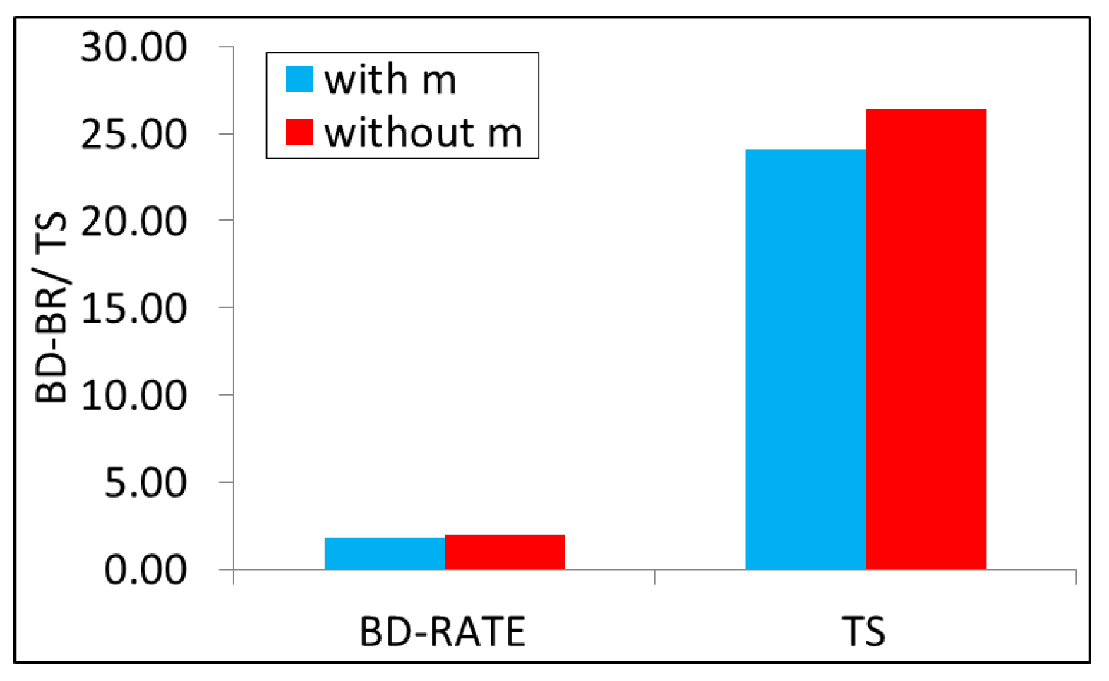
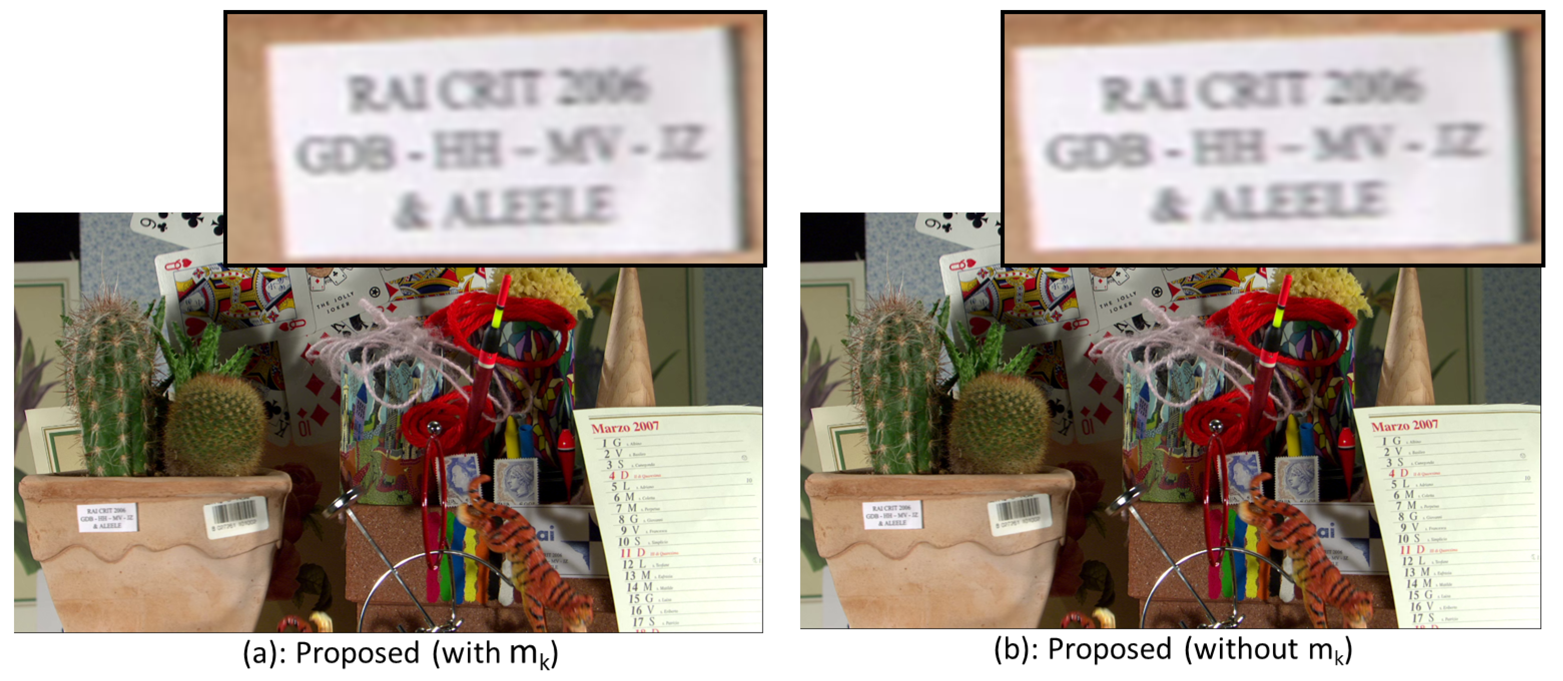
5.3. Analysis of Proposed Model

The proposed algorithm makes early terminations at different elements (intra modes) for different CUs. Sometimes, it will select the early element and sometimes it will select the latter element. The proposed model makes the early termination decision using (8) and if this condition is not successful then HEVC normal working continues. Therefore, the time consumed in decision-making will be the time consumed by (8). The time consumed by (8) for full search is $0.0010$ seconds on average.

Finally, we conducted an experiment that is presented in

Table 6. Fraction of modes skipped by proposed algorithm.

Sequences	QP				Average
	22	27	32	37
BlowingBubbles	48.98%	53.05%	56.42%	58.02%	54.12%
BQSquare	51.08%	55.77%	53.39%	50.53%	52.69%
BasketballPass	48.10%	51.38%	51.37%	47.21%	49.52%
Average	49.39%	53.40%	53.73%	51.92%	52.11%

. Table 6 shows that around 52.11% of the modes are skipped by the proposed algorithm. This percentage is obtained with the help of two variables; one variable (e.g., T) notes the number of modes shortlisted for the current block and another variable (e.g., S) records how many modes were remaining when early termination took place. Finally, the percentage is obtained by computing $S/T$. Table 6 presents this percentage for each QP, separately.

6. Conclusions

The intra mode for the current block is estimated using a classic technique of World War II (WW2). The German Tanks Problem (GTP) technique of WW2 was used to estimate the number of tanks the Germans had, and now it is applied to HEVC for intra-mode estimation due to its efficiency as well as accuracy. The proposed GTP-based fast intra-mode decision algorithm reduced the encoding time of HEVC from 23.88% (FourPeople) to 31.44% (BQSquare), with an average of 26.88%. Moreover, GTP is not only applied in the new area, i.e., estimation of intra mode, but also converted to fast estimation. The proposed estimation achieved the same goal, but its methodology is unique. It is worth mentioning that the proposed GTP-based algorithm outperformed the latest techniques [41,42,43] by saving 10.98%, 4.88%, and 0.13% more time, respectively.

References

1. Biteable. Available online: https://biteable.com/blog/video-marketing-statistics/ (accessed on 1 May 2020).
2. Biteable. Available online: https://www.cisco.com/c/en/us/solutions/collateral/executive-perspectives/annual-internet-report/white-paper-c11-741490.html (accessed on 1 February 2021).
3. Ugur, K.; Kenneth, A.; Arild, F.; Gisle, B.; Lars, P.E.; Jani, L.; Antti, H. High performance, low complexity video coding and the emerging HEVC standard. IEEE Trans. Circuits Syst. Video Technol. 2010, 20, 1688–1697. [Google Scholar] [CrossRef]
4. Ohm, J.R.; Gary, J.; Sullivan, H.S.; Thiow, K.T.; Thomas, W. Comparison of the coding efficiency of video coding standards including high efficiency video coding (HEVC). IEEE Trans. Circuits Syst. Video Technol. 2012, 22, 1669–1684. [Google Scholar] [CrossRef]
5. HEVC Test Model. Available online: https://hevc.hhi.frauhofer.de/svn/svn_HEVCSoftware/ (accessed on 1 August 2016).
6. Tariq, J.; Sam, K.; Hui, Y. HEVC intra mode selection based on rate distortion (RD) cost and sum of absolute difference (SAD). J. Vis. Commun. Image Represent. 2016, 35, 112–119. [Google Scholar] [CrossRef]
7. Zhang, M.; Zhai, X.; Liu, Z. Fast and adaptive mode decision and CU partition early termination algorithm for intra-prediction in HEVC. EURASIP Jo. Image Video Process. 2017, 1, 1–11. [Google Scholar] [CrossRef] [Green Version]
8. Ruggles, R.; Henry, B. An empirical approach to economic intelligence in World War II. J. Am. Stat. Assoc. 1947, 42, 72–91. [Google Scholar] [CrossRef]
9. Tariq, J. Intra mode selection using classical secretary problem (CSP) in high efficiency video coding (HEVC). Multimedia Tools Appl. 2019, 78, 31533–31555. [Google Scholar] [CrossRef]
10. Wang, L.-L.; Siu, W.-C. Novel adaptive algorithm for intra prediction with compromised modes skipping and signaling processes in HEVC. IEEE Trans. Circuits Syst. Video Technol. 2013, 23, 1686–1694. [Google Scholar] [CrossRef]
11. Zhu, J.; Liu, Z.; Wang, D.; Han, Q.; Song, Y. Fast prediction mode decision with Hadamard transform based rate-distortion cost estimation for HEVC intra coding. In Proceedings of the 2013 IEEE International Conference on Image Processing, Melbourne, VIC, Australia, 15–18 September 2013; pp. 1977–1981. [Google Scholar]
12. Zhao, L.; Zhang, L.; Ma, S.; Zhao, D. Fast mode decision algorithm for intra prediction in HEVC. In Proceedings of the Visual Communications and Image Processing (VCIP), Tainan, Taiwan, 6–9 November 2011; pp. 1–4. [Google Scholar]
13. Zhang, H.; Zhan, M. Fast intra mode decision for high efficiency video coding (HEVC). IEEE Trans. Circuits Syst. Video Technol. 2014, 24, 660–668. [Google Scholar] [CrossRef]
14. Liao, K.-Y.; Yang, J.-F.; Sun, M.-T. Rate-distortion cost estimation for H. 264/AVC. IEEE Trans. Circuits Syst. Video Technol. 2010, 20, 38–49. [Google Scholar] [CrossRef]
15. Zhang, H.; Zhan, M. Fast intra prediction for high efficiency video coding. In Pacific-Rim Conference on Multimedia; Springer: Berlin/Heidelberg, Germany, 2012; pp. 568–577. [Google Scholar]
16. Wang, P.; Cui, N.; Zhang, G.; Li, K. R-Lambda model based CTU-level rate control for intra frames in HEVC. Multimedia Tools Appl. 2019, 78, 125–139. [Google Scholar] [CrossRef]
17. Yeh, C.-H.; Li, M.-F.; Chen, M.-F.; Chi, M.-C.; Huang, X.-X.; Chi, H.-W. Fast mode decision algorithm through inter-view rate-distortion prediction for multiview video coding system. IEEE Trans. Ind. Inform. 2014, 10, 594–603. [Google Scholar] [CrossRef]
18. Sheng, Z.; Zhou, D.; Sun, H.; Goto, S. Low-complexity rate-distortion optimization algorithms for HEVC intra prediction. In International Conference on Multimedia Modeling; Springer: Cham, Switzerland, 2014; pp. 541–552. [Google Scholar]
19. Zhang, T.; Sun, M.-T.; Zhao, D.; Gao, W. Fast Intra-Mode and CU Size Decision for HEVC. IEEE Trans. Circuits Syst. Video Technol. 2017, 27, 1714–1726. [Google Scholar] [CrossRef]
20. Hu, Q.; Shi, Z.; Zhang, X.; Gao, Z. Fast HEVC intra mode decision based on logistic regression classification. In Proceedings of the 2016 IEEE International Symposium on Broadband Multimedia Systems and Broadcasting (BMSB), Nara, Japan, 1–3 June 2016; pp. 1–4. [Google Scholar]
21. Tariq, J.; Sam, K. Adaptive stopping strategies for fast intra mode decision in HEVC. J. Vis. Commun. Image Represent. 2018, 51, 1–13. [Google Scholar] [CrossRef]
22. Kuanar, S.K.R.; Rao, M.B.; Jonathan, B. Adaptive CU Mode Selection in HEVC Intra Prediction: A Deep Learning Approach. Circuits Syst. Signal Process. 2019, 1–22. [Google Scholar] [CrossRef]
23. Huang, B.; Chen, Z.; Cai, Q.; Zheng, M.; Wu, D. Rate-Distortion-Complexity Optimized Coding Mode Decision for HEVC. IEEE Trans. Circuits Syst. Video Technol. 2019. [Google Scholar] [CrossRef]
24. Yan, Z.; Cho, S.-Y.; Welsen, S. Fast Intra Prediction Mode Decision for HEVC Using Random Forest. In Proceedings of the 2019 International Conference on Image, Video and Signal Processing, Chongqing, China, 11–13 December 2019; pp. 45–49. [Google Scholar]
25. Hosseini, E.; Farhad, P.; Mahmoud, R.H.; Mohammad, G. A computationally scalable fast intra coding scheme for HEVC video encoder. Multimedia Tools Appl. 2019, 78, 11607–11630. [Google Scholar] [CrossRef]
26. Tian, R.; Zhang, Y.; Duan, M.; Li, X. Adaptive intra mode decision for HEVC based on texture characteristics and multiple reference lines. Multimedia Tools Appl. 2019, 78, 289–310. [Google Scholar] [CrossRef]
27. Gwon, D.; Haechul, C. Relative SATD-based Minimum Risk Bayesian Framework for Fast Intra Decision of HEVC. KSII Trans. Internet Inform. Syst. 2019, 13, 385–405. [Google Scholar]
28. Tariq, J. High-performance intra-mode accelerator for HEVC. Vis. Comput. 2019, 35, 1–15. [Google Scholar] [CrossRef]
29. Munagala, V.; Kodati, S. Enhanced holoentropy-based encoding via whale optimization for highly efficient video coding. Vis. Comput. 2020. [Google Scholar] [CrossRef]
30. Liu, H.; Tang, S.; Lei, D. Accurate estimation of feature points based on individual projective plane in video sequence. Vis. Comput. 2020, 36, 2091–2103. [Google Scholar] [CrossRef]
31. Bahce, C.G.; Bayazit, U. Compression of geometry videos by 3D-SPECK wavelet coder. Vis. Comput. 2020. [Google Scholar] [CrossRef]
32. Jridi, M.; Ayman, A.; Pramod, K.M. Efficient approximate core transform and its reconfigurable architectures for HEVC. J. Real-Time Image Process. 2020, 17, 329–339. [Google Scholar] [CrossRef]
33. Jridi, M.; Ayman, A.; Pramod, K.M. A generalized algorithm and reconfigurable architecture for efficient and scalable orthogonal approximation of DCT. IEEE Trans. Circuits Syst. I 2014, 62, 449–457. [Google Scholar] [CrossRef]
34. Tariq, J.; Amir, I. HEVC Intra Mode Selection Using Benford’s Law. Circuits Syst. Signal Process. 2021, 40, 418–437. [Google Scholar] [CrossRef]
35. Tariq, J.; Ammar, A.; Amir, I.; Imran, A. Light weight model for intra mode selection in HEVC. Multimedia Tools Appl. 2021, 1–16. [Google Scholar] [CrossRef]
36. Tariq, J.; Sam, K. Efficient intra and most probable mode (MPM) selection based on statistical texture features. In Proceedings of the 2015 IEEE International Conference on Systems, Man, and Cybernetics, Hong Kong, China, 9–12 October 2015; pp. 1776–1781. [Google Scholar]
37. Tariq, J. RD-cost as statistical inference for early intra mode decision in HEVC. Multimedia Tools Appl. 2019, 78, 16783–16801. [Google Scholar] [CrossRef]
38. Bossen, F. Common test conditions and software reference configurations. In Joint Collaborative Team on Video Coding (JCT-VC); JCTVC-F900; 2011; Available online: https://www.google.com/url?sa=t&rct=j&q=&esrc=s&source=web&cd=&ved=2ahUKEwjNpeCZmo7wAhXLb94KHficAIMQFjAAegQIBBAD&url=https%3A%2F%2Fwww.itu.int%2Fwftp3%2Fav-arch%2Fjctvc-site%2F2011_07_F_Torino%2FJCTVC-F_Notes_dH.doc&usg=AOvVaw17hNOdzJtQ1Totp2B3BjVP (accessed on 18 February 2021).
39. Bjontegaard, G. Calculation of Average PSNR Differences between RD-Curves. VCEG-M33. 2001. Available online: https://www.google.com/url?sa=t&rct=j&q=&esrc=s&source=web&cd=&ved=2ahUKEwiXsurwm47wAhVK7GEKHRvNDLQQFjABegQIBBAD&url=https%3A%2F%2Fwww.itu.int%2Fwftp3%2Fav-arch%2Fvideo-site%2F0104_Aus%2FVCEG-M33.doc&usg=AOvVaw28nfdGxLOuM9xOYxBLc5wA (accessed on 2 March 2021).
40. Tariq, J.; Ammar, A.; Amir, I.; Imran, A. Pure intra mode decision in HEVC using optimized firefly algorithm. J. Vis. Commun. Image Represent. 2020, 68, 102766. [Google Scholar] [CrossRef]
41. Chen, Y.; Li, Y.; Wang, H.; Li, T.; Wang, S. A novel fast intra mode decision for versatile video coding. J. Vis. Commun. Image Represent. 2020, 71, 102849. [Google Scholar] [CrossRef]
42. Yang, J.; Wei, A. Fast mode decision algorithm for intra prediction in HEVC. In Proceedings of the 2020 IEEE 4th Information Technology, Networking, Electronic and Automation Control Conference (ITNEC), Chongqing, China, 12–14 June 2020; Volume 1, pp. 1018–1022. [Google Scholar]
43. Yang, H.; Shen, L.; Dong, X.; Ding, Q.; P An, P.; Jiang, G. Low-complexity CTU partition structure decision and fast intra mode decision for versatile video coding. IEEE Trans. Circuits Syst. Video Technol. 2019, 30, 1668–1682. [Google Scholar] [CrossRef]
Figure 1. Modes in HEVC.
Electronics 10 00985 g001
Figure 2. Output of various types of sample statistics for S, given in (1). (a): mean plot. (b): maximum plot. (c): 2 × mean + SD plot. (d): mean + 2 × SD plot. (e): WW2 plot. (f): Proposed algorithm plot.
Electronics 10 00985 g002
Figure 3. Probabilities of intra mode based on its neighboring blocks.
Electronics 10 00985 g003
Figure 4. P k results for High, Medium and Low.
Electronics 10 00985 g004
Figure 5. P k trend and correlation for High, Medium and Low cases. (a): Plot and trend of ’High’ case. (b): Plot and trend of ’Medium’ case. (c): Plot and trend of ’Low’ case.
Electronics 10 00985 g005
Figure 6. Simulation of proposed algorithm for High, Medium and low cases. (a): Simulation result for ’High’ case. (b): Simulation result for ’Medium’ case. (c): Simulation result for ’Low’ case.
Electronics 10 00985 g006
Figure 7. Flowchart of the proposed algorithm.
Electronics 10 00985 g007
Figure 8. Encoding result of with and without term m.
Electronics 10 00985 g008
Figure 9. Visual comparison of the proposed algorithms.
Electronics 10 00985 g009