Means of IoT and Fuzzy Cognitive Maps in Reactive Navigation of Ubiquitous Robots

Abstract

Development of accessible and cheap sensors as well as the possibility to transfer and process huge amounts of data offer new possibilities for many areas utilizing till now conventional approaches. Navigation of robots and autonomous vehicles is no exception in this aspect and Internet of Things (IoT), together with the means of computational intelligence, represents a new way for construction and use of robots. In this paper, the possibility to move sensors from robots to their surroundings with the help of IoT is presented and the modification of the IoT concept in the form of intelligent space as well as the concept of ubiquitous robot are shown in the paper. On an example of route tracking, we will clarify the potential of distributed networked sensors and processing their data with the use of fuzzy cognitive maps for robotic navigation. Besides, two modifications of adaptation approaches, namely particle swarm optimization and migration algorithm, are presented here. A series of simulations was performed, which are discussed and future research directions are proposed.

1. Introduction

Internet of Things (IoT) has found many applications in various areas since its breakthrough to praxis about 10 years ago. For instance, we can find it as an assistant for many human activities in the frame of smart homes [1,2], healthcare, smart cities [3], smart agriculture [4], transportation, or manufacturing. IoT is also an important element in such concepts as cyber-physical systems [5] and Industry 4.0 [6]. The only requirements to utilize IoT are internet availability and a sufficient number of cooperating devices on a network.

Robots play a crucial role in some of the mentioned applications as personal assistants, transporters, manufacturing tools, or in medicine [7]. A common view is based on the idea that robots should carry all necessary sensors and mostly also computing power together on their bodies. Further, we will denote such a solution as onboard. This approach increases the load and space requirements of the robots. Moreover, these devices need special adaptation to be usable on mobile robots, such as being more robust against various vibrations and other disruptive effects. To sum up, these circumstances lead to more expensive robot bodies. On the contrary, IoT can provide many of the required sensors and computational capacity to robots externally, that is, the so-called outboard deployment, instead of carrying them onboard [8]. Also, many of these devices are installed in the area for other reasons not directly related to robots, for example, cameras and fire detectors are mounted mainly for security reasons. In this case, a robot only utilizes an already existing infrastructure. Thus, a robot often becomes a part of IoT without considerable modifications or extensions of its body. It receives processed data from sensors using external computational sources as clouds, databases, and servers.

Nevertheless, robots have some specific requirements, which a conventional IoT cannot fully satisfy. IoT is a strongly decentralized network of interconnected devices, known as things, which does not have any central or even control block. In our case, we need such a form of IoT modification, which would contain some hierarchy and structuralization of things and their interconnections together with data processing for decision-making and cooperation among robots [9]. The main reason is that data processing is performed on several levels of the robot information structure, which also determines the complexity of used algorithms [10]. Extending IoT with the concept of Intelligent Space (IS) [11] is one of the possible solutions, especially suitable for the use of robots in interior (indoor) applications.

IS offers the robot the potential to become ubiquitous with the possibility to receive data from sensors deployed anywhere in the area without any need to be there physically. Besides, using sensory data and external computational power enables performing extensive computation algorithms, such as, for example, modelling physical properties of a real robot to predict its behaviour or analyzing various scenarios under different conditions. Therefore, such a robot contains some additional programming modules and incorporates IS, too. This new robotic structure is defined as the so-called Ubiquitous Robot (UR), which can consider situations and knowledge unknown to conventional robots with exclusively onboard sensors [12]. Although there are publications, which deal with the use of ’pure’ IoT in robotics and the term IoT robots is also used for this area, we will deal with the use of IS in robotics as well as the structure of UR (see Section 3). Therefore, our proposal will not be related to IoT robots albeit hardware means for IoT and IS are practically the same.

A number of experiments have confirmed the great potential of UR, especially (but not exclusively) in indoor applications like smart homes [13], healthcare of elderly people [14], or guiding excursions in museums. Most of these applications have to address one common problem—navigation and movement control of robots. The first step, which is necessary before the design of a movement path, is localization. IS, which relies on IoT techniques, can utilize a number of devices like radio frequency identification (RFID) [15], radio beacons [16], or WiFi routers. They can also be combined with some other devices [17] carried onboard as, for example, sonar, in order to improve the precision. The next step is path planning and movement control. There are a plethora of various path planning approaches, which are based on various algorithms. A brief overview of them can be found in [18]. It is apparent these approaches differ not only in their principles but also in requirements related to the scene description, that is, the type of used maps and their way of construction by sensed data, for example, online (incremental) or offline. Another possible division is based on the type of environment, which can be static or dynamic, enabling its reconfiguration. Depending on whether the chosen method of path planning also encompasses movement control, we distinguish between the so-called active or passive path planning. Finally, it can be implemented onboard or distributed (outboard) [19].

Biologically inspired path planning algorithms use principles, which belong to the computational intelligence like, for instance, bug algorithms, ant colony algorithms [20], neural networks, particle swarm optimization [21], or fuzzy logic. For more details, see, for example, [22]. Sensors are often affected by various kinds of imprecision, and therefore, we need to describe their inaccuracy. Fuzzy logic allows us to overcome this problem because, unlike other methods, it directly handles uncertainty [23]. However, the use of a conventional rule-based fuzzy controller would cause some problems. For instance, relations among objects in the navigation space are often very diversified and complex. Such a created rule base would not be transparent enough for a user who tries to set-up parameters of such a navigation system. In order to mitigate this problem, the Fuzzy Cognitive Map (FCM) concept seems to be a better technique for knowledge representation of a given task, providing more transparency. The design time can be shortened substantially compared to conventional controller, and it is possible to propose several variants, which suit some special requirements (criteria such as minimum energy consumption, or shortest time), too [24].

The design of FCM requires to propose its structure in the form of nodes and their connections as well as its connection matrix containing weights of connections. Such a task quickly becomes too time-consuming for a human expert with the increasing complexity of the task, so the need for their automatic adaptation arises. As FCM is similar to recurrent neural networks, two principal approaches come into account—Hebbian learning and evolutionary computation [25]. In recent years, some newer evolutionary approaches like Particle Swarm Optimization (PSO) [26] and Migration Algorithms (MA) [27] show promising results and, therefore, we will focus on them in our paper.

Summarizing this introduction, we can see how the concepts of IoT and robotics are mutually influenced, and IS with UR are their fusion products. On the other side, these concepts aim to perform complex robotic tasks with demanding functions (such as recognizing scenes and decision-making under uncertain circumstances) and describing complicated situations. Without the algorithms of artificial intelligence, it would not be possible to solve such problems. To demonstrate the potential of such an approach, we will show UR concept usage on a simulation example of reactive navigation, where path planning and movement control are merged. This approach is especially advantageous if quick responses of the robot control to a new situation are required [28]. We will use sensors in the form of IS elements to prove such a proposal’s efficacy and show its advantages. More concretely, we will combine some devices typical for IoT and IS to compare their use to similar problems [29], which were not solved utilizing IoT.

In Section 2 the state-of-the-art is presented from the areas of IoT, UR, FCMs, and navigation to provide an overview of means and solved problems with the aim to formulate problems, which still need to be researched and are solved in this paper. Therefore, to explain the importance of the connection between IoT and navigation problems in robotics, Section 3 deals with the basic notions as IS and IoT in the frame of information structure of a robot. FCM and possibilities of its design is a topic of Section 4, where principles of migration optimization and PSO are explained and modified for the needs of FCMs. A UR-based approach for the design of a navigation system utilizing an FCM is shown on a example for route tracking in Section 5. Section 6 describes performed simulation experiments and evaluation of their results with the following summary of pros and cons, that is, limitations and the potential, for such a design. Finally, Section 7 evaluates acquired experience and outlines some potential directions for future research.

2. Related Works

Navigation is a notion, which is used in manifold relations concerning objects, for example, vehicles, robots, or airplanes, and, of course, vessels as well as performed tasks, for example, monitoring of traffic situation, path planning, collision avoidance, movement control, and other [30,31]. Reactive navigation represents the minimum of required functions, which are inevitable for automatically guiding a vehicle or mobile robot to a goal while avoiding potential collisions under some other predefined conditions, for example, construction limits of such a vehicle. This task is mostly performed using laser pathfinders [32] and cameras [33], which are able to provide information about longitudinal and angular distances among objects of a given environment. Today’s reactive navigation approaches are often not limited to avoiding obstacles only, but they also try to optimize their solutions. For this reason, they create the so-called traversability maps from their sensory data and select the best path via minimizing a cost function. The research in this area is very intensive, and many other publications could be cited, but these solutions have a drawback—it is necessary to carry often very expensive sensors like laser pathfinders and partially cameras.

Therefore, another research direction exists, which is based on the use of either already existing sensors in the environment [34,35,36,37,38] or on databases containing mathematical analyses and predictions based on such sensory data [39,40,41]. The applications utilizing sensors distributed in the environment are based mainly on means typical for IoT. They can be roughly divided to the exterior (outdoor) [34] and interior [35,36,37,38] applications. If for any reason satellite navigation systems like GPS cannot be used, then radio beacons represent an alternative [34]. In such a case, it is required to create a map with known positions of these beacons and use measurements of signal strengths to locate the vehicle (robot). Radio beacons based on Bluetooth Low Energy (BLE) are also used in indoor applications [37], where they can be combined with other techniques like the so-called dead reckoning or sonars [17]. Indoor applications also offer other means like WiFi [35] or microchips as the family ESP [36], which are able to process the measured data partially. In addition to these typical means, special applications can also be found like Li-Fi (Light Fidelity), where light is used instead of radio waves for data transmission [38]. However, these signals must be processed to achieve acceptable accuracy, where a number of methods like Bayesian networks [35] or Kalman and particle filters [42] are used. For the sake of completeness, one more area needs to be mentioned. It also belongs to navigation, but it relates directly to humans—navigation of visually impaired persons. In [43] a navigation system is proposed, which using typical means of IoT like a single-board computer (Raspberry Pi), sonar, camera and GPS module provides assistance for such a person.

Concerning calculation methods, which are used in navigation, we will focus on methods with the ability to process inaccurate data from sensors because this problem is particularly significant in this application area [44]. Besides conventional fuzzy controllers, for example, [45], where an evolutionary algorithm is used for adjusting rules of such a fuzzy controller, also FCMs have found their growing use in recent years. FCM proposed in [46] is intended for wheeled robots and utilizes data from sensors mounted onboard. A genetic algorithm adjusts its weights. The problem of FCM adaptation is described in more detail in Section 4. Currently, most adaptation approaches of FCMs belong to the group of evolutionary computing, for example, [29,47]. However, there are also approaches based on deep learning [48], or on the use of special fuzzy rule sets for each connection individually [49]. There are also other possible alternative approaches to FCMs in the area of navigation as for example, fuzzy state automata described in [50], where such a fuzzy state automaton interconnects several conventional fuzzy controllers. All mentioned solutions use onboard sensors with their limitations. Therefore, a new research direction is arising where we try rather use outboard sensors and just the means of IoT offer such a possibility. The use of overhead cameras as shown in [47] can be regarded as a shift of FCMs use towards IoT and mainly IS. FCMs can also be found in a related area of UR, the so-called ambient intelligence, which is strongly oriented to human and his/her needs [51]. A new concept of Internet of Robotic Things was defined recently, which encompasses robotics, cloud computing, and IoT. Thus, it is a challenge for the use of intelligent means like FCMs, too [52].

To sum up the literature overview, it can be seen that there is a gap regarding the use of sophisticated fuzzy logic means in UR. However, it is apparent there is a potential for FCM use as there are number of successful applications with similar approaches. In this paper, the problem of route tracking is solved as a navigation problem with a continuously changing goal. It extends our previous work [29], where the so-called interactive evolution was used for setting-up parameters of a navigation FCM for autonomous vehicles or robots with onboard sensors. Here, we try to modify new adaptation methods as PSO and MAs for FCMs utilizing outboard sensors. We performed simulations based on synthetic data and created a core of the architecture for the so-called Sobot, described in more detail in Section 3.1. Our paper has several novel contributions to the field:

• Basic methods of PSO and MAs were suited for the needs of a navigation FCM with external inputs.
• A navigation method based on FCMs for using technical means typical for IoT concept was implemented. This approach enables to minimize the number of onboard sensors.
• Comparing to some solutions such as in [46] our design is more general and usable not only for wheeled robots.

3. Reactive Navigation in the Concept of Ubiquitous Robotics

Reactive navigation could be characterized as an intuitive path search of a mobile agent (robot, vehicle, etc.) without any planning. Usually, methods of reactive navigation belong to the simplest navigation approaches. They enable to guide a robot under very dynamic conditions at the search optimality cost, that is, reactive navigation is suitable mainly on short distances, and if rapid responses are possible, else a collision can occur. Thus we can find their use in the navigation of robotic cars or drones in dense and cluttered environments [53,54,55]. However, most navigation methods rely on sensory data obtained from own onboard sensors. Therefore, we will deal with how to propose outboard reactive navigation using IoT techniques. Robots have some specific properties and requirements, which require further modification of the conventional IoT concept in the form of IS as well as the introduction of the notion UR. Thus, it is necessary first to describe relations between IoT, IS, and UR and sketch the possibility of their use in mobile robots’ localization and navigation.

3.1. Means of IoT for Purposes of Ubiquitous Robotics

IoT’s main idea is to use many interconnected low-power devices rather than a small number of high-power ones. IoT’s strength and sense are in a network with a massive number of various devices like sensors or actuators. Sometimes clouds, data centers, or processes of any nature are also incorporated into IoT. There are practically no limits in these devices’ variability, so they are denoted simply as things. The potential of IoT lies in both richness of connections and unification of devices over the internet. In IoT, the internet is regarded as universal networking mean. Through connections, the signal (mainly data) can be spread in a manifold way and can be utilized by any other thing. Therefore, IoT is intrinsically a decentralized system. However, if we look at the basic information structure of a mobile robot as shown in Figure 1, where one Decision Level (DL) is followed by another one with different types of calculations, tasks, and means, then a particular grade of centralization and hierarchy will be necessary.

The lowest level is DL-0, where required reaction times are very short. This fact also determines the nature of algorithms used—conventional mathematical and physical approaches utilizing analytical descriptions in the form of PID controllers and Kalman filters. These methods can be precisely analyzed and serve to control fundamental motions on the physical level of actuators. Just reactive navigation belongs to this level in a significant measure. The sensory data processing belonging to this level can be characterized as basic (rough) and includes operations such as filtering, image segmentation, or edge detection using gradients. The output of this level is the source for more advanced methods on higher levels. Decision-making on this level can be described as a tactic level.

The level DL-1 is responsible for the independent behaviour of an individual robot. Control is turned to accurate human-like strategic decision-making, where mainly methods of artificial intelligence are utilized. These methods are primarily advanced data processing methods like extractions of objects from an image and scene recognition, subsequently used for decision-making. Other tasks not requiring short responses are also present, for example, path planning, choice of suitable strategy, or planning manipulation actions. Besides, these algorithms should be autonomous, that is, they should be able to self-adjusting and self-reconfiguration. To address such tasks, optimizing methods of artificial intelligence are utilized, for example, evolutionary computing.

If we consider only one robot in a given environment without any other, then DL-1 will be the hierarchy’s top level. Level DL-2 is responsible for the cooperation of several robots, and so the multi-agent approach is prevalent on this level.

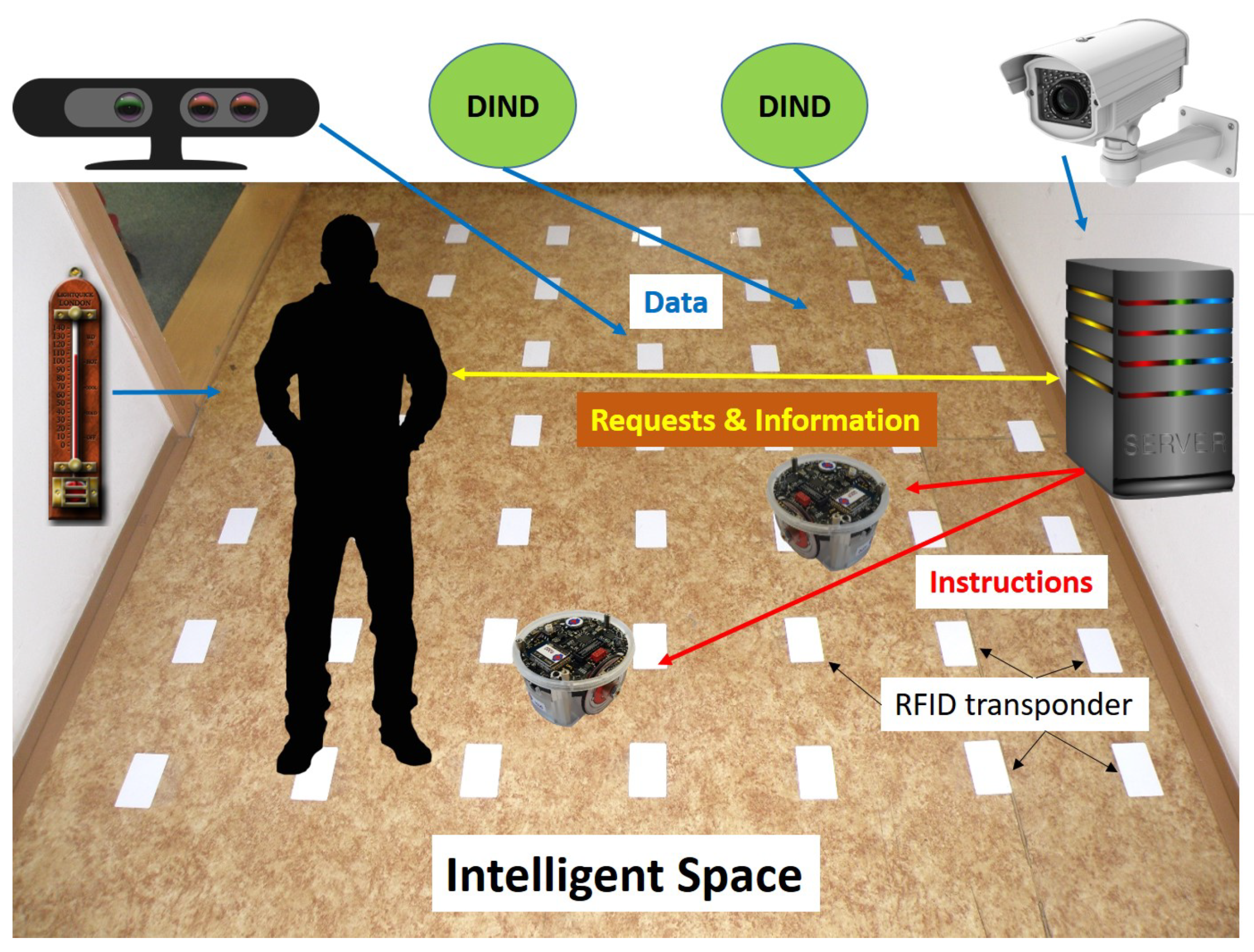
From the mentioned features of DLs, data processing needs a certain structuralization, and a part of calculations needs more powerful computational capacities, which may not be available onboard. Therefore, DLs need to use the advantages of both concepts, IS and IoT. Similarly, as things represent a basic IoT element, the so-called Distributed Intelligent Networked Device (DIND) plays the same role in IS, see Figure 2. One of the differences between DIND and thing is the distribution of computational power. While typical things such as thermometers, PIR sensors, or light detectors are also used in IS, there are even more complex devices like intelligent cameras, depth scanners (e.g., Kinect or Asus), or data and computational servers. Compared to IoT, a human often plays an active role in IS and is not only a recipient of services. Another difference between conventional IoT and IS is that IS is usually a relatively closed system, determined mainly for indoor applications. Compared to IS, the distribution of elements is much more extensive, the scalability is higher, and the number of elements is greater for IoT. The demands regarding the simple scalability of an IoT solution are stricter than in the case of IS. Finally, all these aspects lead to structural differences between IoT and IS, that is, the IS network is at least partially structured and centralized with a clear hierarchy of individual clusters of DINDs. Therefore, sensed data are in a more compact form. This fact is an advantage in data processing as very complex and sophisticated calculations are needed for robotic applications compared to IoT, although some exceptions exist. The complex nature and interconnections among elements of IS are also underlined by the existence of the so-called response loop, where a closed chain between sensors, data processing, decision-making, actuators, and again sensors can be observed [56]. In general, IS can be used for most robotic problems like navigation, human-robot interaction (e.g., guiding visitors), monitoring (e.g., hospitals and security), and smart environments like smart homes and smart factories.

UR, often named also as Ubibot, consists basically of three parts—virtual robot, real robot and sensory system, also known as Sobot (software robot), Mobot (mobile robot) and Embot (embedded system), respectively. Just the last mentioned part, Embot, represents the modified IoT environment in the form of IS [12].

When UR knows the complete state in IS, the situation offers further possibilities regarding predictions, decision-making, and modelling and better manages such a robot, that is, Mobot. Sobot represents extracted properties of Mobot and IS as well. It is practically their digital twin, and therefore, it should be able to do not only the same operations on the simulation level as Mobot in the real environment but also to provide a possibility of changing various parameters of Mobot and IS regarding space, construction or time to examine alternate solutions. It should contain methods solving topics such as self-learning and decision-making, which are based on artificial intelligence to offer at least the decision-making support for Mobot if not even direct control instructions.

Embot is IS modified for robotic applications, where the data are not only sensed but also processed and sent to Sobot and Mobot. Usually, Embot performs tasks such as localization of objects, evaluating the current situation, and delivering some instructions for Mobot. It represents a communication framework for the whole UR. Summarizing, the most typical relationship between these three basic parts of UR is to receive data from Embot and instructions from Sobot for needs of Mobot.

3.2. Distributed Localization

Although robots use their cameras as typical means for their localization, there are many situations when they cannot be used or their use is insufficient. This may include situations where the visual conditions do not allow their use, or the application also needs to know the situation outside their range, that is, to see behind the corner. Besides, some other reasons as security, computational complexity with relation to image processing and scene recognition can hinder their use. However, IoT offers other possibilities, even using sensors, which are primarily used for other purposes. Here, we will deal with radio and sound transmission devices, that is, Radio-Frequency Identification (RFID), radio beacons, and sonar.

RFID is composed of two basic elements, a reader (interrogator) and usually a set of tags as transponders. There are two basic types of transponders—passive and active. A passive transponder receives by its antenna the energy of radio waves emitted from a nearby reader (see Figure 3), which is again transmitted together with its unique Electronic Production Code (EPC). If the reader is in the vicinity of such a transponder, then it will get back its signal and EPC. Thus the reader plays a role of a transceiver. An active transponder has a battery, which is utilized to transmit EPC on a larger distance. For localization, mainly passive transponders are used as their range is usually only in centimeters, and so a relatively accurate position is determined. In [15] a network of RFID transponders deployed on a floor was proposed. Each position of a transponder with its unique EPC is recorded, so a map consisting of nodes representing individual transponders can be created. If a robot or vehicle with a mounted reader comes close to a transponder, then it marks its EPC. With the help of the aforementioned map, its position can be determined. The range of transponders gives the maximum accuracy of such a network because their signals must not overlap. Mostly, to secure a full but disjunctive cover of RFID signals, it is necessary to deploy about 20 transponders per 1 m${}^2$. If the network is too sparse, then the reader does not receive signals of transponders at every time step and, therefore, some approximate estimation will be needed. Either the next step is predicted based on the previous movement, or odometers deployed onboard are used. These are again burdened with an accumulative error, and so their probabilistic model will be required to correct it [19].

Another way to use RFID technology is to apply active transponders, whose range is from ten up to hundreds of meters, so they can also be used outdoors in some special cases. Active transponders are deployed only in important places like corners, obstacles, or other significant objects, which are visible enough, and their signal can spread with minimal interference. In this case, the so-called Radio Signal Strength Indication (RSSI) approach is used [57], where the strength of the transmitted signal is measured and compared to its original power. The farther the signal from its source is, the weaker its strength is. Knowing distances from several signal sources of transponders and using trilateration, we can calculate such a reader’s position. However, the quality of an RFID signal is quite low because of its instability. To minimize this drawback, radio beacons, especially products based on the protocol iBeacon utilizing BLE technology, which steadily transmits EPCs with better signal stability, are used. However, radio beacons are also affected by various interferences and deformations caused by a given environment. Laborious calibration of all beacons is also needed as shown in [16].

Therefore, to obviate calibration, an idea to combine these devices (RFID as well as beacons) with other types of devices based on different physical principles comes into account. Mainly odometers and sonar devices could be suitable candidates because of their complementary properties with radio-based devices. Further, we will focus on the combination of the radio (RFID and beacon) and sonar technology and comparison based on the propagation of their waves. Radio waves extend radially in all dimensions and more or less penetrate the area, including potential obstacles. Although high-frequency signals penetrated through obstacles show high energy, damping an unambiguous detection of objects (e.g., obstacles) is problematic. On the contrary, sonar waves extend conically and are reflected from any objects. To summarize, radio waves are blind regarding obstacles, and sonar waves are blind outside the signal cone. Thus radio devices can be used for direct localization of a mobile robot if passing individual transponders, and a sonar performs object detection to prevent a collision with an obstacle, see Figure 4.

As the modelling of radio waves propagation and related RSSI approaches is quite complicated, we will deal only with using a sparse network of passive RFID transponders. If a mobile robot loses a signal from all transponders, then the position change of objects sensed by the sonar can be recalculated to a new position of the robot. Thanks to the small dimensions of RFID transponders and their low prices, it is pretty straightforward to deploy them in high numbers to cover larger spaces.

For successful navigation, we generally need to know three kinds of information: robot position, at least the positions of immediate obstacles, and the position of a goal. The task is to find a path between the robot and the goal, which will avoid all obstacles. The path can be constructed at once if knowing the whole situation or incrementally. Usually, reactive navigation creates its path incrementally, and so it minimizes computational complexity. As reactive navigation can be easily described in rules expressing relations between the mentioned three kinds of information and this information are affected by errors, in reality, it seems to be advantageous to use fuzzy logic [58]. In the next section, we will show the use of FCMs for this type of problem.

4. Fuzzy Cognitive Maps and Their Adaptation

Although FCMs were originally proposed for modelling social and biological processes [59], thanks to their user-friendliness, they have also spread to technical applications during the last decade. Two main reasons exist. Firstly, FCMs offer a very transparent representation of relations among objects. As they can be regarded as an extension of fuzzy production rules, their advantages will be emphasized if variables cannot be exclusively divided into either input or output ones. In such a case, the use of rules loses its representativeness and comprehensiveness. Therefore, FCMs are especially suitable for the description of relations typical by chained rules and closed loops. Secondly, properties of FCMs like stability and convergence, which are very important for technical areas, can be relatively easily analyzed.

FCMs are oriented graphs, where the set of nodes C represents notions in a symbolic form and causal relations are in the form of weighted connections. Mostly, notions are objects described by states or conditions, and connections are actions or transfer functions, which transform a state in a node to another one in another node. As FCM can be regarded as a set of rules so input nodes represent parts of a rule the premise, which is interconnected with the output node, whose value corresponds to the rule consequent as we can see it in Figure 5.

The connection between an input node $c_i$ and an output node $c_j$ can be weighted by a value $e_{ij}$ from the interval $[-1;1]$ (−1—because of negative connections) and so we can implement grades of membership into the inference process in the form of weights. If we define initial numerical state values $a_i$ in nodes $c_i$ from the interval $[0;1]$ then using (1) we can calculate new state values for next time step $t+1$:

$$A(t+1)=L\left(A\left(t\right)+A\left(t\right).E\right)=\left\{L\left(a_i\left(t\right)\sum _{j=1}^n{e}_{ij}\times a_j\left(t\right)\right);i=1,\dots ,n\right\},$$

(1)

where A is the state vector of individual nodes $c_i$ with their state values $a_i$. E is the connection or adjacency matrix of weighted connections $e_{ij}$. L is the limitation function to keep the values $a_i$ in [0;1]. Thus we can simulate behaviour of an investigated system and then we can analyse its properties. Therefore, FCMs can be very useful especially for prediction purposes [59].

However, such an FCM is a closed system as there are no input nodes for external values, that is, any outer influence is excluded. This is a very strong limitation for technical systems, and therefore, a modification of FCMs is needed, which consists in implementation of input nodes for external values, where input values $i{n}_i$ are evaluated by membership functions being defined in these nodes and their activation values are in the form of grades of membership. They are analogous to the compatibility calculation in conventional fuzzy controllers. Thus the inference process defined in (1) is modified to the following form for calculating the elements $a_i\in A$:

$$a_i(t+1)=\left\{\begin{array}{cc}{\mu }_{A_i}\left(i{n}_i\left(t\right)\right),\hfill & \mathrm{if}i{n}_i\mathrm{exists}\hfill \\ L\left(a_i\left(t\right)+{\displaystyle \sum _{j=1}^n}{e}_{ij}·a_j\left(t\right)\right),\hfill & \mathrm{if}i{n}_i\mathrm{does}\mathrm{not}\mathrm{exist}\hfill \end{array}\right..$$

(2)

As already mentioned, the design of an FCM, that is, the definition of nodes and connection weights, is not trivial and still requires to manually propose the set of nodes and at least the basic topology of FCM. All known adaptation methods of machine learning focus exclusively on the design of the connection matrix. The problems connected with the use of most known adaptation methods like genetic algorithms and methods typical for neural networks are described in [60]. The methods are not as successful when utilized for FCM, as in the case of neural networks, and there is a reason to search for more convenient methods. Recently, two approaches from the group of evolutionary algorithms, namely migration optimization and particle swarm optimization have gained broad interest and use in various application areas. In contrast to genetic algorithms, no new population will be generated, and during the whole optimization process, the same individuals will remain. Thus, all collected knowledge will be preserved. We can observe certain direct learning during optimization, unlike indirect learning in genetic algorithms—selecting the best individuals and subsequent transfer of their genes to future generations. This paper aims to focus on using these two approaches for FCM adaptation and considering their potential in this area.

4.1. Migration Optimization in Adaptation of FCM

Migration optimization is motivated by some animals living in groups like wolves in packs, where wolves search for prey collectively. The pack has a leader who is the most successful individual. Here, we will deal with the so-called Self-Organizing Migration Algorithm (SOMA) [61] as a special representative of this approach.

SOMA is based on cooperative searching (migrating) the area of all possible solutions. Individuals are mutually influenced during the search process. This fact leads to forming and dissolving groups of individuals, which organize the movement of individuals and so the search area can be reduced quicker than in the case of genetic algorithms. Another advantage of this approach lies in the ability to process various data types of parameters like integers, real or discrete values, and also mutually mixed ones. To generate an initial population the so-called specimen S is defined at first, which is a set of allowed values for D variables to be optimized:

$$S=\left(s_1^{Type}(s_1^{LL},s_1^{UL}),\dots ,s_D^{Type}(s_D^{LL},s_D^{UL})\right),$$

(3)

where $Type$ represents the data type of a variable, $LL$ and $UL$ are its low and upper values, respectively.

The principle of SOMA is based on following a leader of such a group (pack), who has the best fitness value, by other members (individuals) of the group. A member and the leader are interconnected by a movement vector $\overrightarrow{m}$ constructed over the fitness function (see Figure 6) and at given points $I_k$ of this vector defined by the parameter $Step$ the fitness is calculated and saved in the memory. $Step$ represents a particular length of $\overrightarrow{m}$, where $k=0,\dots ,n$ and $\parallel \overrightarrow{m}\parallel =n·Step$. To better cover the search space, the given individual should precede the leader’s position in a forward direction and stop searching at the final point $Mass·\overrightarrow{m}$. The parameter $Mass$ is a dilatation coefficient of $\overrightarrow{m}$ between the initial position of the individual $I_0$ and its final position $I_f$ ($f=Mass·n$) in the frame of one migration cycle.

Similarly as in genetic algorithms, also SOMA has analogous operators, namely perturbation $PRT$ and migration. The perturbation corresponds to the mutation but the result is not a change of a given individual. However, only its $I_f$ is modified, that is, the individual will not directly follow its leader but a certain deviation from $\overrightarrow{m}$ will occur, see Figure 6. As $\overrightarrow{m}$ is calculated as a difference of vectors ${\overrightarrow{r}}_L$ and ${\overrightarrow{r}}_0$, that is, vectors of the leader L and starting point $I_0$ of the given individual, respectively then the real position of $I_f$ will be modified (perturbed) as follows:

$$\overrightarrow{r}={\overrightarrow{r}}_0+p.\widehat{m}\ast {\overrightarrow{v}}_{PRT},$$

(4)

where $\widehat{m}$ is the unit vector of $\overrightarrow{m}$ and the vector length p relates to the order of steps k on a path of the given individual I from the starting point $I_0$ (${\overrightarrow{r}}_0$) to the final one $I_f$ ($\overrightarrow{r}$), that is, $p=k.Step$, $k=0,1,\dots ,Mass·n$. The elements of the perturbation vector ${\overrightarrow{v}}_{PRT}$ are created in each migration cycle by a condition: $\mathrm{if}{\mathrm{rnd}}_j<PRT\mathrm{then}{\overrightarrow{v}}_{PRT,j}=1,\mathrm{else}{\overrightarrow{v}}_{PRT,j}=0$, where ${\mathrm{rnd}}_j$ is a randomly generated number and j is the index for a given property ($j=1,\dots ,D$). The vector ${\overrightarrow{v}}_{PRT}$ (${\overrightarrow{v}}_{PRT}=({\overrightarrow{v}}_{PRT,1},\cdots ,{\overrightarrow{v}}_{PRT,D})$) is in reality a mask and the operation * performs pairwise products among individual elements of $\widehat{m}$ and ${\overrightarrow{v}}_{PRT}$. If $PRT$ has a small value then ${\overrightarrow{v}}_{PRT}$ will have mostly zeros and the perturbation will affect direct movement of a given individual to the leader, that is the movement vector $\overrightarrow{m}$ will be modified. Only the dimensions, where values of ${\overrightarrow{v}}_{PRT,j}$ are adjusted to 1 will not be perturbed and the movement will be similar to the original form of $\overrightarrow{m}$, see Figure 6.

Similarly, migration is analogous to crossover in genetic algorithms. During one migration cycle, (4) is evaluated in k points, where their fitness is investigated and saved in the memory. Although no new population is created, this representation is equivalent to a sequence of descendants depicted in Figure 6 as bullets (one step—one descendant). After the migration cycle, all individuals will come back to their best-found positions. Eventually, the leader will be replaced by the individual with the best fitness, and a new migration cycle will start. This mechanism corresponds closely to the selection in genetic algorithms. Generating new populations is substituted by migrating individuals during migration cycles in the state space.

In the case of FCM adaptation, one way is to define individuals as a connection matrices E and to let them compete mutually. The question is how to generate candidate connection matrices in the initial step. Maybe, the simplest possibility is to set-up all elements for one individual in E to 1 then E of another individual for example, to 0.9, and so forth, to cover the whole range of weights in $[-1;1]$. During the optimization process, due to permutations, the values of weights in E will reach ample variability and will converge to an acceptable quality of FCM performance for a given application. If we know what connections will not exist at all then E can be reduced to a simple list of connections with non-zero weights. Thus, the computational complexity of the optimization process will be significantly reduced.

4.2. Particle Swarm Optimization in Adaptation of FCM

PSO approach can be principally also affiliated to the part of MAs because, analogously to SOMA, no new generations are created, but all acquired knowledge is collected in the memory of an individual. In this case, PSO was motivated by swarms of birds, and its model is suited for modelling swarms. Individuals are in the form of particles, which are searching for better results. PSO utilizes the so-called social dynamics as well as emergent behaviours being arising from colonies organized on social laws. No DNA-inspired operations are used on the population. PSO behaviour is analogous to SOMA in many aspects because it considers the best results of individuals and the best result of the swarm as a whole. A leading member also exists in a swarm [62]. Each particle moves in the search space and tries to find the best solution adjusting its trajectory according to its memory (where the solutions are stored) as well as the memories (solutions) of other particles. In comparison to SOMA, the knowledge sharing among particles is more intense. The particles move with adjustable velocity and remember the best personal position achieved, that is, where the best solution was found. Depending on a given type of PSO, the best position found by all individuals, hence by the entire swarm, can be shared by all particles.

Supposing a D-dimensional search space, then the position of a particle $X_i$ can be determined by a D-dimensional vector, $X_i=\left(x_{i1},x_{i2},\cdots ,x_{iD}\right)$. Analogously, its velocity is defined as $V_i=\left(v_{i1},v_{i2},\cdots ,v_{iD}\right)$. Further, we expect that each particle has the information about its best individual result (position) $P_i$ obtained during its whole history and also about the best global result of the swarm $g_i$. The velocities and positions of particles are modified as follows [62]:

$$X_i(t+1)=X_i\left(t\right)+V_i(t+1),$$

(5)

$$V_i(t+1)=\chi \times \left[V_i\left(t\right)+C_1\times R_1\times (P_i\left(t\right)-X_i\left(t\right))+C_2\times R_2\times (P_{g_i}\left(t\right)-X_i\left(t\right))\right],$$

(6)

where the parameters $\chi ,C_1$ and $C_2$ are constants named as constriction factor, social and cognitive parameter, respectively. Vectors $R_1$ and $R_2$ are random, whose parameters are analogous to mutations and are from the interval $[0;1]$. In general, the initialization of the swarm is very important to maximize the quality of the optimization process, especially its convergence speed and quality of final results. Now we need to modify the described general PSO approach for the needs of FCMs. In [63] such a modification based on a certain similarity with the learning of neural networks was proposed. The goal is to design a FCM with such a connection matrix E, which brings the FCM to a stabilized position, hence after a certain time its nodes will keep their activation values$a_i$ in prescribed limits $a_i\in [a_i^{min};a_i^{max}]$. The search space dimension D is given by the size, that is, the cardinality of E, but it can be decreased by the number of zero elements in E if we know this kind of information in advance. The coordinates $i=1,\dots ,D$ of such a space are assigned to individual weight elements of E. Therefore, the input argument for the fitness function $F\left(E\right)$ will be E and $F\left(E\right)$ is defined as follows [63]:

$$F\left(E\right)=\sum _{i=1}^{m}H(A_i^{min}-A_i)\times \mid A_i^{min}-A_i\mid +\sum _{i=1}^{m}H(A_i-A_i^{max})\times \mid A_i^{max}-A_i\mid ,$$

(7)

where H is the Heaviside function ($H\left(t\right)=0$ if $t<0$ else $H\left(t\right)=1$). The goal is to minimize $F\left(E\right)$ and subsequently to determine the conjoint E.

However, the mentioned PSO modification does not solve the problem of proper swarm initialization. Suitable distribution of particles over the search space is the first condition to achieve a good initialization. A suitable geometrical object with its vertices could help obtain the required distribution of particles. There are methods using, for example, hypercubes [64,65], but they cause generating a very high number of vertices, that is, particles, because they grow exponentially ($2^D$). Therefore, we have proposed to rather use a D-dimensional simplex, which generates only $D+1$ vertices, that is, the growth of their number is linear. Moreover, the convergence of PSO process can be accelerated twice if we use two symmetrical simplices producing vertices in parallel.

5. Route Tracking System for UR—Description and FCM Design

This section will show the presented methods of FCM adaptation on an example of reactive navigation for needs of route tracking, which was already partially solved in [65], but without means of IoT. As the proposed environment and the way of data processing correspond more to IS’s idea (see Section 3.1), we use the concept of UR for solving this problem.

Let us suppose a route in the form as depicted in Figure 7, where we can see a movement of a robot or vehicle, in general. The task is to keep the robot within the borders for the whole route. If a robot exceeds these borders, then a collision occurs, but it can still come back to the route as it is also this case. The worst situation will happen if the robot totally leaves the route, that is, it diverges from the solution.

The task and main criterion are to eliminate or at least minimize such situations of collisions or even divergent behaviour. Besides, other criteria can be considered, which relate to the movement trajectory’s quality or energy consumption. To solve this task, we need some kinds of data, which result from the analysis of a route as seen in Figure 8. In order to keep a robot in route borders effectively, a centerline (dash-dotted line) is defined, and we try to minimize deviations of robot positions from this centerline. In other words, we try to track the robot along this centerline. For this reason, the route is divided into smaller parts corresponding to control sampling, so we get a set of reference points $rp$ deployed on the centerline and depicted as yellow bullets. There are at least two variables, which are necessary for route tracking. Firstly, it is the distance of the robot $x_1$ from the reference point $rp\left(t\right)$ in time t. Secondly, it is the centerline’s angular deviation—the angle $x_2$ between the robot orientation, that is, movement axis, and the next reference point $rp(t+1)$. For a more realistic control, other variables are also suitable, especially variables for a description of the route’s physical properties to prevent, for example, slips.

As seen, measuring $x_1$ and $x_2$ with the use of exclusively onboard sensors is not trivial. The simplest measurement relates to the angle $x_2$. If the centerline and its reference points are marked on the road surface, it will only be necessary to focus a rotational detection device (such as a camera) on $rp(t+1)$. The turning of the camera from the movement axis of the robot will be just $x_2$. Measurement of $x_1$ is more complicated because it requires measuring the distance between the position of the robot in time t and $rp(t+1)$ as well as the azimuth of the movement axis to $rp\left(t\right)$. Let us suppose we know the positions of individual reference points and their mutual distances. In that case, we can calculate the angle between $rp\left(t\right)$ and $rp(t+1)$ related to the vertical coordinate of $rp\left(t\right)$ using the minimal horizontal distance $md$ between these two points. Finally, we will calculate the remaining angle in the triangle between such a robot’s actual position and both neighboring reference points, so we will get $x_1$ using the cosine formula. Such a calculation is not only complicated but, after so many calculation steps, also affected by a considerable error. Furthermore, to measure distances and azimuth, we need a rangefinder and still another detection device for $rp\left(t\right)$. Both devices are relatively expensive. There is also a question, how to implement markings for reference points, or to be more precise, how they will be detected.

Therefore, it is more advantageous and simpler to distribute detection devices along the route than in the previous onboard solution. There are principally two possible approaches. The more precise way is to construct gates consisting of passive RFID transponders; see green bullets in Figure 8. The only onboard device is the RFID reader. Another solution is to distribute beacons at least along one side of the route. In this case, the onboard device is a BLE reader with the RSSI functionality. For a more accurate calculation, the beacons should be distributed on both roadsides, and so they will create virtual gates. These readers’ task is to detect the intersection of the movement axis and the gate, where distance $x_1$ can be directly measured. To calculate the angle $x_2$, we need to know the movement axis, which can be constructed using intersections at gates $t-1$ and t. Then we will construct two right triangles. One of them is constructed between intersections with the movement axis at gates t and $t+1$ using $md$ and another one between the intersection at the gate t, $rp(t+1)$ and again using $md$. The angle $x_2$ is divided between these two triangles. As the side lengths of these two triangles can be calculated from the mentioned intersections, we can calculate the angles $x_2^{\prime }$ and $x_2^{″}$ using basic trigonometric functions and the final angle is their sum, that is, $x_2=x_2^{\prime }+x_2^{″}$. The approach utilizing RFID transponders can achieve the accuracy of several centimeters, and the approach with beacon technology can achieve the accuracy of several tens of centimeters. Another advantage in the case of outboard devices is a much simpler calculation with more precise measurements. The measurements of angles are especially affected by serious errors, but in the IoT version, they are not measured at all.

In navigation, input variables usually express the position of a robot and its change related to other objects (mainly obstacles) as well as to the goal. In this case, they are position deviation, that is, the distance to the reference point at a given time step ($x_1$), which should be zero in the ideal case, and angular deviation, that is, the angle between the movement axis and the next reference point ($x_2$). Regarding the control quantities, they depend on various properties of a given vehicle or robot, that is, if they are wheeled or stepping, but generally, they depend intrinsically on turning and speed of the movement [66]. For simplicity, let us suppose navigation of a wheeled robot, but this approach can be used for any kind of robotic movement. Therefore, the outputs will be both the change of speed—acceleration or deceleration and the turning of such a robot—its angle of turn. 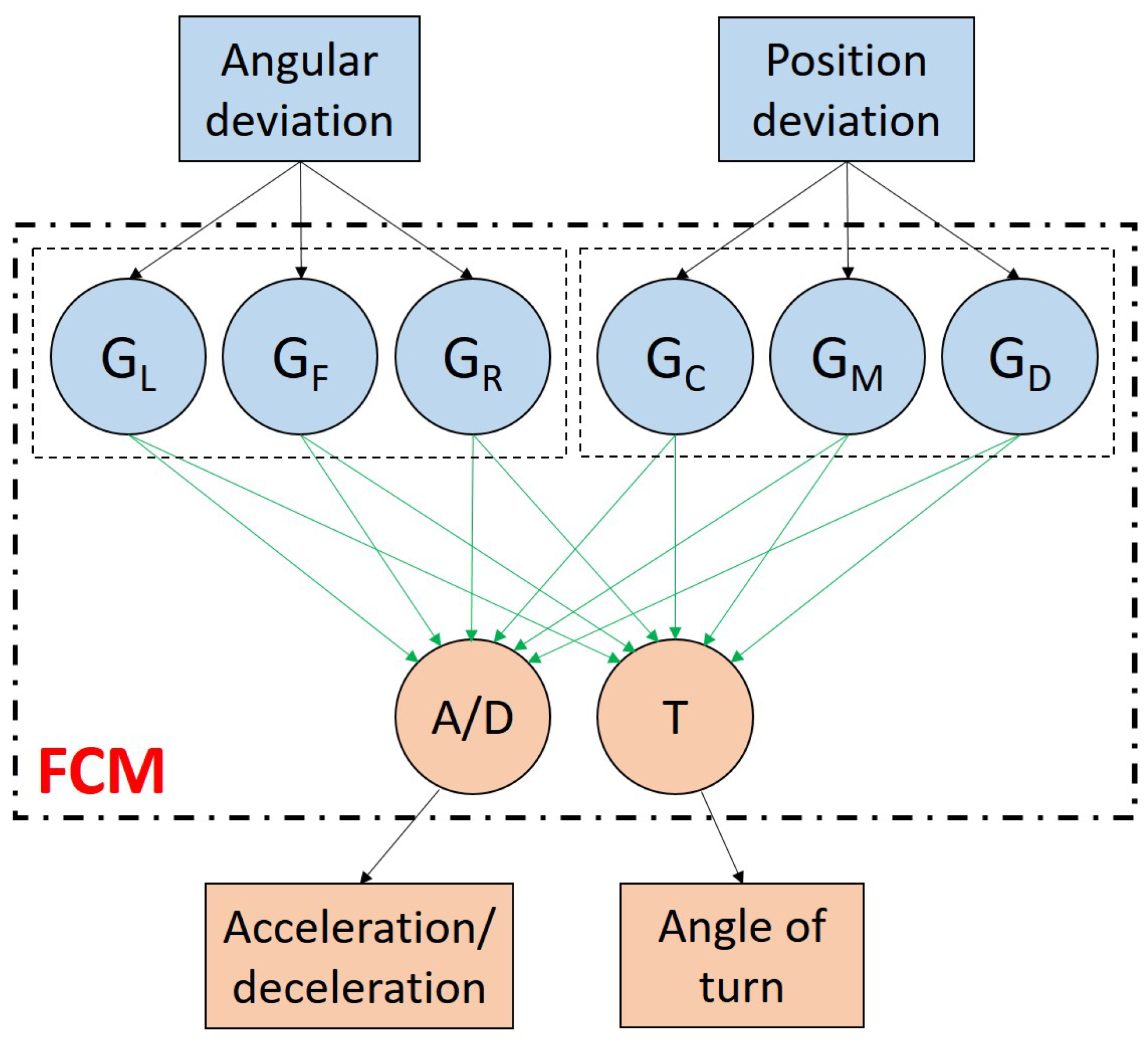Such a frame of questions will then issue to the architecture design of a navigation system, in our case in the form of FCM, which is depicted in Figure 9.

It is evident that outputs will depend mainly on the robot’s position against the position of a goal. In this case, the proposed FCM will function in a loop when individual goals are identical to reference points, which follow one after another in each time step. Therefore, individual symbols stand for the following: D—distant, M—medium, C—close, R—right, F—forward and L—left. These nodes express the angular position ($G_L$, $G_F$, $G_R$) and the distance ($G_C$, $G_M$, $G_D$) of a robot against a preliminary goal, respectively. Their activation values are calculated in the form of grades of membership, which are based on manual definitions of membership functions placed directly in the nodes, see Figure 10.

Although the FCM topology and membership functions of input nodes for external values must be defined manually, there is still the possibility to automatically set-up weights of connections—the connection matrix E. As there are 8 nodes in total, then E will have the dimension $8\times 8$, but we will need to adjust only 12 connections (see green arrows in Figure 9).

6. Experiments and Their Evaluation

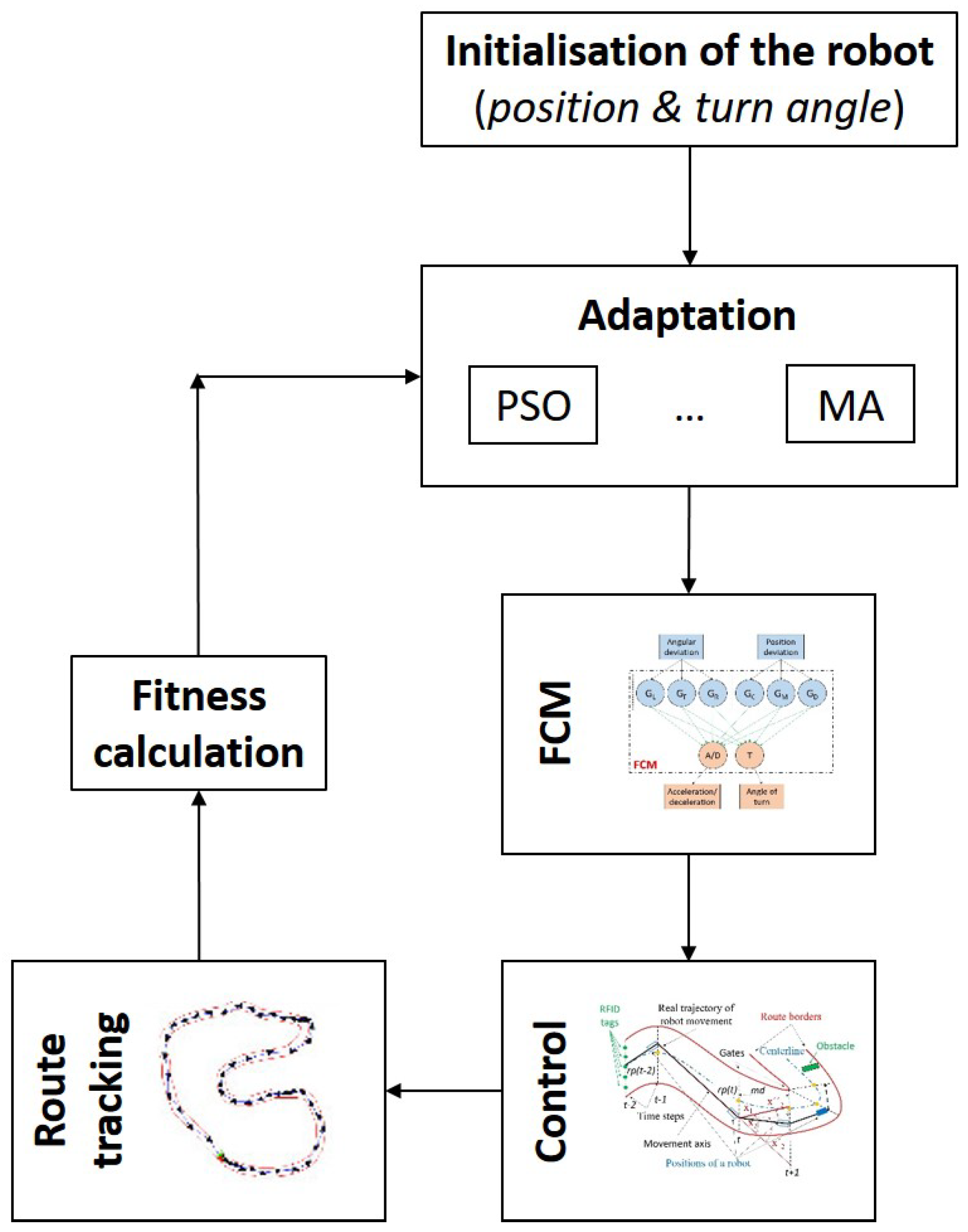
To verify our idea to use FCMs for route tracking in the environment of IS and to use the concept of UR we did a series of simulation experiments, where two basic FCM adaptation approaches, that is, SOMA and PSO, were applied for adjusting the connection matrix E. Their results were compared together with a manually designed FCM with the help of calculated fitness values for each FCM design. The chosen research and experimental methodology are depicted in Figure 11.

After the initialization, if the robot is deployed at a certain position in the route and under a given direction (angle) against the closest reference point (see Figure 8), a loop of calculations will be started. It consists of generating E using one of the offered algorithms by the adaptation block (PSO, SOMA, or something else). Then the adjusted navigation FCM will control the robot movement based on the means of IoT described in Section 5. It generates two control values—acceleration and angle of turn. After applying the control values by the actuators of the robot (wheels or joints), the robot will move to a new position until it achieves the final reference point. In our experiments, we used closed routes, that is, the starting point is also the final one, but it is not necessary. After the route tracking is finished, the fitness value $F\left(E\right)$ will be calculated using (8). This loop will be repeated as many times as there are individuals in a given population. In such a way, the calculation of candidate solutions will be completed for one generation. If the best solution fulfills the required conditions, then the adaptation process will be finished; otherwise, a new generation will start. This calculation will be repeated until the required conditions are satisfied, or the maximum number of generations is achieved. Another stopping criterion is the minimal change of $F\left(E\right)$ during the adaptation process, too.

As both approaches belong to the evolutionary computation before we start with the optimization, it is necessary to define the fitness function, which takes into account the following criteria [65]:

• mean angle of turn,
• mean acceleration,
• trajectory length,
• mean speed,
• passing time,
• number of collisions with route borders,
• passing the route (yes/no or 1/0).

In this case, the fitness value $F\left(E\right)$ expressing the quality of a proposed connection matrix is defined as follows:

$$F\left(E\right)=1/(p_{at}\times at+p_a\times a+p_{tl}\times tl+p_s\times s+p_{pt}\times pt),$$

(8)

where $p_{at}$, $p_a$, $p_{tl}$, $p_s$ and $p_{pt}$ are parameters for mean angle of turn $at$, mean acceleration a, trajectory length $tl$, mean speed s and passing time $pt$, respectively. Their values depend on user’s preferences. The mean values (angle of turn, acceleration, and speed) are considered as absolute values.

The greater the value of $F\left(E\right)$, the better quality of E will be achieved. In other words, we are searching for the maximum value. The reason for such a definition of $F\left(E\right)$ is, if the robot diverges from the route, then it will be lost, and $F\left(E\right)$ will be set-up to 0 (at all the worst fitness value). Principally, we have two possibilities how to handle such a particle in PSO or an individual in SOMA. Either the particle/individual will come back to its previous best position, or it will be removed and replaced by a new one at another position. In our experiments, we choose the second alternative to improve adaptation methods’ exploration ability, in general. Finally, if the route’s borders are exceeded, then $F\left(E\right)$ will be divided by 2 as many times as the borders are exceeded.

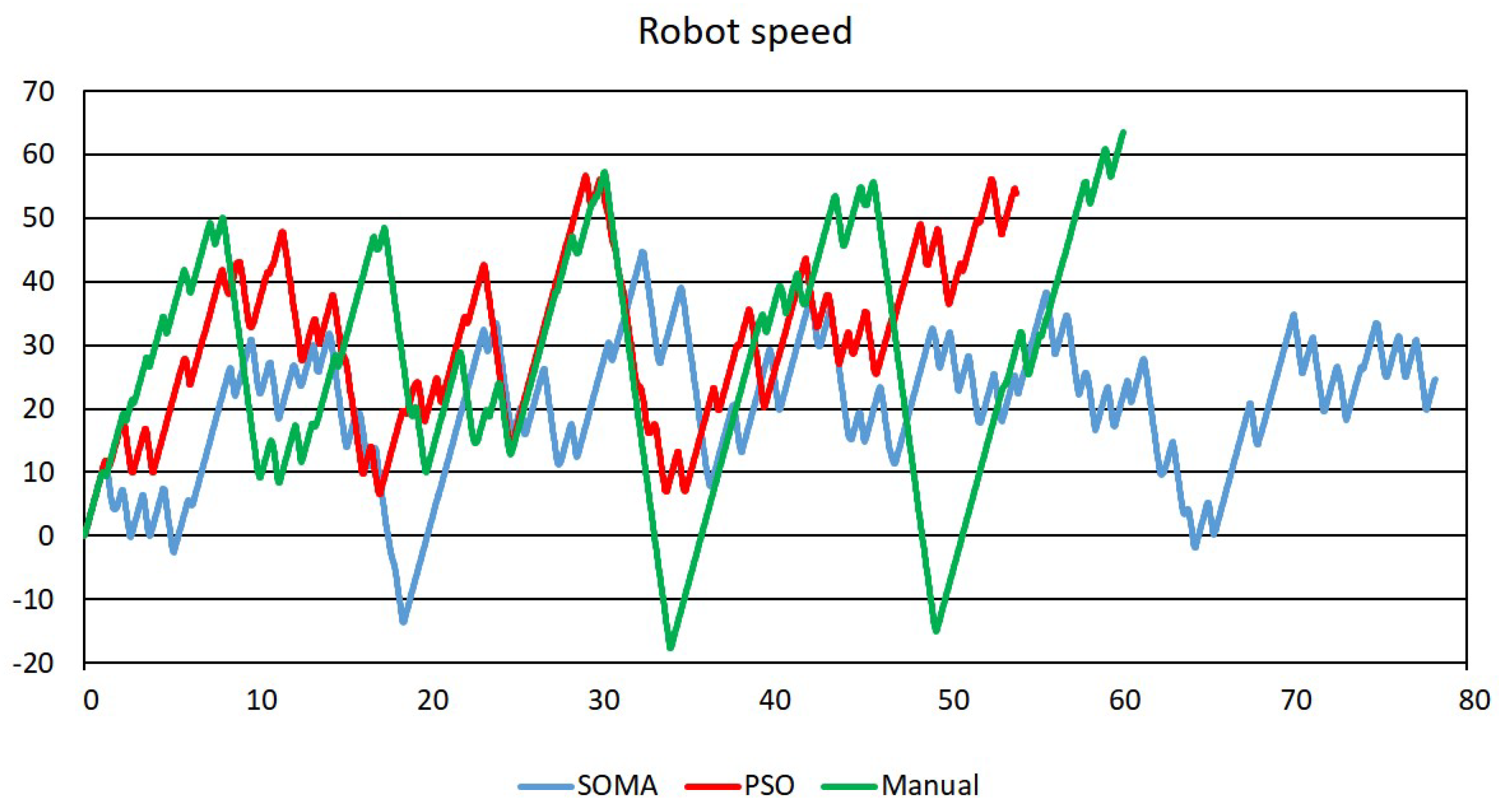
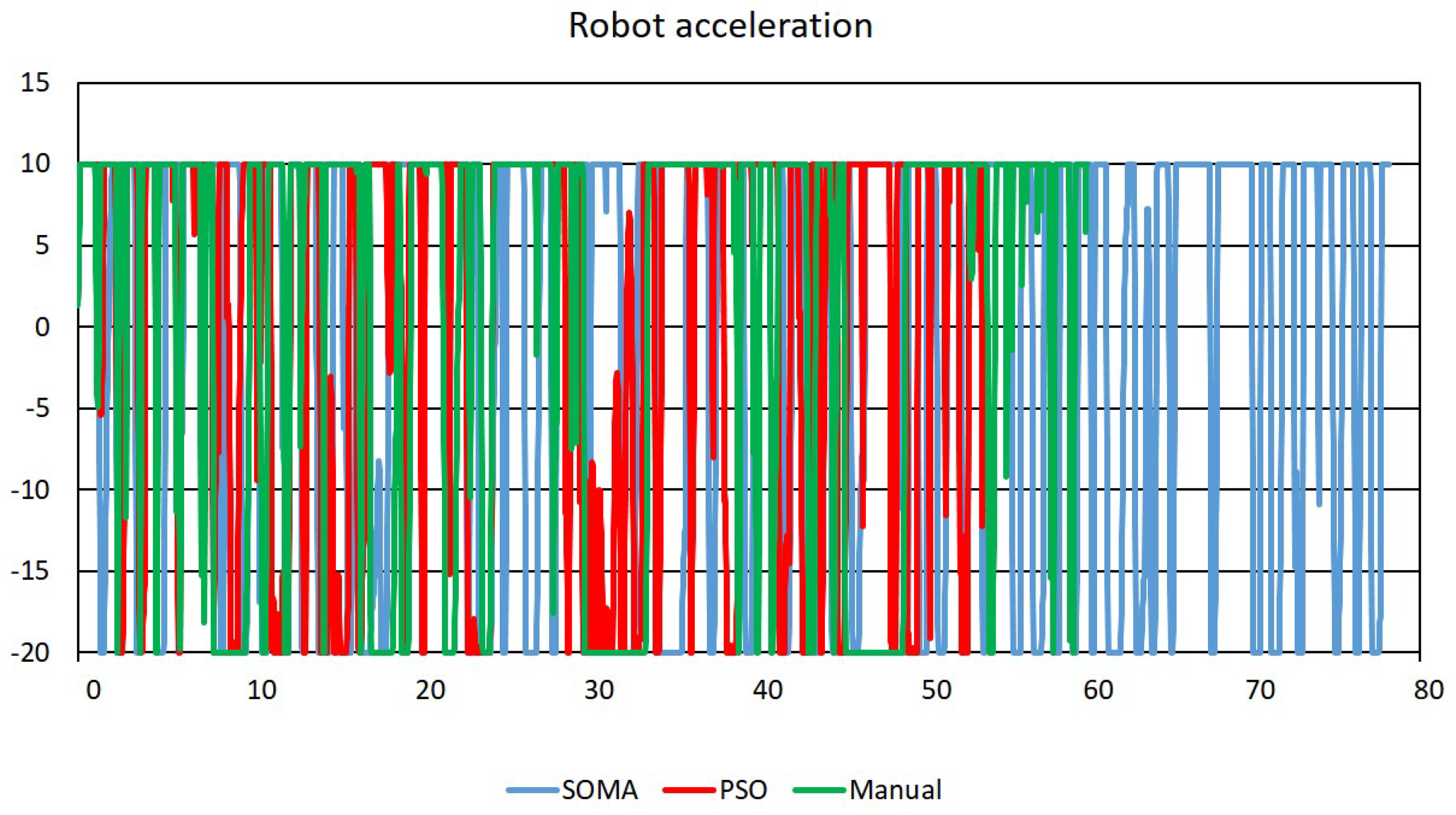
Figure 12, Figure 13, Figure 14 and Figure 15 depict behaviour of first five variables mentioned in the list of criteria for the calculation of $F\left(E\right)$, namely: trajectory length (cm), robot speed (cm/s), robot acceleration (cm/s${}^2$), angle of turn (${}^{\circ }$), and passing time (s), which represents their horizontal coordinates.

The comparison of these variables points to the quite different behaviour of FCMs designed by PSO and SOMA even though there is only a slight difference between their fitness values, see

Table 1. Quality comparison of selected FCM adaptation methods.

Quality Criterion	FCM Adaptation Method
	Manual	SOMA	PSO
Relative optimization process length	-	1	5.72
Number of generations	-	20	186
Number of individuals	-	41	26
Relative fitness	1	1.45	1.52

. The FCM controller designed by SOMA causes a slower but a little more stable movement (see Figure 12), whereas the PSO design also utilizes extreme control values resulting in higher speeds (see Figure 13). If we compare differences of fitness values among individuals in SOMA, they are smaller than in PSO, that is, the SOMA optimization process produces more stable results compared to PSO. On the contrary, it has a more significant disposition to stack in a local extreme because SOMA exploration is more systematic and spreading individuals less stochastic than in PSO. This fact could explain the obtained results when the SOMA design produces a stable behaviour with minimal extremes. In other words, PSO, thanks to its stochasticity, shows better exploration than SOMA.

Figure 14 and Figure 15 highlight that FCM is indeed able to control the robot inside a route, but extreme changes of the acceleration and turn angle are needed. However, thanks to the ability to back the robot, it is able to move along complicated routes, as shown in Figure 7. Therefore, future research will deal with this disadvantage and will aim to mitigate the need for extreme actuating.

The methods of automatic adaptation of FCMs in comparison to the manual design clearly show their superiority. It is visible mainly in Figure 13, where manual design uses the most extreme speeds for controlling the robot. Their strong changes are visible also in Figure 14 and Figure 15. In other words, FCMs designed with the help of PSO and SOMA are more favour to the controlled devices than the manual design, especially if we consider mechanical properties of such a robot or vehicle.

In the case of SOMA optimization, 41 individuals were created with values discriminated by 0.5 from the interval $[-1;1]$. As after 20 migration cycles, the difference in fitness values among individuals was not significant in most cases, we stopped the optimization process.

As already mentioned, the initialization is crucial in PSO and strongly influences the quality of the output, that is, E. Like SOMA, PSO has the same dimension of the search space, that is, D is equal to 12. We used a pair of symmetrical simplices, that is, the number of particles was 26 (2.(12 + 1)).

We repeated experiments with different forms of routes, but differences concerning the quality of used methods were not significant. Table 1 shows a comparison of averaged results acquired from a series of experiments, where the relative values of selected criteria describing properties of the optimization process were related to the smallest value.

The summary of the results shows that differences between SOMA and PSO approach are not significant. SOMA produced a slightly worse connection matrix than PSO, but the comparison of the computational complexity of the optimization is much more advantageous in the case of SOMA. Further, it is apparent that a small number of individuals requires a larger number of optimization cycles.

7. Conclusions

In this paper, we showed the possibility of interconnecting the concepts IoT and IS with the aim to construct UR. We showed how means of IoT could be used in navigation tasks as route tracking. Our approach tries to utilize a combination of IS and onboard robotic means to find a proper balance between these two groups of sensors.

Our approach represents an introductory study using quite new means in the area of navigation like IoT and FCMs. The pros and cons of our approach can be summarized as follows:

• Although the architecture of used FCM is quite simple, consisting of only 8 nodes, it was able to navigate a robot through a complicated route.
• The used adaptation methods proved their quality over a manual design.
• It seems, that PSO adaptation is suitable if we need an optimal or almost optimal solution and its stability does not play an important role. On the contrary, SOMA adaptation secures although a solution of mean quality, but it is stable and credible.
• The quality of tracking is considerably ’shaky’. The control changes the turn angle and speed too quickly and strongly. Such a navigation would have a negative influence on energy consumption and durability of such a device. The solution could be in extending the number of nodes, which enable to more accurately describe a given situation.
• The proposed navigation system can be implemented as a part of the simulation system for movement control in the frame of Sobot as well as a part of the control system in the frame of Mobot.

In the future, one of the most important criteria will also be the economic effectiveness of solutions. Our approach enables navigation also for simple devices not owning complex sensors. The strength of our proposal is also based on its scalability when an arbitrary number of robots will be able to use their common IS and mutually cooperate, including robots of different types, too. In this case, the emphasis will be on the functionality of Sobot because a massive amount of various simulations and alternatives will be necessary before real robots start their work.

The use of artificial intelligence techniques showed many advantages in robotic problems. For instance, fuzzy logic can describe uncertainties of localization means based on evaluating signal strength and designing decision-making systems using, for example, FCM. Neural networks can be used mainly to classify signals from several devices at once to prevent their interference. Finally, evolutionary approaches are very suitable optimization means as it was also shown in designing connection matrices for FCM.

In the future, other devices can be added to the proposed IS and we can properly combine onboard devices with outboard ones. Therefore, we will try to extend the UR concept in IS to collaborative robotics, where a number of robots cooperate on a given task.