Approximate Array Multipliers

Abstract

This article describes the design of approximate array multipliers by making vertical or horizontal cuts in an accurate array multiplier followed by different input and output assignments within the multiplier. We consider a digital image denoising application and show how different combinations of input and output assignments in an approximate array multiplier affect the quality of the denoised images. We consider the accurate array multiplier and several approximate array multipliers for synthesis. The multipliers were described in Verilog hardware description language and synthesized by Synopsys Design Compiler using a 32/28-nm complementary metal-oxide-semiconductor technology. The results show that compared to the accurate array multiplier, one of the proposed approximate array multipliers viz. PAAM01-V7 achieves a 28% reduction in critical path delay, 75.8% reduction in power, and 64.6% reduction in area while enabling the production of a denoised image that is comparable in quality to the image denoised using the accurate array multiplier. The standard design metrics such as critical path delay, total power dissipation, and area of the accurate and approximate multipliers are given, the error parameters of the approximate array multipliers are provided, and the original image, the noisy image, and the denoised images are also depicted for comparison.

1. Introduction

Approximate computing is considered to be a high speed, low power, and energy-efficient alternative to accurate computing [1]. Many applications of approximate computing have been discussed in the literature, which includes multimedia [2], hardware implementation of neural networks for artificial intelligence and machine learning [3], neuromorphic computing [4], big data and analytics [5], software engineering [6], memory systems for multi-core processors [7], graphics processing units [8], etc. Approximate computing includes approximate hardware, software, and memory storage. Approximate hardware covers approximate arithmetic circuits [9] and approximate logic circuits [10]. With respect to approximate arithmetic circuits, the designs of approximate adders and multipliers have been given much attention. This is understandable given that addition and multiplication are important arithmetic operations which are frequently performed in microprocessors, digital signal processors, and application-specific processors [11].

This paper deals with approximate multiplication. Many architectures exist for unsigned and signed multiplication which include the Braun array, Wallace tree, Dadda tree, Booth algorithm, Baugh Wooley algorithm, etc. [12]. Also, logic compressors may be used to realize the multiplication [13]. However, considering an unsigned multiplication, among the different multiplier architectures, the Braun array multiplier has a simple and regular structure [14] that is easy to layout, and which can be pipelined as per need to increase the throughput. To perform small multiplications, the array multiplier is preferable in terms of simplicity and structural regularity while for large multiplications, a high-speed multiplier may be used or the array multiplier may be pipelined appropriately to increase its operating speed.

In this work, considering the digital image denoising application, small multiplications are performed and we consider the array multiplier architecture for approximation. We illustrate how an accurate array multiplier can be systematically approximated yielding a compact, high speed, low power, and energy-efficient approximate array multiplier suitable for a target application. In this context, we describe existing and proposed approaches for approximating the array multiplier. As approximation is introduced into the accurate array multiplier, its critical path delay is reduced, its area is reduced and its power dissipation also reduces, leading to an improvement in the energy efficiency while trading off the accuracy within an acceptable limit.

The rest of this article is organized as follows. Section 2 portrays the accurate array multiplier and describes its constituents. Section 3 discusses various ways of approximating the array multiplier based on existing and proposed approaches. Popular error parameters such as mean absolute error and root mean square error are calculated for the approximate array multipliers, and they are given in Section 4. Section 5 showcases the effect of various approximations on a digital image denoising application. Section 6 presents the implementation results of accurate and approximate array multipliers, which were synthesized using a 32/28-nm complementary metal-oxide-semiconductor (CMOS) standard digital cell library. Finally, Section 7 gives the conclusions.

2. Accurate Array Multiplier

In this work, digital image denoising is considered as a practical application. For this, an 8 × 6 multiplier is sufficient, which will be explained in Section 5. Given this, we illustrate various approximations on a representative 8 × 6 accurate array multiplier by introducing different vertical and horizontal cuts. Nevertheless, the approximation strategy is generic and can be applied to any N × N or M × N binary multiplier. The architecture of an 8 × 6 accurate array multiplier is shown in Figure 1, which embeds the carry-save adder.

Forty-eight 2-input AND gates, eight half adders, and thirty-four full adders are used to construct an 8×6 accurate array multiplier. 2-input AND gates are used to realize the partial products. In Figure 1, A7 to A0 represents the “multiplicand”, B5 to B0 represents the “multiplier”, and P13 to P0 represents the “product”. A7, B5, and P13 represent the most significant bits, and A0, B0, and P0 represent the least significant bits of the multiplicand, multiplier, and product respectively. The logic expressions for sum and carry output of the full adder and half adder are given in Figure 1. Typically, a half adder is described using a 2-input XOR gate and a 2-input AND gate, while a full adder is described using two half adders and a 2-input OR gate.

3. Approximate Array Multipliers

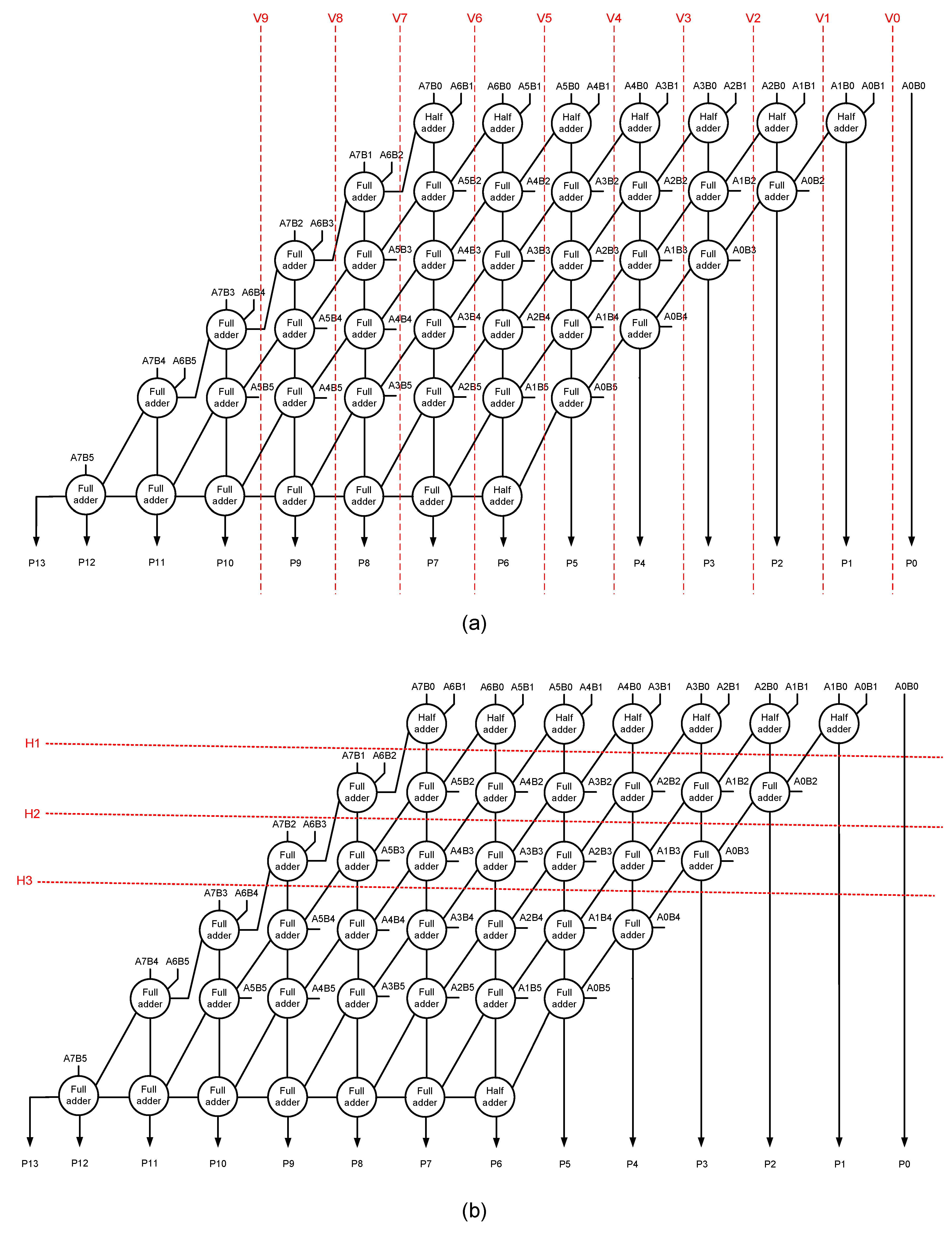
An accurate array multiplier can be transformed into an approximate array multiplier by introducing vertical or horizontal cuts in the carry-save adder [15]. Figure 2a shows some example vertical cuts, and Figure 2b shows a few examples of horizontal cuts.

For ease of reference, the vertical cuts are referred to as V0 to V9 in Figure 2a, and the horizontal cuts are referred to as H1 to H3 in Figure 2b. Subsequent to a vertical cut, the circuit portion present on the right side of the cut would be eliminated, and some input and output assignments can be made within the multiplier. On the other hand, subsequent to a horizontal cut, the circuit portion present above the cut would be eliminated and some input and output assignments can be incorporated in the multiplier.

In general, when a low-order vertical cut is introduced in an accurate array multiplier, the less significant partial product(s) would be eliminated first, whereas a low-order horizontal cut would chop off some significant partial products straightaway. For example, V1 in Figure 2a would eliminate only three less significant partial products i.e., A1B0, A0B1, and A0B0 besides a half adder, whereas H1 in Figure 2b would eliminate 15 partial products including some significant partial products such as A7B1, A6B2, A7B0, A6B1, etc., and 7 half adders. Therefore, a horizontal cut would have a greater impact than a vertical cut. Given this, vertical cuts are preferable over horizontal cuts to achieve a graded approximation. Nevertheless, in Section 5, we shall portray the effects of V0 to V9 and H1 to H3 on an example image corresponding to an image denoising application, which will validate our preference for vertical cuts over horizontal cuts in an accurate array multiplier to derive efficient approximate array multiplier(s).

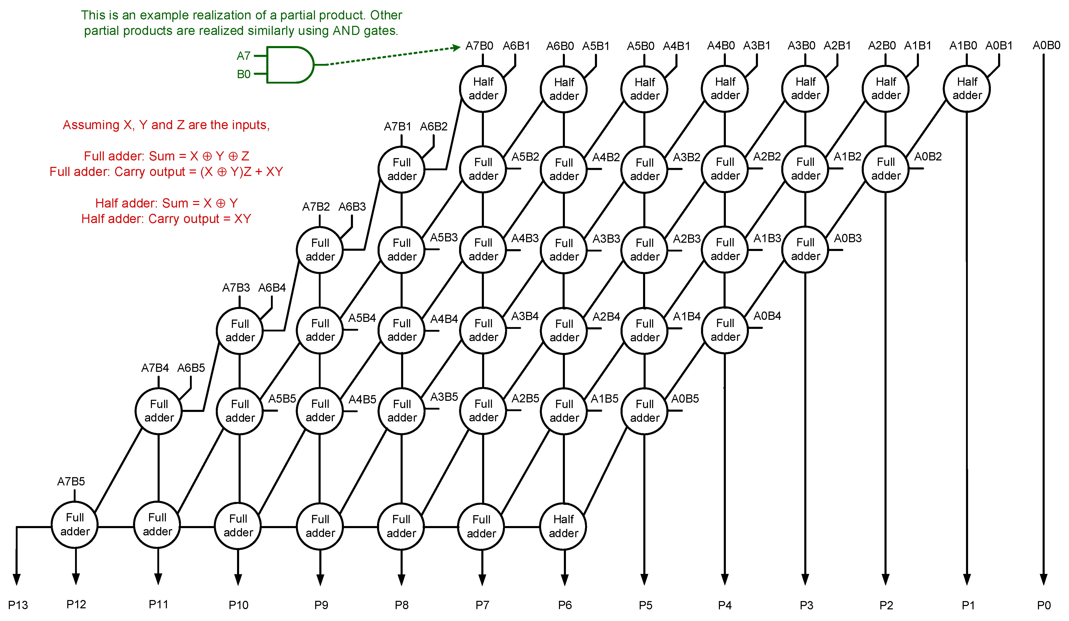
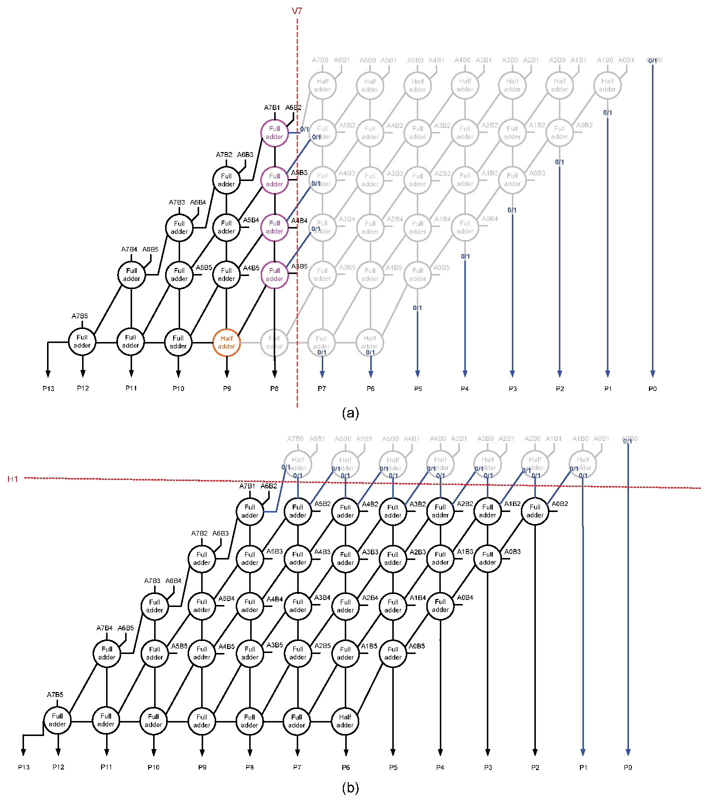
For clarity, we portray the consequence of a vertical cut V7 and a horizontal cut H1 on the accurate array multiplier (shown in Figure 1) through Figure 3a,b respectively. Subsequent to a vertical cut or a horizontal cut, the dangling internal inputs could be assigned a 0 or 1, which we refer to as internal input assignments. Likewise, the dangling (less significant) product bits could also be assigned a 0 or 1, which we refer to as output assignments. These are depicted in blue in Figure 3a,b.

Reference [15] suggested introducing vertical and horizontal cuts in an accurate array multiplier to obtain approximate (broken) array multipliers. With reference to Figure 2, the horizontal cut was suggested to be restricted to H2 and vertical cuts can be made as required. After making vertical and horizontal cuts, the dangling internal inputs and dangling product bits are assigned a constant 0. However, based on our experimentation with the digital image denoising application, horizontal cuts H2 and beyond are not found to be suitable due to exacerbated errors (discussed in Section 4), and the approximate array multiplier obtained via H1 and V7 cuts is structurally equivalent to an approximate array multiplier obtained via the V7 cut.

Yamamoto et al. [16] presented approximate array multipliers which are obtained by introducing only vertical cuts in an accurate array multiplier. After a vertical cut, binary 0 was given as an input to all the full adders present in a column that is adjacent to the vertical cut, and binary 0 was assigned to the less significant product bits whose logic have been eliminated. Henceforth, we refer to the approximate array multiplier (APAM) of [16] as APAM00_VN in general, wherein the first 0 implies the assignment of a 0 input to all the full adders present in a column that is adjacent to the vertical cut, and the second 0 implies the assignment of a 0 to those product bits whose logic have been eliminated. V implies a vertical cut, and N denotes the order of the vertical cut. These definitions of V and N hold well for all the approximate array multipliers to be discussed in this work.

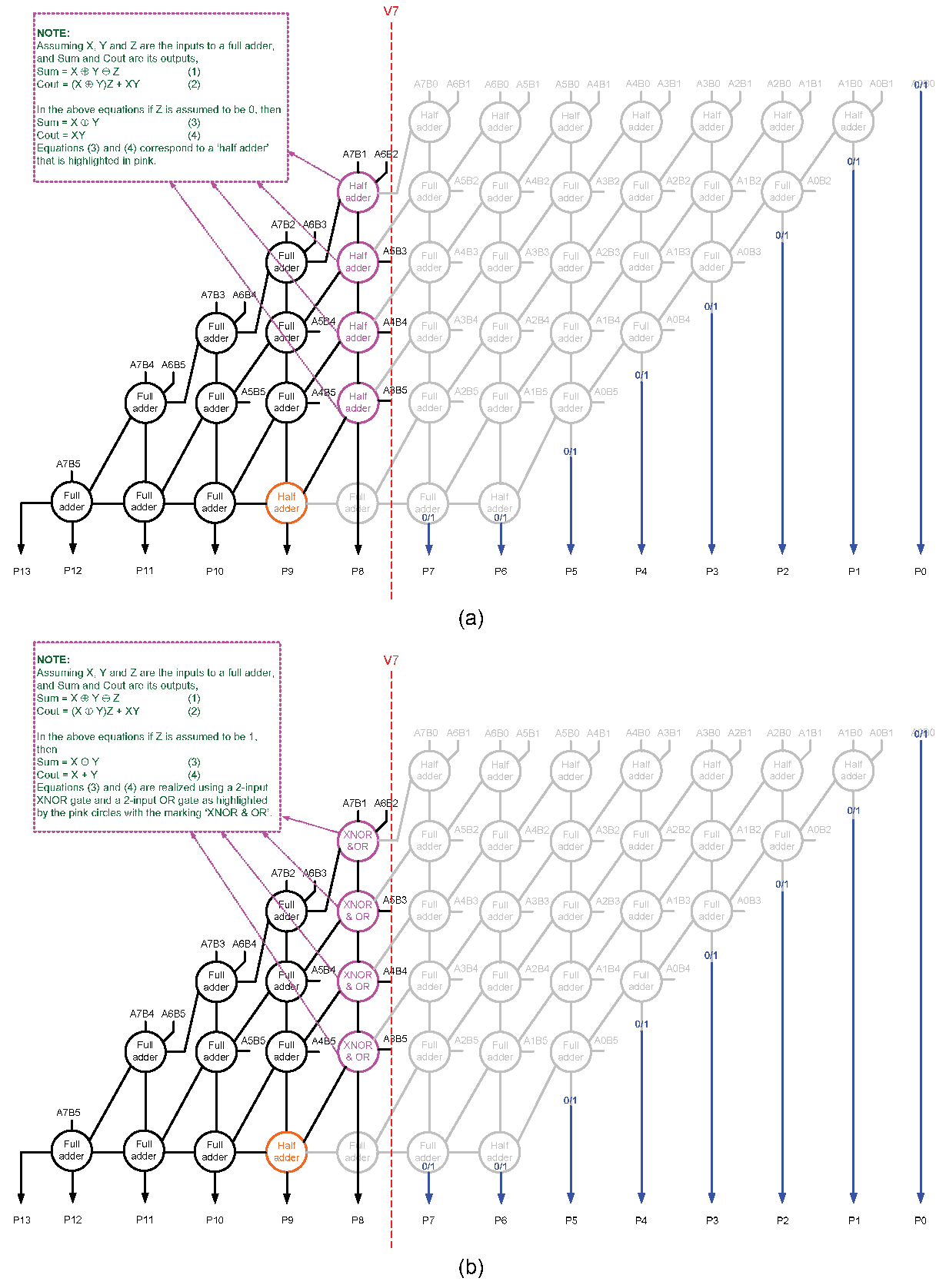
Subsequent to a vertical cut, it is possible to assign a 0 to the internal inputs and a 1 to the less significant product bits whose logic have been eliminated. Moreover, it is possible to assign a 1 to the internal inputs and a 0 to the less significant product bits whose logic have been eliminated. Further, it is possible to assign a 1 to the internal inputs and a 1 to the less significant product bits whose logic have been eliminated. Furthermore, it is possible to optimize the logic of some of the full adders or half adders after assigning a constant 0 or 1 input (post a vertical cut) prior to synthesis. For example, Figure 4a,b show how the full adders adjacent to a vertical cut V7, which are highlighted in pink in Figure 3a, can be optimized after assigning a constant 0 and 1 input. These possibilities were not considered in [16], and here we consider these possibilities as our proposition to derive an efficient approximate array multiplier.

We now discuss the acronyms which shall be used to refer to the proposed approximate array multipliers. Referring to Figure 2b, a proposed approximate array multiplier (PAAM) architecture featuring a vertical cut with a 0 assigned for the internal inputs and a 1 for the product bits whose logic have been eliminated shall be referred to as PAAM01_VN. A PAAM architecture featuring a vertical cut with a 1 assigned to the internal inputs and a 0 for the product bits whose logic have been eliminated shall be referred to as PAAM10_VN. A PAAM architecture featuring a vertical cut with a 1 assigned for the internal inputs and a 1 assigned for the product bits whose logic have been eliminated shall be referred to as PAAM11_VN.

Referring to Figure 2b, which shows the horizontal cuts, a PAAM architecture featuring a horizontal cut that assigns a 0 for the internal inputs and a 0 for the product bits whose logic have been eliminated shall be referred to as PAAM00_HN, and a PAAM architecture featuring a horizontal cut that assigns a 0 for the internal inputs and a 1 for the product bits whose logic have been eliminated shall be referred to as PAAM01_HN. H signifies a horizontal cut, and N denotes the order of the cut. Further, a PAAM architecture featuring a horizontal cut that assigns a 1 for the internal inputs and a 0 for the product bits whose logic have been eliminated shall be referred to as PAAM10_HN, and a PAAM architecture featuring a horizontal cut that assigns a 1 for the internal inputs and a 1 for the product bits whose logic have been eliminated shall be referred to as PAAM11_HN.

4. Error Parameters of Approximate Array Multipliers

Before analyzing the impact of different approximate array multipliers on a practical application (here, digital image denoising), information about their error parameters shall be provided to aid with further discussion.

Many error parameters are used in approximate computing such as absolute error magnitude (also called absolute error distance or simply absolute error), mean absolute error (also called mean error distance), worst-case error, root mean square error, etc. In this work, we consider two popular error parameters which are widely used, namely the mean absolute error (MAE) and the root mean square error (RMSE) for a comparative evaluation of the error attributes of approximate array multipliers. The RMSE is of particular interest among the different error parameters as it better captures the signal degradation of a digital signal processing application [17].

To calculate the error parameters of the approximate array multipliers, we developed Python models of the accurate multiplier and approximate array multipliers. For an 8×6 multiplier, there would be a total of 2¹⁴ i.e., 16384 distinct inputs, and all these inputs were considered to accurately estimate the error parameters of approximate array multipliers. For each approximate array multiplier, the modulus of the absolute difference between its generated product and the corresponding product of the accurate multiplier with respect to all the applied inputs were calculated. These differences were then averaged to calculate the MAE, given by Equation (1); the RMSE was calculated using Equation (2) [18]. In Equations (1) and (2), I represents the multiplicand which is of size 8 bits and J represents the multiplier which is of size 6 bits. Approx_Product(I,J) denotes the product of I and J computed by an approximate multiplier, and Accu_Product(I,J) denotes the product of I and J computed by the accurate multiplier. The difference between Approx_Product(I,J) and Accu_Product(I,J) may be positive, negative, or zero, depending upon the input applied.

$$\mathrm{MAE}=\frac{1}{2^{14}}{\displaystyle \sum }_{\mathrm{I}=0}^{2^8-1}{\displaystyle \sum }_{\mathrm{J}=0}^{2^6-1}|\mathrm{Approx}\_\mathrm{Product}\left(\mathrm{I},\mathrm{J}\right)-\mathrm{Accu}\_\mathrm{Product}\left(\mathrm{I},\mathrm{J}\right)|$$

(1)

$$\mathrm{RMSE}=\sqrt{\frac{1}{2^{14}}{\displaystyle \sum }_{\mathrm{I}=0}^{2^8-1}{\displaystyle \sum }_{\mathrm{J}=0}^{2^6-1}{\left(\mathrm{Approx}\_\mathrm{Product}\left(\mathrm{I},\mathrm{J}\right)-\mathrm{Accu}\_\mathrm{Product}\left(\mathrm{I},\mathrm{J}\right)\right)}^2}$$

(2)

Table 1. Error parameters of various approximate array multipliers obtained via different vertical and horizontal cuts.

Approximate Array Multiplier	MAE	RMSE
With Vertical Cuts
APAM_V0	0.25	0.50
PAAM_V0	0.75	0.87
APAM00_V1	1.25	1.94
PAAM01_V1	2.00	2.29
PAAM10_V1	2.88	3.12
PAAM11_V1	5.75	5.94
APAM00_V2	4.25	5.85
PAAM01_V2	4.19	4.87
PAAM10_V2	11.78	12.42
PAAM11_V2	18.75	19.18
APAM00_V3	12.25	15.76
PAAM01_V3	8.58	10.28
PAAM10_V3	35.76	37.10
PAAM11_V3	50.75	51.71
APAM00_V4	32.25	39.68
PAAM01_V4	18.53	23.15
PAAM10_V4	95.75	98.50
PAAM11_V4	126.75	128.84
APAM00_V5	80.25	95.70
PAAM01_V5	42.56	54.92
PAAM10_V5	175.85	183.32
PAAM11_V5	238.75	244.38
APAM00_V6	176.25	207.42
PAAM01_V6	92.01	119.93
PAAM10_V6	336.22	353.11
PAAM11_V6	462.77	475.50
APAM00_V7	368.25	430.74
PAAM01_V7	191.65	250.50
PAAM10_V7	657.04	692.77
PAAM11_V7	910.81	937.76
APAM00_V8	688.25	810.59
PAAM01_V8	355.34	463.45
APAM00_V9	1200.25	1436.50
PAAM01_V9	630.61	808.91
With Horizontal Cuts
PAAM00_H1	127.25	176.40
PAAM01_H1	125.78	174.24
PAAM10_H1	632.75	644.43
PAAM11_H1	635.75	647.38
PAAM00_H2	318.25	419.48
PAAM01_H2	313.10	414.19
PAAM10_H2	1201.75	1232.43
PAAM11_H2	1208.75	1239.26
PAAM00_H3	700.25	904.27
PAAM01_H3	687.38	892.70
PAAM10_H3	2339.75	2408.69
PAAM11_H3	2354.75	2423.26

shows the MAE and RMSE of 46 approximate array multipliers. We have considered V0 to V9 vertical cuts, and H1 to H3 horizontal cuts for the error calculation. V8 affects the quality of image denoising significantly, as will be discussed in the next section. Hence, with respect to V8 and V9 cuts, only APAM00_V8 and PAAM01_V8, and APAM00_V9, and PAAM01_V9 were considered for the error calculation since PAAM10_VN and PAAM11_VN architectures perform poorly even for a V7 cut. Also, since H3 affects the quality of image denoising considerably, which will be discussed in the next section, horizontal cuts beyond H3 were not considered for the error calculation. Further, the accurate (array) multiplier does not have any error and hence it is omitted from Table 1. Referring to Figure 2a, based on V0, the partial product A0B0 alone would be eliminated and there is no need for any internal input assignment. The least significant product bit P0 can alone be assigned a constant 0 or 1 after the V0 cut, which are referred to as APAM_V0 and PAAM_V0 respectively in Table 1.

Three general observations can be made from Table 1. First, as the order of a vertical cut or a horizontal cut increases, the error parameters increase owing to an increase in the approximation. Second, the approximate array multipliers obtained through horizontal cuts have greater MAE and RMSE compared to the approximate array multipliers obtained through vertical cuts. For example, approximate array multipliers obtained through the H3 cut have greater MAE and RMSE compared to the approximate array multipliers obtained through the V7 cut. Third, the PAAM01_VN architecture features lesser MAE and RMSE compared to APAM00_VN, PAAM10_VN, and PAAM11_VN architectures. For example, PAAM01_V7 reports reductions in MAE by 48%, 70.8%, and 79% compared to APAM00_V7, PAAM10_V7, and PAAM11_V7 respectively, and respective reductions in RMSE by 41.8%, 63.8%, and 73.3%.

Among the approximate array multiplier architectures obtained through vertical cuts, the error parameters of PAAM11_VN are relatively greater compared to its counterparts. In PAAM11_VN, constant 1 inputs are given internally and a constant 1 is assigned to those product bits whose logic were eliminated. Therefore, the PAAM11_VN architecture may likely cause an over-approximation for many inputs by exceeding the accurate product, and so PAAM11_VN has greater MAE and RMSE compared to its counterparts.

Overall, from Table 1, the PAAM01_VN architecture looks promising compared to the other architectures. Nevertheless, to confirm its utility, we consider digital image denoising as a practical application and analyze the impact of various approximate array multipliers in the next section.

5. Digital Image Denoising Application

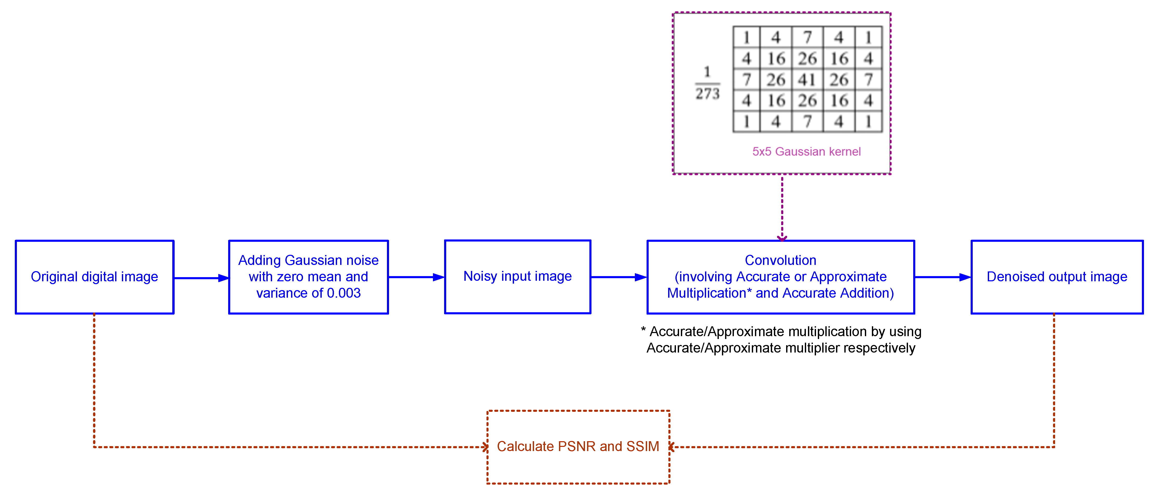
In this work, digital image denoising is considered as a practical application to evaluate and compare the performance of accurate and approximate array multipliers. The addition of noise to an original digital image and the subsequent image denoising process is illustrated through a block diagram in Figure 5. A random Gaussian noise with zero mean and a constant variance of 0.003 is added to an original image to create a noisy image. A 5 × 5 Gaussian low-pass filtering is then performed on the noisy image that is input by using accurate and approximate array multipliers individually to retrieve the corresponding denoised images.

A 5 × 5 Gaussian kernel [19], shown in Figure 5, is convolved with the noisy image for the denoising application, resulting in Equation (3). The filtering operation is performed as follows. Considering a pixel corresponding to the coordinate (x, y), the denoised pixel value at location (x, y) can be represented using Equation (3). In Equation (3), the × operator signifies approximate multiplication when using an approximate multiplier, and accurate multiplication when using the accurate multiplier. For edge pixels, the neighbors outside the scope of the image are used in the calculation through zero padding. All the addition operations and the division by 273 in equation (3) are performed accurately. A division by 273 is required for normalization since the sum of all the integer kernel coefficient values shown in Figure 5 is 273.

The gray values of the pixels correspond to a “multiplicand” which can be represented by 8 bits since the gray values vary from 0 to 255. The “multiplier” is used to represent the positive integer coefficients corresponding to the kernel shown in Figure 5. The maximum possible value of this coefficient being 41, it can be represented in binary using 6 bits as 101001. Given these, an 8×6 multiplier is sufficient for the digital image denoising application.

$$\begin{array}{cc}\hfill Denoised\left(x,y\right)=& \frac{1}{273}(Noisy\left(x-2,y-2\right)\times 1+Noisy\left(x-1,y-2\right)\times 4\hfill \\ \hfill & +Noisy\left(x,y-2\right)\times 7+Noisy\left(x+1,y-2\right)\times 4\hfill \\ \hfill & +Noisy\left(x+2,y-2\right)\times 1+Noisy\left(x-2,y-1\right)\times 4\hfill \\ \hfill & +Noisy\left(x-1,y-1\right)\times 16+Noisy\left(x,y-1\right)\times 26\hfill \\ \hfill & +Noisy\left(x+1,y-1\right)\times 16+Noisy\left(x+2,y-1\right)\times 4\hfill \\ \hfill & +Noisy\left(x-2,y\right)\times 7+Noisy\left(x-1,y\right)\times 26\hfill \\ \hfill & +Noisy\left(x,y\right)\times 41+Noisy\left(x+1,y\right)\times 26\hfill \\ \hfill & +Noisy\left(x+2,y\right)\times 7+Noisy\left(x-2,y+1\right)\times 4\hfill \\ \hfill & +Noisy\left(x-1,y+1\right)\times 16+Noisy\left(x,y+1\right)\times 26\hfill \\ \hfill & +Noisy\left(x+1,y+1\right)\times 16+Noisy\left(x+2,y+1\right)\times 4\hfill \\ \hfill & +Noisy\left(x-2,y+2\right)\times 1+Noisy\left(x-1,y+2\right)\times 4\hfill \\ \hfill & +Noisy\left(x,y+2\right)\times 7+Noisy\left(x+1,y+2\right)\times 4\hfill \\ \hfill & +Noisy\left(x+2,y+2\right)\times 1)\hfill \end{array}$$

(3)

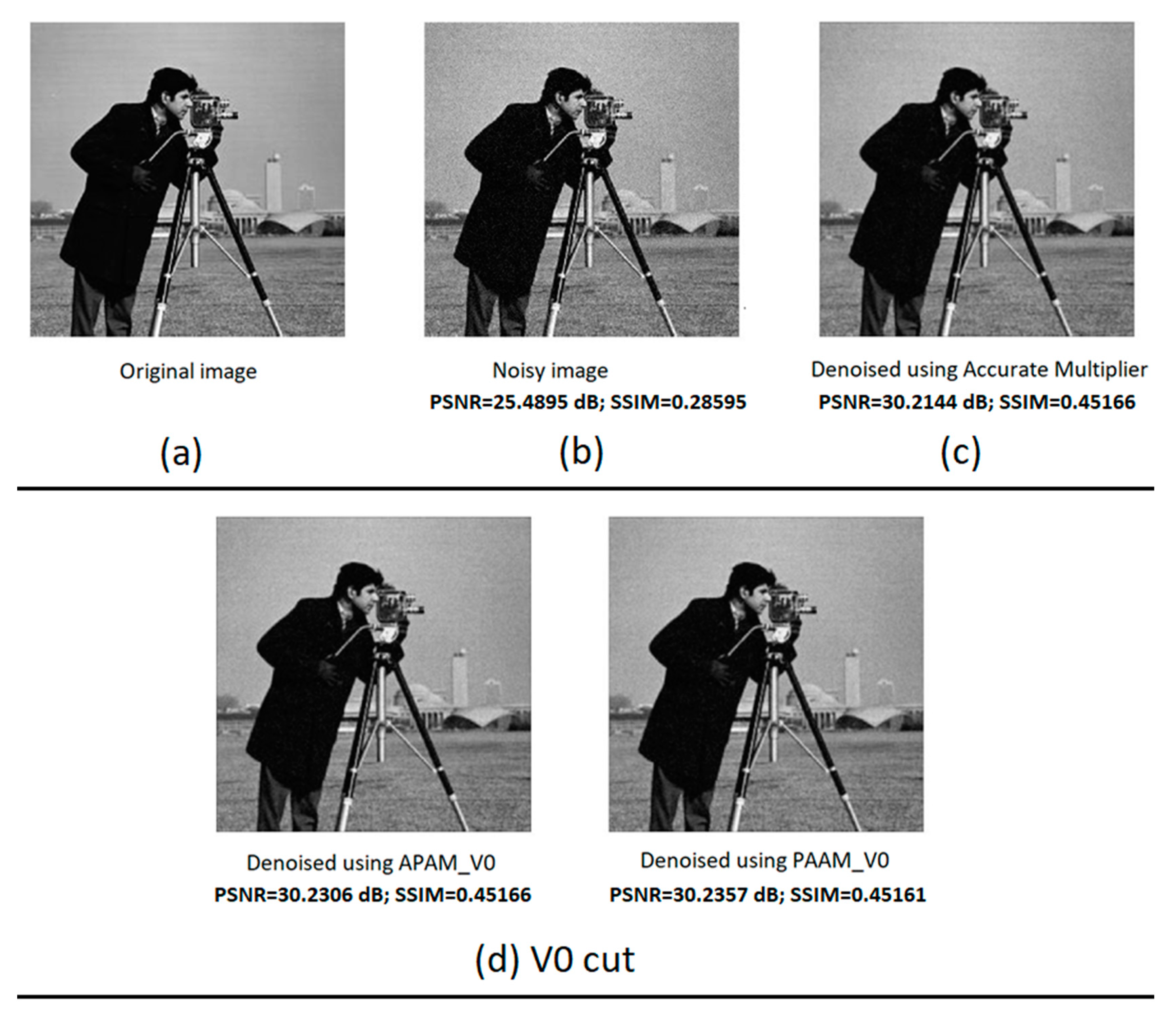
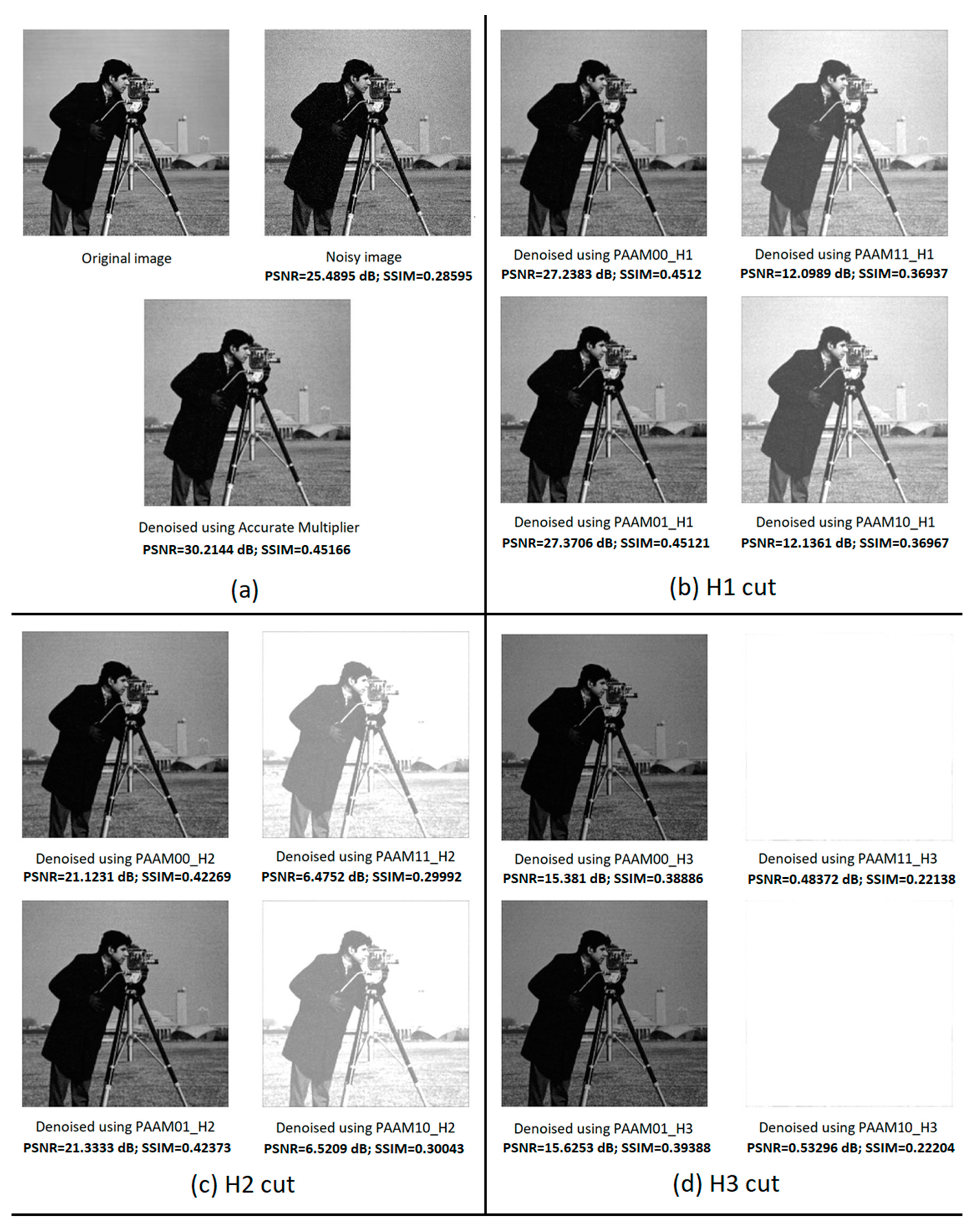
An original digital image (cameraman) with a grayscale resolution of 8 bits and a spatial resolution of 512 × 512 was considered for experimentation. The original noise, a noisy image resulting from the addition of the Gaussian noise, and the denoised image obtained through low-pass filtering by involving accurate multiplication are shown in Figure 6a–c respectively. Figure 6d shows the denoised images obtained through low-pass filtering by performing approximate multiplications by using approximate array multipliers APAM_V0 and PAAM_V0, which result from the V0 vertical cut.

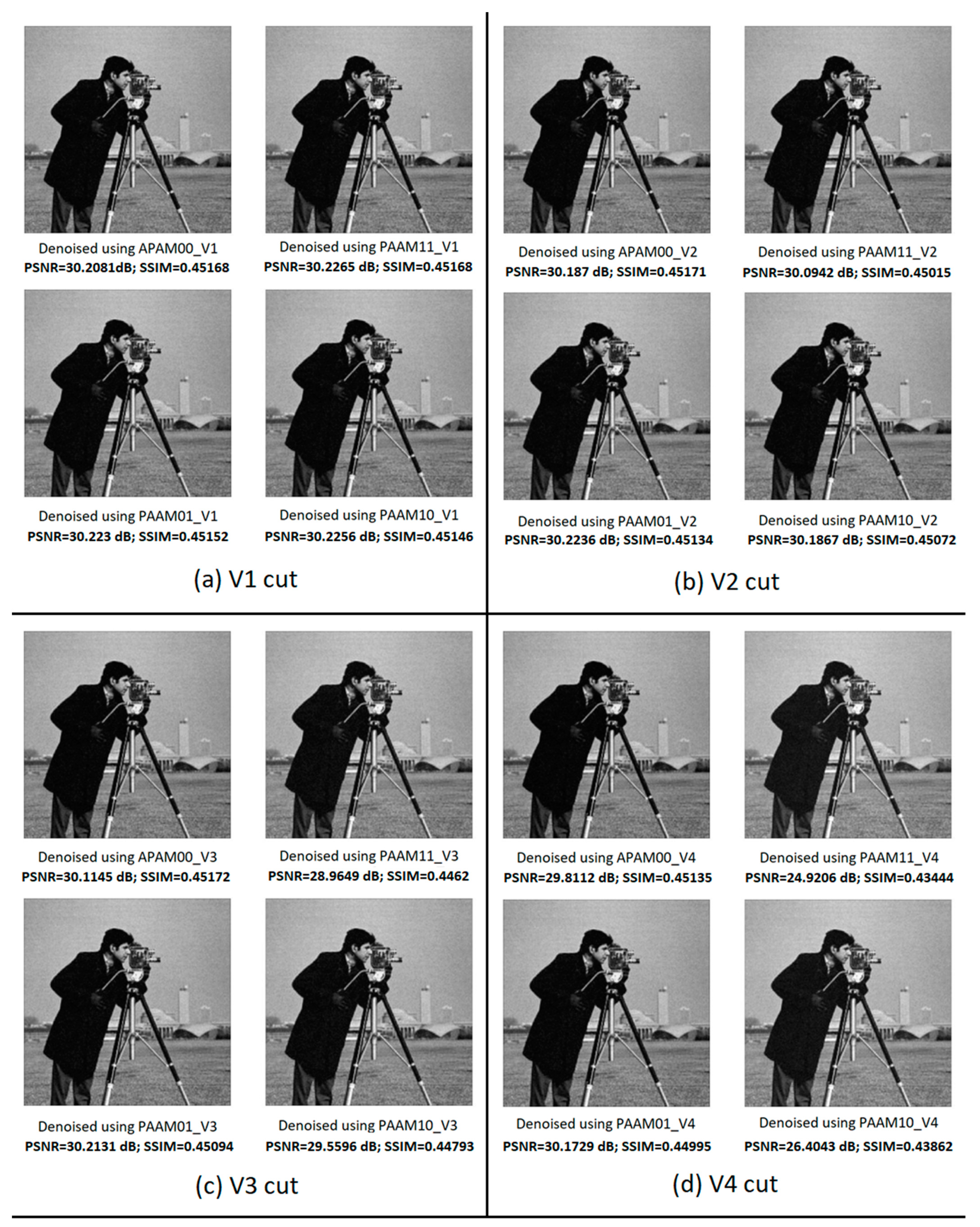
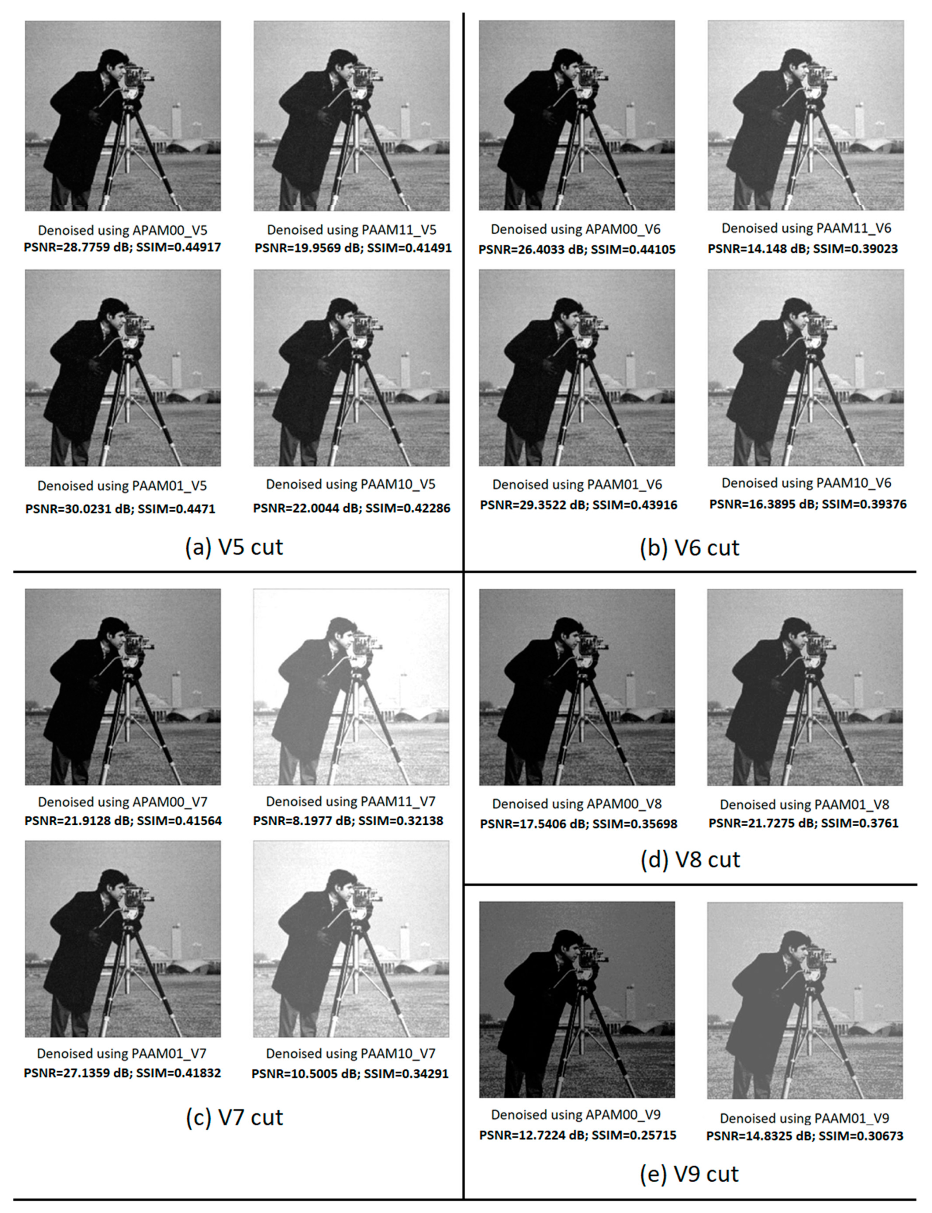
Figure 7 shows the denoised images obtained using approximate array multipliers resulting from vertical cuts V1 to V4, and Figure 8 shows the denoised images obtained using approximate array multipliers resulting from vertical cuts V5 to V9. Figure 9 shows the denoised images obtained using approximate array multipliers resulting from horizontal cuts H1 to H3.

The peak signal-to-noise ratio (PSNR) is a widely used qualitative figure-of-merit in digital signal processing [20]. The lesser the noise, the better the PSNR. Thus, a high value of PSNR, which is indicative of less noise/distortion, is preferable.

Besides PSNR, the structural similarity index metric (SSIM), is also used as a qualitative metric in digital image processing [20]. While PSNR quantifies the absolute error, SSIM quantifies the quality of a digital image in terms of the perceived change in structural information compared to an original (reference) image on a pixel-by-pixel basis. The value of SSIM ranges from 0 to 1, with 1 being the highest preferred value. Thus, similar to the PSNR, a high value of SSIM is preferable. We consider PSNR and SSIM as qualitative metrics for digital image processing in this work. We estimated PSNR and SSIM of the noisy image and the denoised images obtained using accurate and approximate array multipliers, and they are given in Figure 6, Figure 7, Figure 8 and Figure 9.

It may be noted that the lesser the approximation is introduced in a circuit, the lesser would be the savings in design metrics achievable compared to the accurate circuit [21]. Hence, it is important to strike a trade-off between the maximum approximation that can be incorporated in a circuit which would lead to maximum savings in the design metrics and the output quality (here, image quality) acceptable for a practical application.

From Figure 6, it is seen that APAM_V0 and PAAM_V0 yield nearly similar quality of denoised images as the accurate multiplier. However, APAM_V0 and PAAM_V0 are small approximations which would not help to significantly optimize the design metrics compared to the accurate multiplier, as will be seen in Section 6. Therefore, APAM_V0 and PAAM_V0 are not preferred approximations.

Referring to Figure 7 and Figure 8, among the various images shown, based on different vertical cuts, overall, the PAAM01_VN architecture yields better quality denoised images compared to its counterparts, which is evident from the corresponding PSNR and SSIM values. Up to the V3 cut, PAAM01_VN and APAM00_VN architectures yield nearly similar results but starting from the V4 cut, PAAM01_VN architecture is found to be preferable. This is mainly because APAM00_VN assigns a 0 to the less significant product bits and so any information contained in these product bits is completely lost. On the other hand, since PAAM01_VN assigns a 1 to the less significant product bits, the information contained in these bits is more than compensated for.

From Figure 6c, we note that the qualitative metrics of the image denoised using the accurate multiplier are: PSNR = 30.2144 dB; SSIM = 0.45166. From Figure 8c, we note that the qualitative metrics of the image denoised using PAAM01_V7 are: PSNR = 27.1359 dB; SSIM = 0.41832. Compared to Figure 6c, Figure 8c reports a 10.2% reduction in PSNR and a 7.4% reduction in SSIM. Nevertheless, visually, Figure 6c and Figure 8c look similar. Although PAAM_V0 and PAAM01_V1 up to PAAM01_V6 also yield good quality images (based on a comparison between Figure 6a,c, Figure 7a–d and Figure 8a,b), the maximum approximation is preferred in an approximate circuit that would help to significantly reduce the design metrics compared to an accurate circuit and simultaneously achieve an acceptable compromise on the output quality of a practical application. Given this, here, PAAM01_V7 represents a maximum approximation of the array multiplier that leads to a near similar output quality as the accurate array multiplier with considerably fewer logic gates, and hence PAAM01_V7 is preferable.

A further increase in the order of the vertical cut beyond V7 is not advisable since PAAM01_V8 and PAAM01_V9 result in a degradation of the image quality, as seen from Figure 8d,e, reporting much reduced PSNR and SSIM compared to the PSNR and SSIM of the accurately denoised image shown in Figure 6c. Since PAAM11_V7 and PAAM10_V7 result in poor quality images with relatively smaller PSNR and SSIM, PAAM11_VN and PAAM10_VN are not considered for analysis corresponding to V8 and V9 cuts in Figure 8d,e.

With respect to the images denoised using approximate array multipliers, derived from horizontal cuts, as shown in Figure 9, the H3 cut leads to a complete loss of the image as seen from Figure 9d. The drawback with horizontal cuts is that even a low order horizontal cut would eliminate some significant partial products straightaway whereas vertical cuts would progressively eliminate partial products starting from the least significant ones. From Figure 9b, it can be seen that even the H1 cut may not be acceptable since PAAM00_H1 and PAAM01_H1 based images appear darker than the accurately denoised image shown in Figure 9a. Moreover, H1 eliminates 7 half adders and 15 2-input AND gates and optimizes the logic of 7 full adders of the accurate array multiplier, as seen from Figure 3b, whereas V7 would eliminate more components i.e., 20 full adders and 8 half adders and optimize the logic of 5 full adders as seen from Figure 4a. Therefore, based on the error parameters given in Table 1 and the image processing results given in Figure 6, Figure 7, Figure 8 and Figure 9, approximate array multipliers obtained via vertical cuts are preferable, and here, in particular, PAAM01_V7 is preferable.

6. Implementation Results

An accurate array multiplier and 30 approximate array multipliers obtained via vertical cuts from V0 to V7 were described in Verilog hardware description language (HDL) at the gate-level and synthesized using a 32/28-nm CMOS standard digital cell library [22]. Since vertical cuts V8 and beyond were not found to be beneficial, as evident from the error parameters given in Table 1 and the denoised images shown in Figure 8d,e, these were omitted from the implementation. Also, since horizontal cuts were not found to be more beneficial than the vertical cuts, as evident from Table 1 and Figure 9, approximate array multipliers with horizontal cuts were also omitted from the implementation.

Synopsys tools were used for functional simulation, synthesis, and estimation of the design metrics such as critical path delay, total area (i.e., cells area plus interconnect area), and average total power dissipation. Synopsys Design Compiler was used for synthesis, VCS was used to perform functional simulation, and PrimeTime and PrimePower were used to estimate critical path delay and total power dissipation respectively. About a thousand random inputs were supplied to the multipliers through a common test bench at time intervals of 2.5 ns (400 MHz) to verify the functionalities, and the switching activity data gathered was used to estimate the average total power. A typical case process, voltage and temperature specification with a recommended supply voltage of 1.05 V and an operating junction temperature of 25 °C was used for the simulations. Wire loads were considered as a part of the simulations, and a fan-out of 4 drive strength was assigned to all the output ports (i.e., the product bits). The design metrics estimated are given in

Table 2. Design metrics of accurate and approximate array multipliers, estimated using a 32/28-nm complementary metal-oxide-semiconductor (CMOS) process.

Array Multiplier	Area (µm2)	Delay (ns)	Power (µW)
Accurate	383.07	1.75	135.7
APAM_V0 and PAAM_V0 architectures
APAM_V0	378.89	1.77	130.2
PAAM_V0	378.89	1.77	130.2
APAM00_VN architecture
APAM00_V1	367.47	1.76	127.6
APAM00_V2	349.94	1.75	121.8
APAM00_V3	323.09	1.71	108.4
APAM00_V4	297.04	1.71	94.6
APAM00_V5	245.40	1.59	74.9
APAM00_V6	184.40	1.58	56.2
APAM00_V7	135.77	1.26	32.8
PAAM01_VN architecture
PAAM01_V1	367.47	1.76	127.6
PAAM01_V2	349.94	1.75	121.8
PAAM01_V3	323.09	1.71	108.4
PAAM01_V4	297.04	1.71	94.6
PAAM01_V5	245.40	1.59	74.9
PAAM01_V6	184.40	1.58	56.2
PAAM01_V7	135.77	1.26	32.8
PAAM10_VN architecture
PAAM10_V1	368.88	1.77	126.8
PAAM10_V2	357.16	1.72	127.0
PAAM10_V3	349.02	1.78	121.2
PAAM10_V4	302.48	1.73	105.5
PAAM10_V5	253.17	1.63	80.6
PAAM10_V6	187.57	1.47	68.4
PAAM10_V7	135.60	1.19	44.3
PAAM11_VN architecture
PAAM11_V1	368.88	1.77	126.8
PAAM11_V2	357.16	1.72	127.0
PAAM11_V3	349.02	1.78	121.2
PAAM11_V4	302.48	1.73	105.5
PAAM11_V5	253.17	1.63	80.6
PAAM11_V6	187.57	1.47	68.4
PAAM11_V7	135.60	1.19	44.3

.

It can be seen from Table 2 that as the approximation is increased from V0 to V7, the areas of the approximate array multipliers decrease, and consequently their power dissipation decreases. Depending upon the critical path exercised, the maximum delay of an approximate array multiplier remains the same as the accurate array multiplier or is reduced.

In Table 2, APAM00_VN and PAAM01_VN architectures have the same design metrics, and PAAM10_VN and PAAM11_VN architectures also have the same design metrics. This is because, between these two architectural pairs, the only difference is the assignment of a constant 0 or 1 to some less significant product bits while the rest of the multiplier logic remains the same. The assignment of a constant 0 or 1 to a product bit is physically realized using a TIEL (tie-to-low) standard cell or a TIEH (tie-to-high) standard cell and both these cells have the same physical characteristics [22]. Hence, APAM_V0 and PAAM_V0, APAM00_VN and PAAM01_VN, and PAAM10_VN and PAAM11_VN architectures yield the same design metrics.

The design metrics of PAAM10_VN and PAAM11_VN are shown in Table 2 just for a comparison, given that Section 4 and Section 5 have already made clear that the PAAM01_VN architecture is preferable to its counterparts, based on the error metrics and the image denoising results. In Table 2, APAM00_VN and PAAM01_VN architectures exhibit reduced critical path delay compared to the accurate array multiplier starting from the V3 cut. However, it is important to choose a maximum approximation to gain maximum savings in the design metrics whilst ensuring an acceptable output quality. Based on the error parameters provided in Section 4 and the digital image denoising results presented in Section 5, it was inferred that PAAM01_V7 is preferable. Given this, from Table 2, it is noted that PAAM01_V7 achieves significant reductions in design metrics compared to the accurate array multiplier viz. 64.6% reduction in area, 28% reduction in critical path delay, and 75.8% reduction in power. The trade-off being that the denoised image obtained using PAAM01_V7 (Figure 8c) has moderately lesser PSNR and SSIM compared to the denoised image obtained using the accurate multiplier (Figure 6c). However, there is no significant visual difference between Figure 6c (image denoised using the accurate multiplier) and Figure 8c (image denoised using PAAM01_V7).

For analysis, we also implemented PAAM01_H1 since the digital image denoised using PAAM01_H1 shown in Figure 9b has almost the same PSNR as the digital image denoised using PAAM01_V7, which is shown in Figure 8c, and their error parameters are also somewhat comparable. In the case of PAAM01_H1 shown in Figure 3b, two constant 0 inputs are given to the full adders present in the second row, except for the left-most full adder, and these would get eliminated leaving just the corresponding partial products which are directly given as inputs to the full adders. As a consequence, in the third row, except for the two left-most full adders, the remaining full adders would reduce to half adders. After implementation, the area, delay, and power of PAAM01_H1 are estimated to be 269.68 µm², 1.41ns, and 82.8 µW respectively. Compared to PAAM01_H1, PAAM01_V7 has 10.6% less critical path delay, requires 49.7% less area, and dissipates 51.8% less power.

Further, we described an 8×6 multiplication accurately using the multiplication operator in Verilog HDL and auto-synthesized a high-speed accurate multiplier using Synopsys Design Compiler and estimated its design metrics which are as follows: critical path delay, 1.52 ns; area, 349.81 µm²; and power, 107 µW. In comparison with the high-speed accurate multiplier, PAAM01_V7 reports a 17.1% reduction in critical path delay, 61.2% reduction in area, and 69.3% reduction in power.

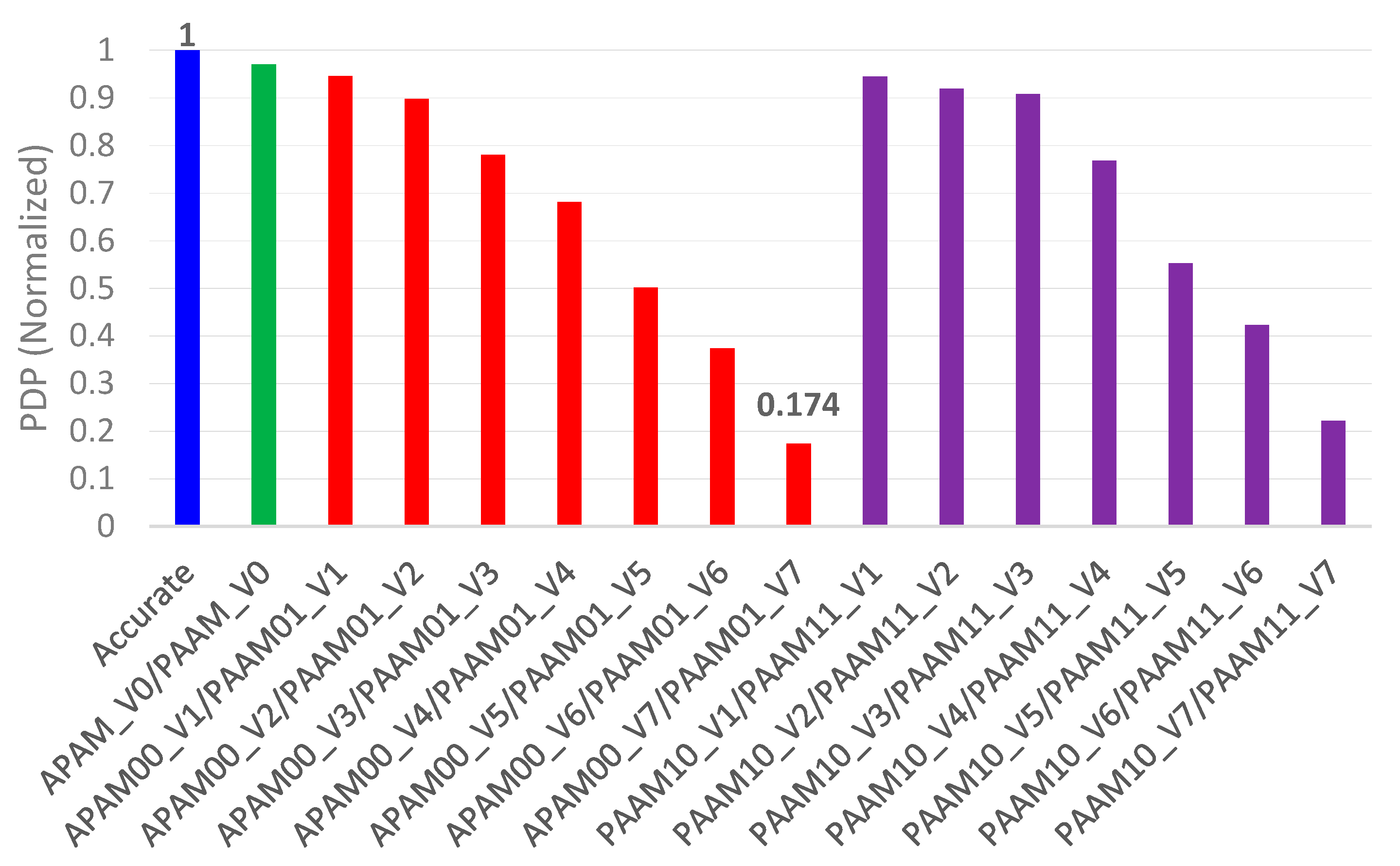
We also calculated the power-delay product (PDP), that is representative of energy, which is a popular figure-of-merit for low power in VLSI designs. Since power and (maximum propagation) delay are desirable to be less, the PDP is also desired to be less. Hence, the lesser the PDP, the better is the energy efficiency of a digital logic design. The absolute PDP values of accurate and approximate array multipliers were calculated and then normalized, which are plotted in Figure 10. To perform the normalization, the highest PDP value is considered as the baseline and this was used to divide the PDP values of all the array multipliers.

It was mentioned previously that APAM_V0 and PAAM_V0, APAM00_VN and PAAM01_VN, and PAAM10_VN and PAAM11_VN architectural pairs have the same design metrics. Given this, in Figure 10, the normalized PDP of the accurate array multiplier is shown by the blue bar, the normalized PDP of APAM_V0 and PAAM_V0 are shown in green, the normalized PDP of APAM00_VN and PAAM01_VN architectures are shown in red, and the normalized PDP of PAAM10_VN and PAAM11_VN architectures are shown in violet. It is seen from Figure 10 that, among the lot, APAM00_V7 and PAAM01_V7 have relatively lesser PDP since their power and delay metrics are better optimized, as evident from Table 2. However, PAAM01_V7 has less MAE and RMSE compared to APAM00_V7, as noted from Table 1, and the former enables a better image quality compared to the latter which is substantiated by the PSNR and SSIM values given in Figure 8c. Hence, PAAM01_V7 is preferable. In terms of the PDP, PAAM01_V7 is 82.6% better optimized compared to the accurate array multiplier, and 74.6% better optimized compared to the auto-synthesized high-speed accurate multiplier.

7. Conclusions

We explored ways of systematically approximating an accurate array multiplier by progressively introducing vertical or horizontal cuts and assigned new combinations of constant 0 and/or 1 to the dangling internal inputs and dangling product bits. Subsequent to a vertical or a horizontal cut in an accurate array multiplier, and after assigning some constant internal inputs and outputs, we also suggest optimizing the logic prior to synthesis. In general, vertical cuts are preferable to horizontal cuts to achieve a graded approximation and to derive an efficient approximate array multiplier. The proposed approximation techniques are generic and can be applied to a multiplier of any size commensurate with a target application.

Besides an existing approximate array multiplier architecture (APAM00_VN), many approximate array multiplier architectures were proposed and presented, namely PAAM01_VN, PAAM10_VN, PAAM11_VN, PAAM00_HN, PAAM01_HN, PAAM10_HN, and PAAM11_HN, and their efficacy were analyzed. Among these, PAAM01_VN, which is obtained by making a vertical cut in an accurate array multiplier and assigning a constant 0 for the dangling internal inputs and a constant 1 for the dangling product bits, is found to be efficient, which is substantiated by the error parameters estimated.

The utility of existing and proposed approximate array multipliers for a practical digital image denoising application was also analyzed. Based on the error parameters and the denoised digital images obtained, PAAM01_V7, which corresponds to a proposed approximate multiplier architecture viz. PAAM01_VN is found to be preferable. For an 8×6 multiplication, PAAM01_V7 achieves a 64.6% reduction in area, 28% reduction in critical path delay, 75.8% reduction in power, and 82.6% reduction in PDP compared to the accurate array multiplier whilst ensuring an acceptable image quality.