1. Introduction
The increase in Android’s popularity worldwide has made it a continuous target for malware authors. The volume of malware targeting Android has continued to grow in the last few years [
1,
2]. Android has been attacked by numerous malware families aimed at infecting mobile devices and turning them into bots. These bots become parts of larger botnets that are usually under the control of a malicious user or group of users known as botmasters. The Android botnets may be used to launch various types of attacks such as distributed denial of service (DDoS) attacks, phishing, click fraud, theft of credit card details or other credentials, generation and distribution of spam, etc. Nowadays, malicious Android botnets have become a serious threat. Additionally, their increasing use of sophisticated evasive techniques such as self-protection or multi-staged payload execution [
3], calls for more effective approaches to detect them.
The Chamois malware family [
3,
4,
5], which was discovered on Google Play in August 2016 is one example of the emerging sophisticated Android botnet threats. By March 2018, Chamois had infected over 20 million devices, which were commandeered into a botnet that received instructions from a remote command and control server [
5]. The botnet was used to serve malicious advertisements and to direct victims to premiums Short Message Service (SMS) scams. The early version of Chamois disguised as benign apps that tricked users into downloading it on their devices, and this was detected and almost completely eradicated by the Android security team. Later versions of Chamois appeared which were distributed by tricking developers and device manufacturers into incorporating the botnet code directly into their apps. Chamois was sold to developers as a legitimate software development kit, and to the device manufacturers as a mobile payment solution [
5].
The emergence of evasive and technically complex families like Chamois has driven interest in adopting machine learning based techniques as a means to improve existing detection systems. In the past few years, several works have investigated traditional machine learning techniques such as Support Vector Machines (SVM), Random Forest, Decision Trees, etc., for Android botnet detection. Some of the more recent machine learning based Android botnet detection work, such as ref. [
6] and ref. [
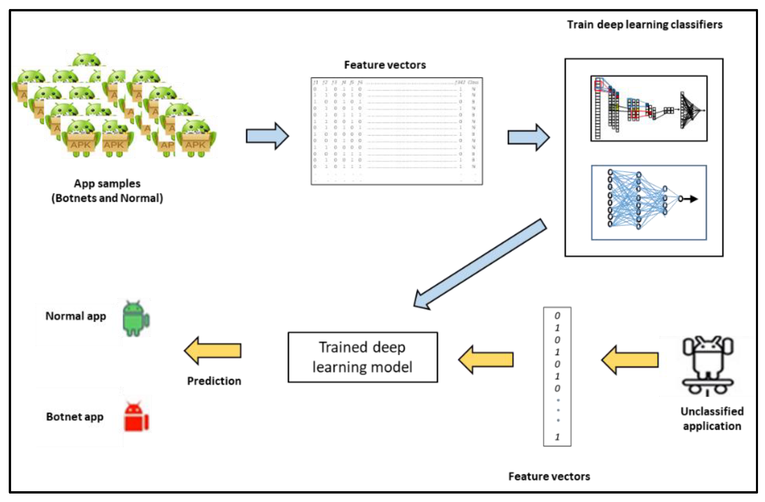
7] have focused on deep learning. Nevertheless, empirical studies that extensively investigate various deep learning techniques to provide insight into their relative performance for Android botnet detection are currently lacking. Hence, in this paper, we present a comparative analysis of deep learning models for Android botnet detection using the publicly available ISCX botnet dataset. Our approach is based on classification of unknown applications into ‘clean’ or ‘botnet’ using 342 static features extracted from the apps. We evaluate the performance of several deep learning models on 6802 apps consisting of 1929 botnet apps from the ISCX botnet dataset. The models investigated include Convolutional Neural Networks (CNN), Dense Neural Networks (DNN), Gated Recurrent Units (GRU), Long Short-Term Memory (LSTM), as well as more complex networks like CNN-LSTM and CNN-GRU.
The rest of the paper is organized as follows:
Section 2 contains related works.
Section 3 gives an overview of the overall system for deep learning-based Android botnet detection, while
Section 4 provides brief background discussions of the deep learning models that were built for this study.
Section 5 discusses the methodology and experimental approach, while
Section 6 presents the results and discussion of results. Finally, the conclusions and future work are outlined in
Section 7.
2. Related Work
Kadir et al. in their paper [
8], studied several families of Android botnets aiming to gain a better understanding of the botnets and their communication characteristics. They presented a deep analysis of the Command and Control channels and built-in URLs of the Android botnets. They provided insights into each malicious infrastructure underlying the families, and uncovered the relationships between the botnet families by using a combination of static and dynamic analysis with visualization. From their work, the ISCX Android botnet dataset consisting of 1929 samples from 14 Android botnet families emerged. Since then, several works on Android botnet detection have been based on the dataset which is available from ref. [
9].
Anwar et al. [
10] proposed a mobile botnet detection method based on static features. They combined permissions, MD5 signatures, broadcast receivers, and background services to obtain a comprehensive set of features. They then utilized these features to implement machine learning based classifiers to detect mobile botnets. Having performed experiments using 1400 botnet applications of the ISCX dataset, combined with an extra 1400 benign applications, they recorded an accuracy of 95.1%, a recall of 0.827, and a precision of 0.97 as their best results.
Android Botnet Identification System (ABIS) was proposed in [
11] to detect Android botnets. The method is based on static and dynamic features consisting of API calls, permissions, and network traffic. ABIS was evaluated with several machine learning techniques. In the end, Random Forest was found to perform better than the other algorithms by achieving 0.972 precision and 0.96 recall.
In ref. [
12], machine learning was used to detect Android botnets using permissions and their protection levels as features. Initially, 138 features were utilized and then increased to 145 after protection levels were added as novel features. In total, four machine learning models (i.e., Random Forest, multilayer perceptron (MLP), Decision Trees, and Naive Bayes) were evaluated on 3270 applications containing 1635 benign and 1635 botnets from the ISCX dataset. Random Forest was found to have the best results yielding 97.3% accuracy, 0.987 recall, and 0.985 precision. The authors of [
13] also utilized only the ‘requested permissions’ as features and applied Information Gain to reduce the features and select the most significant requested permissions. They evaluated their approach using Decision Trees, Naive Bayes, and Random Forest. In their experiments, Random Forest performed best, with an accuracy of 94.6% and false positive rate of 0.099%.
Karim et al. in [
14], proposed DeDroid, a static analysis approach to investigate properties that are specific to botnets that can be used in the detection of mobile botnets. in their approach, ‘critical features’ were first identified by observing the coding behavior of a few known malware binaries that possess Command and Control features. These ‘critical features’ were then compared with features of malicious applications from Drebin dataset [
15]. The comparison with ‘critical features’ suggested that 35% of the malicious applications in the Drebin dataset could be classed as botnets. However, according to their study, a closer examination confirmed 90% of the apps as botnets.
Jadhav et al. [
16], present a cloud-based Android botnet detection system that leverages dynamic analysis by using a virtual environment with cluster analysis. The toolchain for the dynamic analysis process is composed of strace, netflow, logcat, sysdump, and tcpdump within the botnet detection system. However, in the paper there were no experimental results provided to evaluate the effectiveness of the proposed cloud-based solution. Moreover, the virtual environment can easily be evaded by the botnets using different fingerprinting techniques. In addition, being a dynamic-analysis based approach, the systems effectiveness could be degraded by the lack of complete code coverage [
17,
18].
In ref. [
19], a method was proposed by Bernardeschia et al. to identify Android botnets through model checking. Model checking is an automated technique used in verifying finite state systems. This is achieved by checking whether a structure representing a system satisfies a temporal logic formula describing their expected behavior. In particular, static analysis is used to derive a set of finite state automata from the Java byte code that represents approximate information about the run-time behavior of an app. Afterwards, the botnet malicious behavior is formulated using temporal logic formulae [
20]; then by adopting a model checker, it can be automatically checked whether the code is malicious and identify where the botnet code is located within the application. These properties are checked using the CAAL (Concurrency Workbench, Aalborg Edition) [
21] formal verification environment. The authors evaluated their approach on 96 samples from the Rootsmart botnet family, 28 samples from the Tigerbot botnet family, in addition to 1000 clean samples. The results obtained on the 1124 app samples showed perfect (100%) accuracy, precision, and recall.
Alothman and Rattadilok [
22] proposed a source code mining approach based on reverse engineering and text mining techniques to identify Android botnet applications. Dex2Jar was used to reverse engineer the Android apps to Java source code. Natural Language Processing techniques were applied to the obtained Java source code. They also evaluated a ‘source code metrics (SCM)’ approach of classifying the apps into ‘botnet’ or ‘clean’. In the SCM approach, statistical measures, such as total number of code lines, code to comment ratio, etc., were extracted from the source code and the metrics were used as features for training machine learning classifiers. The Java source code was extracted from 9 apps from 9 ISCX botnet families, as well as 12 normal apps. The TextToWordVector filter within WEKA (Waikato Environment for Knowledge Analysis), together with TF-IDF, was then applied to the code. They also applied WEKA’s StringToWordVector with TF-IDF filter while varying the numbers of the ‘words to keep’ parameter. SubSetEval feature selection method was used to reduce the features. The features were applied to Naive Bayes, KNN, J48, SVM, and Random Forest algorithms, were KNN obtained the best performance.
In ref. [
23], a real-time signature-based detection system is proposed to combat SMS botnets, by first applying pattern-matching detection approaches for incoming and outgoing SMS text messages. In the second step, rule-based techniques are used to label unknown SMS messages as suspicious or normal. Their method was evaluated with over 12,000 test messages, where all 747 malicious SMS messages were detected in the dataset. However, the system produced some false positives where 349 SMS messages were flagged as suspicious. In ref. [
24], a botnet detection technique called ‘Logdog’ is proposed for mobile devices using log analysis. The approach relies on analyzing the logs of mobile devices to find evidence of botnet activities. Logdog writes logcat messages to a text file in the background while the Android user continues to use their device. The system targets HTTP botnets looking for events or series of events that indicate botnet activities and was tested manually on a botnet and a normal app.
In ref. [
6], Android botnet detection based on CNN and using permissions as features was proposed. In the proposed method, apps are represented as images that are constructed based on the co-occurrence of permissions used within the applications. The images were then used to train a CNN-based binary classifier. The binary classifier was evaluated using 5450 apps containing 1800 botnet apps from the ISCX dataset. They obtained an accuracy of 97.2%, with a recall of 0.96, precision of 0.955, and f-measure of 0.957. Similarly, ref. [
7] proposes an Android botnet detection approach based on CNN, where not only permissions were used as features but also API calls, Commands, Intents, and Extra Files. Unlike in ref. [
6], 1D CNN was used and the model was evaluated with the 1929 ISCX botnet apps and 4873 benign apps resulting in 98.9% accuracy, 0.978 recall, 0.983 precision, and 0.981 F1-score.
Different from the aforementioned earlier works, this paper aims to investigate the performance of several deep learning techniques to gain insight into their effectiveness in detecting Android botnets based on the extraction of 342 static features from the applications. To this end, we implemented CNN, DNN, LSTM, GRU, CNN-LSTM, and CNN-GRU models and evaluated the models using 1929 ISCX botnet apps and 4873 benign apps. The deep learning models developed in the study are discussed in
Section 4 and the results of the experiments with the models are presented in
Section 6.
5. Methodology and Experiments
In this section, we further detail our approach and outline the experiments undertaken to evaluate the deep learning models implemented in this paper. The models were developed in Python using the Keras library with TensorFlow backend. Other libraries utilized include Scikit Learn, Seaborn, Pandas, and Numpy. The experiments were performed on a Ubuntu Linux 16.04 64-bit Machine with 8GB RAM.
5.1. Problem Definition
Let A = {a1, a2, … an} be a set of applications where each ai is represented by a vector containing the values of n features (where n = 342). Let a = {f1, f2, f3, … fn, cl} where cl ∈ {botnet, normal} is the class label assigned to the app. Thus, A can be used to train a model to learn the behaviors of botnet and normal apps, respectively. The goal of a trained model is then to classify a given unlabeled app Aunknown = {f1, f2, f3, … fn, ?} by assigning a label cl, where cl ∈ {botnet, normal}.
5.2. Dataset Used for the Investigation
As mentioned earlier, the ISCX Android botnet dataset from [
9] was utilized for the experiments in this paper. This dataset contains 1929 botnet apps and has been employed in previous works including [
6,
7,
8,
10,
11,
12,
13,
22].
Table 3 shows the distribution of samples within the 14 different botnet families present in the dataset. To complement the ISCX dataset, we obtained 4873 clean from Google Play store. These apps were cross-checked for maliciousness using Virus Total (
https://www.virustotal.com (accessed on 20 December 2020)). Thus, a total of 6802 apps were used in our experiments.
5.3. Experiments to Evaluate the Deep Learning Techniques on the Android Dataset
In order to investigate the performance of the deep learning models, we performed several experiments with different configurations of the models to enable us observe the optimum performance that is possible with each model architecture. The models are designed to exploit the capabilities of the constituent neural network types as discussed in
Section 4. The following metrics are used in measuring the performance of the models: Accuracy, precision, recall, and F1-score. Given TP as true positives, FP as false positives, FN as false negatives, and TN as true negatives (all with respect to the botnet class), the metrics are defined as follows (taking the botnet class as positive):
Accuracy: the ratio between correctly predicted outcomes and the sum of all predictions expressed as:
Precision: All true positives divided by all positive predictions, i.e., was the model right when it predicted positive? Expressed as:
Recall: All true positives divided by all actual positives. That is, how many positives did the model identify out of all possible positives? Expressed as:
F1-score: This is the weighted average of precision and recall, given by:
All the results of the experiments are from 10-fold cross validation where the dataset is divided into 10 equal parts with 10% of the dataset held out for testing, while the models are trained from the remaining 90%. This is repeated until all of the 10 parts have been used for testing. The average of all 10 results is then taken to produce the final result. Additionally, during the training of all the deep learning models (for each fold), 10% of the training set was used for validation.
6. Results and Discussions
This section will present the results of investigating CNN-GRU, CNN-LSTM, CNN, and DNN models. Subsequently, a comparative performance evaluation of the models and how they measure against traditional machine learning models will be discussed. Finally, we will examine how these models have performed compared to results reported in previous works on Android botnet detection.
6.1. CNN-GRU Model Results
Here, we present the results obtained from CNN-GRU model where the configurations of both the CNN layer and the GRU layer were varied. A summary of the results is presented in
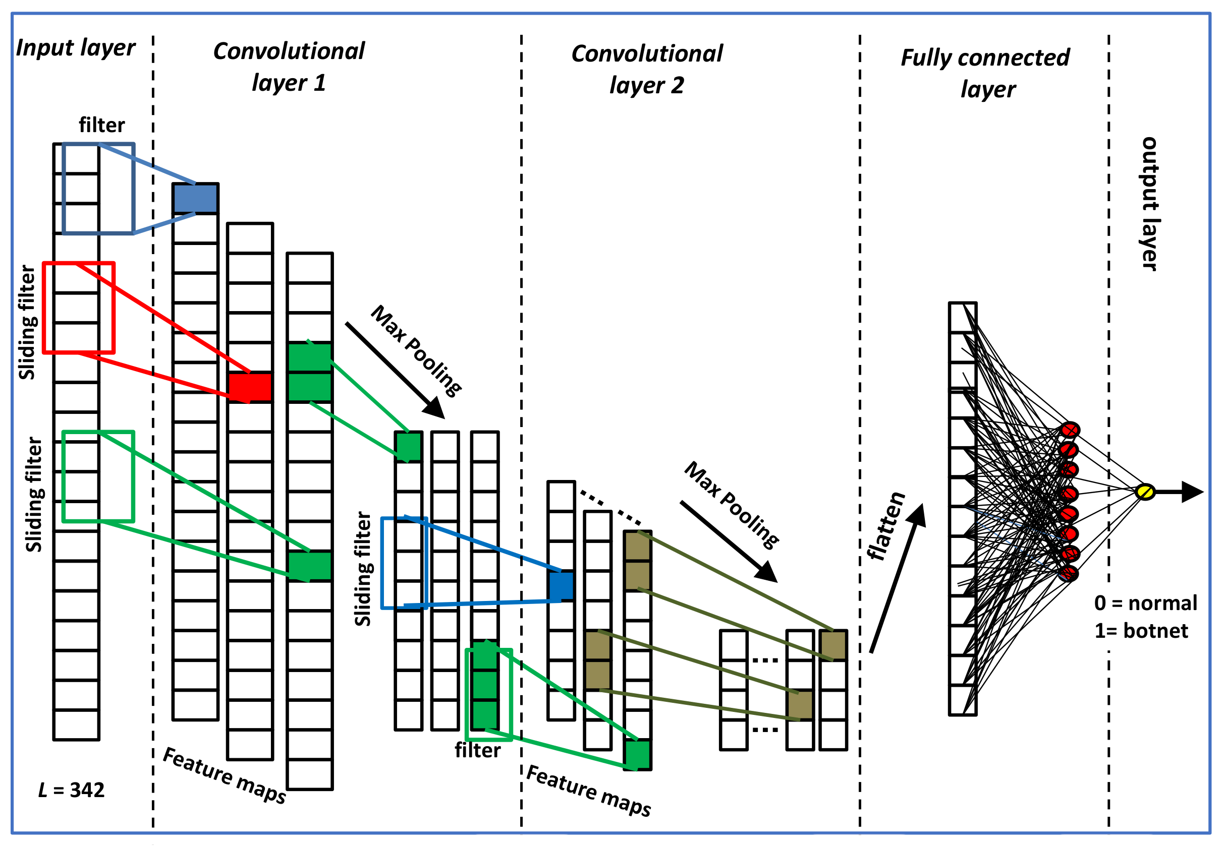
Table 4. In the top half of the table, the configuration had 1 convolutional layer and 1 max pooling layer in the CNN part. These models are named as CNN-1-layer-GRU-X where X stands for the number of hidden units in the GRU layer. The Convolutional layer receives input vector of dimension 342 from the input layer, and it consists of 32 filters each of size = 4. The max pooling layer has its parameter set to 2, which means it would reduce the output of the convolutional layer by half. The outputs from the max pooling layer are concatenated into a flat vector before sending to the GRU layer. As depicted in
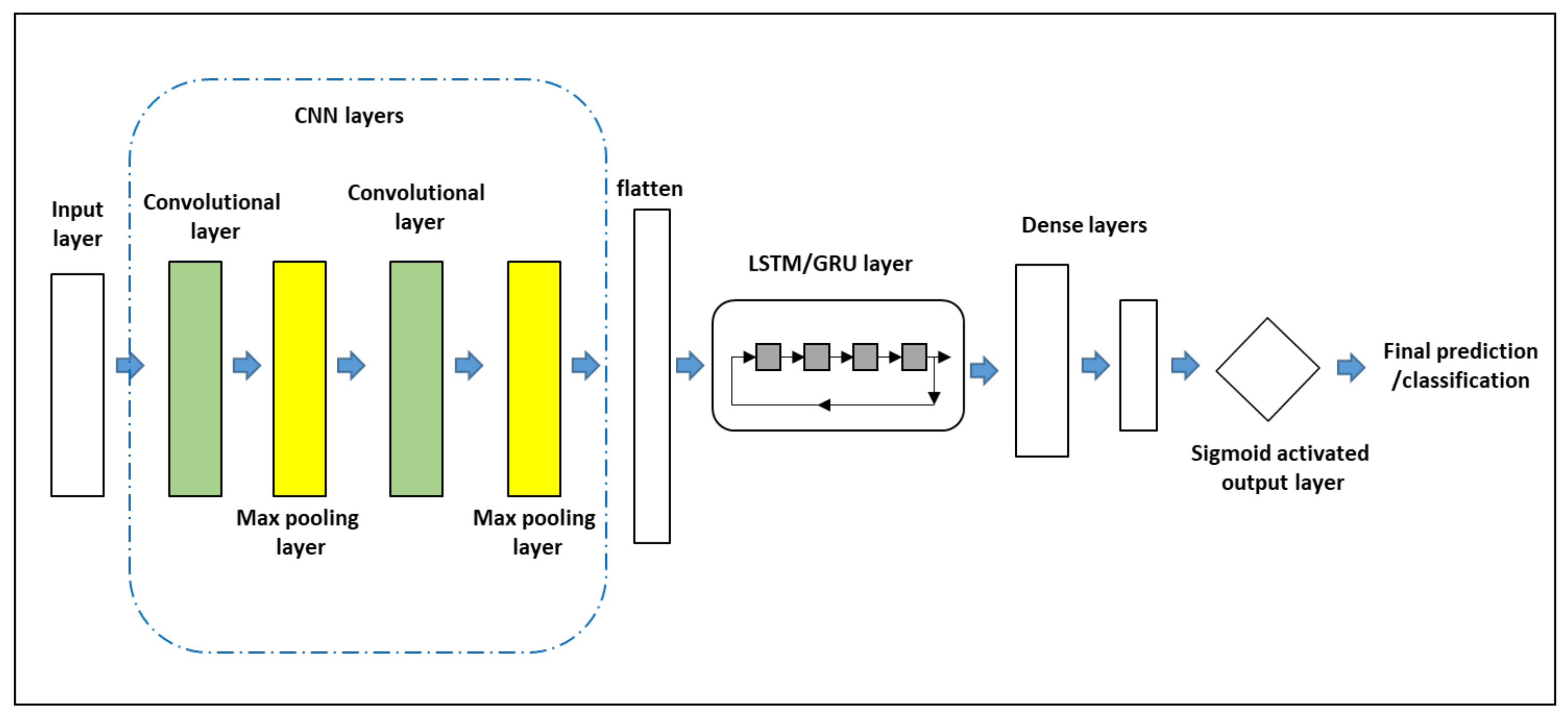
Figure 4, the output from the CNN-GRU layers are forwarded to 2 dense layers. The first dense layer had 128 units, while the second one had 64 units. The 64-unit layer is finally connected to a sigmoid-activated single-unit output layer where the final classification decision into ‘clean’ or ‘botnet’ is made. The model can be summarized in the following sequence:
Input [342] -> Conv [32 filters, Size=4] -> max pooling -> flatten -> GRU[X] -> Dense [128, ReLU] -> Dense[64, ReLU]-> Dense[1, Sigmoid] where X is the number of GRU hidden units taken as 5, 10, 25, and 50, respectively.
The results of the bottom half of
Table 4 are from the same CNN-GRU architecture described above, but with the CNN part having 2 convolutional layers and 2 max pooling layers. The model can be summarized in the following sequence:
Input [342] -> Conv [32 filters, Size=4] -> max pooling -> Conv [32 filters, Size=4] -> max pooling -> flatten -> GRU[X]->Dense [128, ReLU] -> Dense[64, ReLU]->Dense[1, Sigmoid] where X is the number of GRU hidden units taken as 5, 10, 25, and 50, respectively.
Note that a dropout = 0.25 is incorporated between each of the layers in the models to reduce overfitting.
From
Table 4, we can see that the model with the 1-layer CNN had higher overall accuracy of 98.9% when the number of GRU hidden units were set at 10 or at 50. The corresponding F1-score were also the highest at 0.980. The recall of the GRU-50 model was 0.980 compared to that of the GRU-10 model, which was 0.975. This means that the GRU-50 model was better at detecting botnet apps than the GRU-10 model in the top half of
Table 4. Note that the GRU-5 model from the 1-layer CNN batch (top-half) which had 5 hidden units actually did perform well also by obtaining an overall accuracy of 98.8%, with an F1-score of 0.979 and a botnet detection rate (recall) of 97.6%. It had the least numbers of parameters to train, i.e., 90,422.
From the bottom half of
Table 4, the 2-layer CNN models with the best overall accuracy was the one with 50 units in the GRU layer (i.e., CNN-2-GRU-50). It obtained 99.1% accuracy, and the best F1 score of 0.984. The recall (botnet detection rate) was 97.9% while the precision was 98.8%, the highest in all of the CNN-GRU models. From these set of results, we can conclude the following:
The best overall performance for the CNN-GRU models was from the model with 2 convolutional layers and 50 hidden units in the GRU layer.
Very good results can be obtained by CNN-GRU model with only 1 convolutional layer and few hidden units (5) in the GRU layer. The accuracy observed was 98.8%, and the F1 score was 0.979. The lower the number of hidden units, the faster it is to train the model.
6.2. CNN-LSTM Model Results
This section presents the results of the CNN-LSTM models with different configurations in both the CNN layer and the GRU layer. The results are presented in
Table 5. Similar to the results of CNN-GRU in
Table 4, the top half is for the models with 1 convolutional layer and 1 max pooling layer in the CNN part, while the bottom half (of
Table 5) shows the results of the models having 2 convolutional layers and 2 max pooling layers in the CNN part. The models are named with the convention CNN-1-layer-LSTM-X in the top half, or CNN-2-layer-LSTM-X in the bottom half, where X stands for the number of hidden units in the LSTM layer. As depicted in
Figure 4, the output from the CNN-LSTM layers are forwarded to 2 dense layers. The first dense layer had 128 units, while the second one had 64 units. The 64-unit layer is finally connected to a single unit sigmoid activated output layer where the final classification decision into ‘clean’ or ‘botnet’ is made. The model can be summarized in the following sequence:
Input [342] -> Conv [32 filters, Size=4] -> max pooling -> flatten -> LSTM[X] -> Dense [128, ReLU] -> Dense [64, ReLU]-> Dense[1, Sigmoid]
where X is the number of LSTM hidden units taken as 5, 10, 25, and 50, respectively.
For the bottom half of
Table 5, the models can be summarized in the following sequence:
Input [342] -> Conv [32 filters, Size=4] -> max pooling -> Conv [32 filters, Size=4] -> max pooling -> flatten -> LSTM[X]->Dense [128, ReLU] -> Dense [64, ReLU]->Dense [1, Sigmoid]
where X is the number of LSTM hidden units taken as 5, 10, 25, and 50, respectively.
Note that a dropout = 0.25 is incorporated between each of the layers in the models to reduce overfitting.
Table 5 (top half), it can be seen that the all the CNN-LSTM models with only 1 layer in the CNN part had overall accuracy of 99%. The models with 10 and 50 hidden units, respectively, in the LSTM layer obtained identical F1-score of 0.983, compared to the ones with 5 and 25, respectively, which had F1-score of 0.982. The best recall (or botnet detection rate) of 98.3% was recorded with the LSTM-50 model. However, having more than 1.1 million parameters, the LSTM-50 model will be longer to train than the LSTM-10 model which has only 226,617 parameters.
From the bottom half of
Table 5, the 2-layer CNN models with the best overall accuracy was the one with 25 units in the LSTM layer (i.e., CNN-LSTM-25). It obtained 99% accuracy, and the best F1 score of 0.981. The recall (botnet detection rate) was 97.9% while the precision was 98.4%. From the results of
Table 5, we can conclude the following:
The best overall performance for the CNN-LSTM models was from the model with 1 convolutional layer and 25 hidden units in the LSTM layer.
Very good results can be obtained by CNN-LSTM model with only 1 convolutional layer and few hidden units (5) in the LSTM layer. This is evident from the results of the CNN-1-layer-LSTM-5 where the accuracy observed was 99%, and the F1 score was 0.982, precision was 98.7%, and recall (botnet detection rate) was 97.7%.
Comparing
Table 4 and
Table 5, the results of CNN-LSTM were generally better than those of CNN-GRU even though a CNN-GRU model obtained the highest F1-score of 0.984 with an overall accuracy of 99.1%.
6.3. CNN Model Results
In this section we discuss the results of the CNN model which is summarized in
Table 6. The CNN model consists of 2 convolutional layers and 2 max pooling layers. The resulting vectors are ‘flattened’ and fed into a dense layer containing 8 units. The model’s sequence can be summarized as follows:
Input [342] -> Conv [32 filters, Size=4] -> max pooling -> Conv [32 filters, Size=4] -> max pooling-> flatten -> Dense [8, ReLU] -> Dense [1, Sigmoid]
In our preliminary study presented in [
24], this particular configuration of the model has been determined to yield the best performance on the same features extracted from the same app dataset used for the other models presented in this paper. More extensive performance evaluation of the CNN model has been presented in [
24], where the effect of varying the other parameters, such as filter length, number of layers, and max pooling parameter has been investigated.
As shown in
Table 6, the CNN model with 32 filters yielded the best results with 98.9% overall accuracy, precision = 0.983, recall = 0.978, and F1-score = 0.981. When compared to the results in
Table 4 and
Table 5, it can be observed that most of the CNN-LSTM configurations and some of the CNN-GRU configurations achieved higher results than the CNN-only model. This suggests that the LSTM and GRU were able to capture some dependencies amongst the features thus improving the performance of the model.
6.4. DNN Model Results
The results obtained from the Dense Neural Network model is presented in this section. The naming convention used to describe the models is DNN-Y-layer-N as shown in
Table 7, where
Y stands for the number of hidden layers and
N is the number of units in the layer. For example, the sequence of the DNN-2-layer-200 model can be summarized as follows:
Note that a dropout = 0.25 is incorporated between each of the layers in the models to reduce overfitting. Additionally, in all of the DNN models and the previous models in
Section 6.1,
Section 6.2 and
Section 6.3, the optimization algorithm used was ‘Adam’ and ‘Binary cross entropy’ was used for the loss function. Furthermore, all the models were configured to automatically terminate the training after the validation loss is observed to have not changed for a specific number of
K training epochs, where
K was set to 20.
From
Table 7, it can be observed that the DNN models with a single hidden layer did not result in the best outcomes. Likewise, in most cases, using 3 hidden layers as observed with the DNN-3-layer-200 and DNN-3-layer-300 also did not give the best outcomes. The best performance was obtained from the model with 2 hidden layers and 100 units in each layer, where the overall accuracy is 99.1% and F1-score = 0.984. The model with 3 hidden layers and 100 units in each layer also gave identical results. This shows that increasing the number of units in each layer is unlikely to improve the performance any further.
6.5. Best Deep Learning Results vs. Classical Non-Deep Learning Classifiers
In
Table 8, we juxtapose the best results from our investigation of the deep learning classifiers with the results from the classical machine learning techniques. The DNN and the CNN-GRU models achieved the best results as depicted in the table. The highest accuracy achieved by both models were 99.1% which also corresponds to the highest F1-score of 0.984. These results are followed closely by the CNN-LSTM model which achieved 99% overall accuracy and F1-score of 0.983. Next, was the CNN-only model with 98.9% accuracy and F1-score of 0.981. All of these models outperformed the classical machine learning classifiers where the best two were SVM and Random Forest. SVM had 98.7% overall accuracy and F1-score of 0.976, while Random Forest obtained 98.5% accuracy and F1-score of 0.973. These results suggest that with the static based features extracted for detecting Android botnets, the deep learning models will perform beyond the limits of the classical machine learning classifiers.
In the table, the GRU-only model is shown as having the least accuracy results compared to all the other models. This GRU model consisted of 200 hidden units and obtained an overall accuracy of 82.9%. Similarly, with LSTM-only models, overall accuracies below 75% were observed (results not shown in the table). This confirmed our initial expectation that pattern recognition (e.g., with convolutional layers or dense layers) was more important for the type of feature vectors used in the study, rather than context or dependencies. However, the results of
Section 6.1 and
Section 6.2 for the hybrid models suggests that a combination of methods that can capture both characteristics is promising.
6.6. Model Training Times
When training the deep learning models, the number of epochs has a major influence on the overall model training time. In our experiments we utilized a stopping criterion based on minimum validation loss rather than specifying a fixed number of training epochs. For this reason, the number of training epochs varied between the different configurations of a given model. Hence, the longest CNN-GRU model to train was the CNN-2-layer-GRU-25 which took 145 s, and the testing time was 0.482 s. Whereas the shortest CNN-GRU model to train was the CNN-1-layer-GRU-10 model which took 84.4 s with a testing time of 0.399 s. The longest CNN-LSTM model to train was the CNN-2-layer-LSTM-5 which took 141 s with a testing time of 0.468 s. The shortest CNN-LSTM model to train was the CNN-1-layer-LSTM-25 model which took 83.6 s with a testing time of 0.419 s. Compared to the other models, the DNN was the fastest to train with training times ranging from 10 to 26 s and an average testing time of 0.15 s.
6.7. Comparison with Previous Works
The results obtained in our study improves the performance beyond the reported results in previous papers that also used the ISCX botnet dataset in their work. This can be observed in
Table 9. The second column shows the numbers of the botnet and benign samples used in each of the referenced paper. Note that in some papers, some of the metrics were not reported. Even though the complete datasets and techniques used were different in each of the previous works,
Table 9 shows that the models developed in this paper achieved state-of-the-art results with the ISCX botnet dataset compared to the others.


