Article

Deep Learning-Based Content Caching in the Fog Access Points

1
IoT and Big-Data Research Center, Department of Electronics Engineering, Incheon National University, Yeonsu-gu, Incheon 22012, Korea
2
Department of Computer Science and Engineering, Incheon National University, Yeonsu-gu, Incheon 22012, Korea
*
Author to whom correspondence should be addressed.
Electronics 2021, 10(4), 512; https://doi.org/10.3390/electronics10040512
Submission received: 29 January 2021 / Revised: 15 February 2021 / Accepted: 18 February 2021 / Published: 22 February 2021
(This article belongs to the Special Issue Edge Computing for Internet of Things)

Abstract

:
Proactive caching of the most popular contents in the cache memory of fog-access points (F-APs) is regarded as a promising solution for the 5G and beyond cellular communication to address latency-related issues caused by the unprecedented demand of multimedia data traffic. However, it is still challenging to correctly predict the user’s content and store it in the cache memory of the F-APs efficiently as the user preference is dynamic. In this article, to solve this issue to some extent, the deep learning-based content caching (DLCC) method is proposed due to recent advances in deep learning. In DLCC, a 2D CNN-based method is exploited to formulate the caching model. The simulation results in terms of deep learning (DL) accuracy, mean square error (MSE), the cache hit ratio, and the overall system delay is displayed to show that the proposed method outperforms the performance of known DL-based caching strategies, as well as transfer learning-based cooperative caching (LECC) strategy, randomized replacement (RR), and the Zipf’s probability distribution.

1. Introduction

With the blooming of IoT devices, it is expected that the demand for mobile data traffic will grow at an unprecedented rate. To solve this issue to some extent, cisco coined fog computing-based network architecture to address latency-related problems [1]. Fog computing is a decentralized version of cloud computing with limited computational and signal processing capability, which brings the benefit of cloud computing nearer to the user side [2]. The remote radio heads with caching and signal processing capabilities in the fog computing architecture are referred to as fog access points (F-APs) [3,4]. F-APs have limited computational capability as compared to the cloud. So, F-APs should store popular cache contents proactively to maintain desirable fronthaul load to provide a better quality of service [5,6,7].
There has been extensive research related to caching in F-APs. Some of the related works are worth mentioning. In [8], the learning-based optimal solution is provided to place a cache memory content in a small cell base station based on the historical data. In [9], based on the user’s mobility, a device-to-device optimal contents placement strategy is introduced. Likewise, in [10], the caching problem in multiple fog-nodes is studied to optimize delay in the large-scale cellular network. Similarly, in [11], the authors formulated; delay minimization and content placement-based joint optimization problems.
In the aforementioned literature [8,9,10,11], the research predicted the popularity of the contents based on Zipf’s probability distribution method. However, this method cannot accurately predict the user content as user behavior is dynamic.
AI is likely to bring the fourth industrial revolution due to recent advances in its field [12]. There has been increased interest in deep learning (DL) models due to their remarkable impact in a wide variety of fields such as natural language processing, computer vision, and so on [13,14].
Recently, there has been more focused research on the DL-based approach to predict the future popular contents to solve the prevalent cache content placement issue [15]. In this paper, motivated by the DL-based approach, we propose a DL-based content caching (DLCC) to proactively store cache contents in the fog computing environment.

1.1. Related Works

The concept of fog radio access network (F-RAN) architecture had been introduced to bring cloud contents nearer to the end-users side, such that the fronthaul burden prevalent in the cloud radio access networks can be lessened. The cloud contents can be offloaded nearer to the end-user side by deploying the proper content caching technique in the F-APs.
In recent years, there has been enormous investigation to address content caching problems for wireless networks. The work of [16] discussed a joint routing and caching problem to maximize the portion of contents served locally by the small base stations in the cellular networks. In [17], femtocell caching followed by D2D-based content sharing idea is put forward to improve cellular throughput. The work of [18] focused on the latency-centric analysis of the degree of freedom of an F-RAN system for optimal caching and edge transmission policies. The works in [16,17,18] did not consider taking popular contents into account to address caching problem.
Since the F-APs have limited storage as well as signal processing capabilities, the highly preferred user contents should be placed in the cache memory of the fog nodes. The traditional approach of allocating cache contents in the wireless networks includes; least recently used, least frequently used, first-in-first-out, random replacement (RR), and time-to-live [19]. These methods have become impractical to use in the live network as user requirement changes over time. To mitigate the traditional approach of solving caching problems, some authors recommended placing the cache contents by analyzing the user’s social information. In [20], social-aware edge caching techniques have been studied to minimize bandwidth consumption. In [21], social information and edge computing environment have been fully exploited to alleviate the end-to-end latency. However, social ties alone cannot be a sole deterministic factor to determine the dynamic nature of user preference.
Lately, there has been a marked increment in the utilization of big-data analytics, ML, and deep learning (DL) in academia, as well as in industry. They have been used to solve problems related to diverse domains such as autonomous driving, medical diagnosis, road traffic prediction, radio-resource management, caching, and so on, due to their high prediction accuracy [22,23,24]. Due to promising solutions provided by the artificial intelligence (AI) technology in various domains, a trend to exploit ML-based and DL-based models to the pre-determined future requirement of the user content has been set-up.
For instance, the works which have used an ML-based approach to determine the cache contents proactively are listed in [25,26]. In [25], a collaborative filtering (CF)-based technique is introduced to estimate the file popularity matrix in a small cellular network. However, the CF algorithm provides the sub-optimal solution when the training data are sparse. To solve the caching problem without undergoing any data sparseness problem, the authors in [26] proposed a transfer learning (TL)-based approach. However, in this approach, if similar content is migrated improperly, the prediction accuracy becomes worse.
Likewise, some of the papers, which have used DL-based models to forecast popular contents for caching are listed in [15,27,28,29]. In [15], an auto-encoder-based model is used to forecast the popularity of the contents. Likewise, in [27], a bidirectional recurrent neural network is used to determine content request distribution. In [28], a convolutional neural network-based caching strategy is presented. Moreover, in [29], the authors used different DL-based models such as a recurrent neural network, convolutional neural network (CNN), and convolutional recurrent neural network (CRNN) to determine the best cache contents and increase the cache hit ratio. However, in the above works, the DL-based model could not achieve validation accuracy greater than 77%. Therefore, accurately predicting F-APs cache contents with DL-models has become a challenging task.

1.2. Contribution and Organization

In this paper, to minimize the delay while accessing users’ content, a DLCC strategy is introduced to store the most popular users’ contents in the F-APs. In DLCC policy, we introduced a supervised learning-based 2D CNN model to train using 1D real-world datasets. We identified key features and key labels of the datasets by different data pre-processing techniques such as data cleaning, one-hot encoding, principal component analysis (PCA), k-means clustering, correlation analysis, and so on. The goal of our DLCC algorithm is to predict the popularity of contents in terms of different categorical classes. Then, based on the prediction result, the data of the most popular class will be stored in the cache memory of the nearby F-APs. We quantified the performance of the proposed caching policy on F-APs by showing DL accuracy, cache-hit ratio, and overall system delay.
The methodology of this article is shown in Figure 1 and summarized as follows:
  • An optimization problem to minimize content access delay in the future time is introduced.
  • DLCC strategy is proposed.
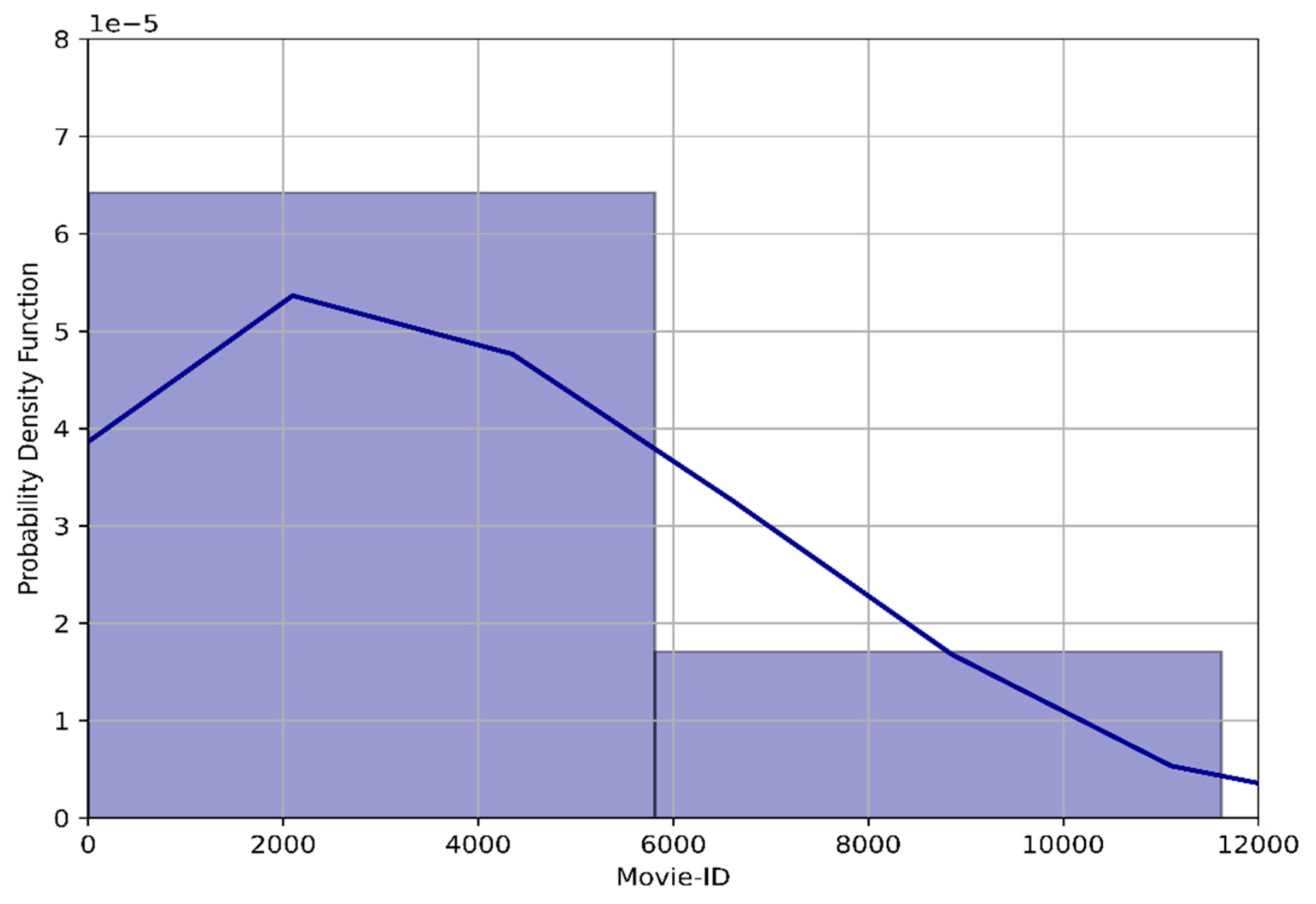
  • Open access real-life large dataset, such as MovieLens dataset [30] is analyzed and formatted using different data pre-processing techniques for the proper use for supervised DL-based approach.
  • 2D CNN model is trained using 1D dataset to obtain the most popular future data.
  • The most popular data are then stored in the cache memory of the F-APs.
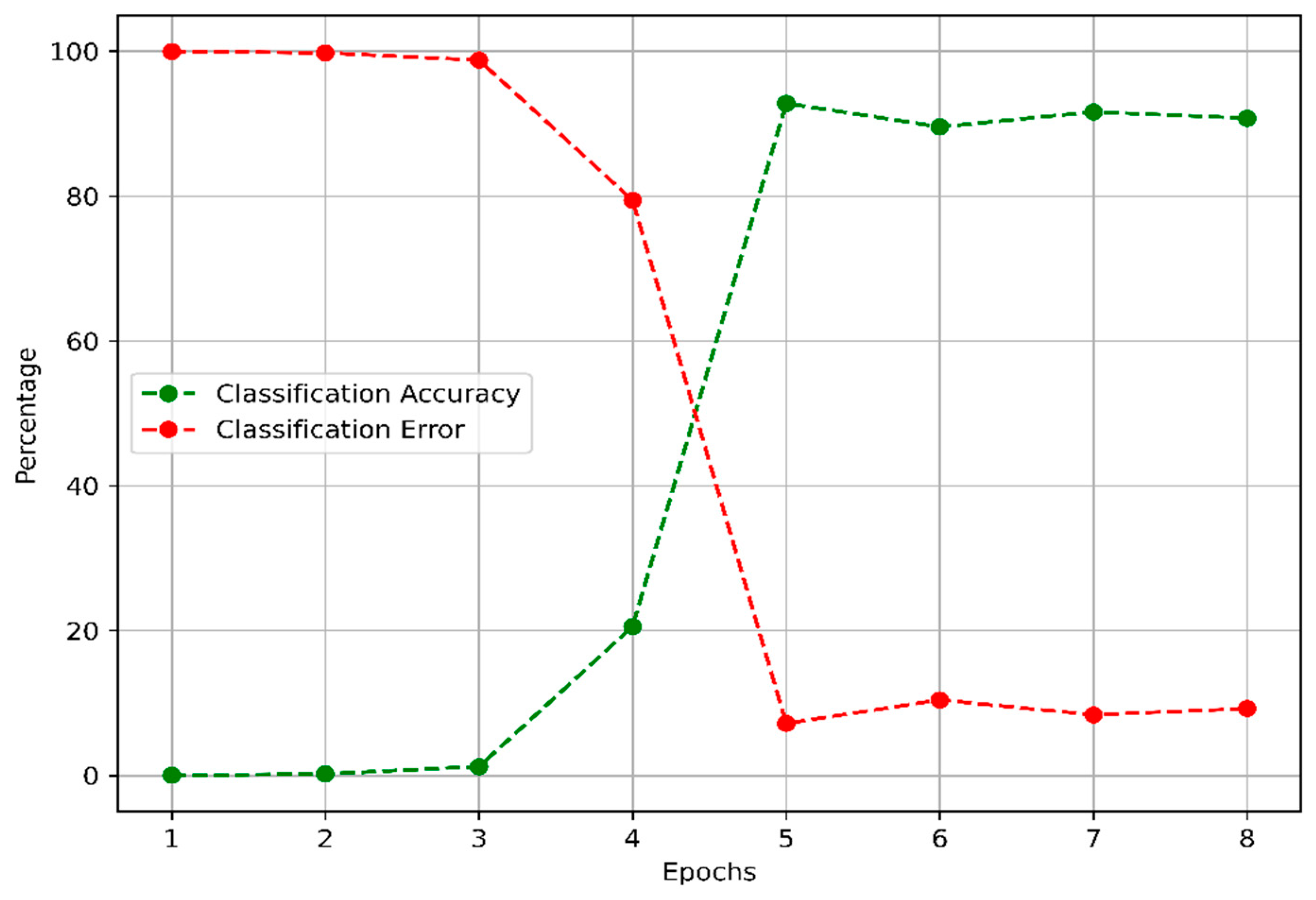
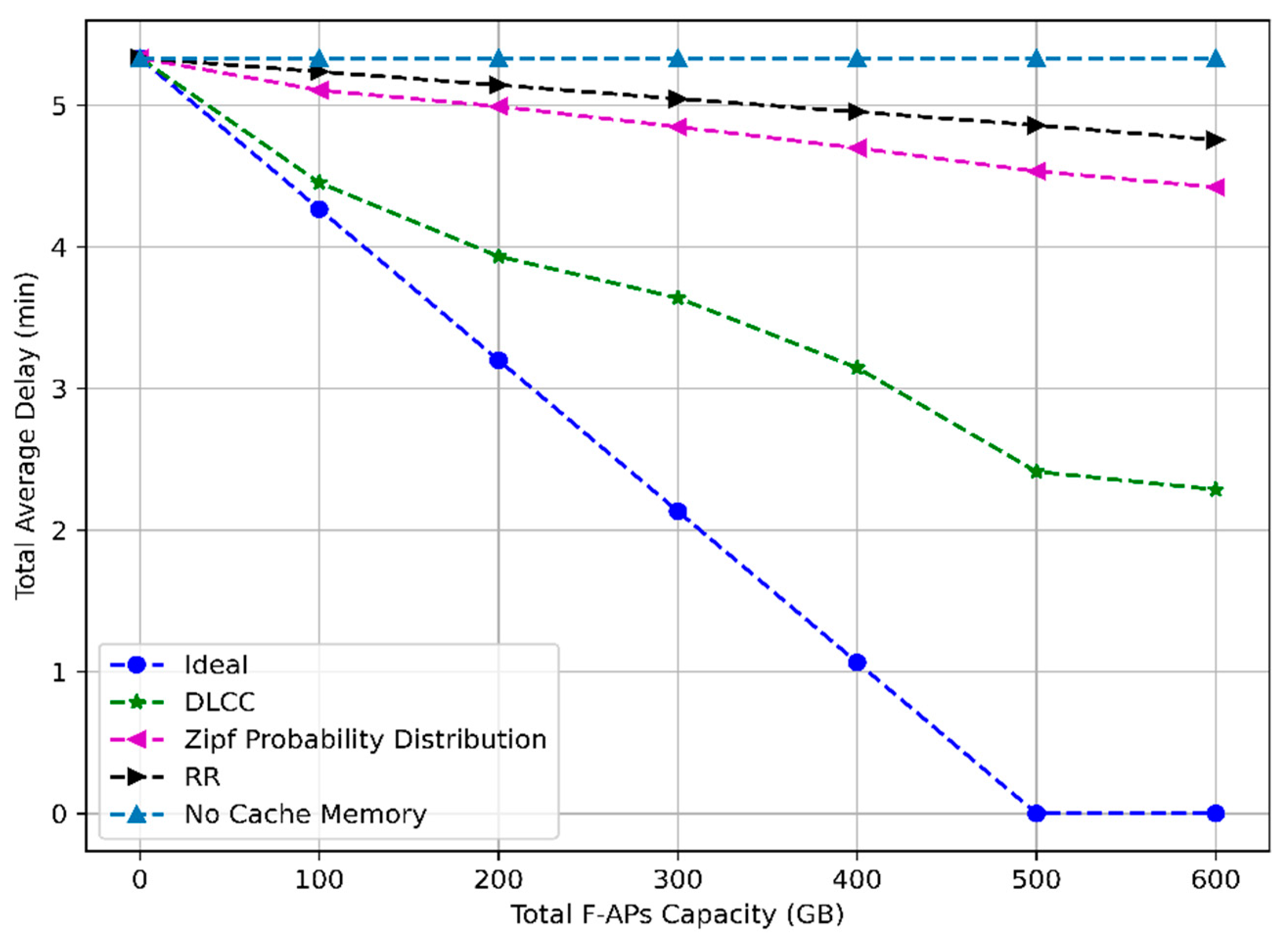
  • The performance is shown in terms of mean square error (MSE), DL-accuracy, cache hit ratio, and overall system delay.
The remainder of this paper is organized as follows; In Section 2, the system model is described. In Section 3, the DLCC policy is presented. Then, in Section 4, the performance of the proposed scheme is evaluated. Finally, in Section 5, conclusions are drawn.

2. System Model

In this section, a caching scenario for N × M fog radio access network (F-RAN) system having N user equipment (UEs), M F-APs, and one centralized base-band unit (BBU) cloud is modeled, as shown in Figure 2. In the system model diagram, we have U = { 1 , 2 , 3 , , N } as the set of N users requesting data from = { 1 , 2 , 3 , M } as the set of M F-APs. In the diagram, the solid line connecting the BBU cloud to the access points represents the common public radio interface (CPRI) cable; whereas, the dashed-lines connecting the end-users to the access points denote the air-interface link.
As per the system model diagram, the DL-based training is done on the centralized cloud (CC) considering the proactive as well as the reactive caching case. The testing results provided by the DL-based model on the CC are used to send the most popular contents to the F-APs. Since the computational capabilities of the F-APs are way lesser than that of the cloud, only the top most popular contents are stored in it. The contents stored in the F-APs are based on location-based user preference. Based on the proactive and reactive caching scenario in an F-RAN system, the delay system is formulated and is shown in part 2.1.

2.1. Delay Formulation

In this part, we are interested in formulating overall system delay for the N × M F-RAN system, for some time instance t + 1 . We assumed that the air-interface link capacity connecting the UE i ( i   U ) to F-AP j ( j   ) as C i , j A i , and the fronthaul link capacity connecting F-AP j to the CC as C j , 1 F h . For simplicity, we considered that the cache memory of all the F-APs has the same capacity to store the files, i.e., (GB). We also assumed that the size of each file p cached at the fog nodes is the same. Let S i , j t + 1 denote the file size requested by the UE i with F-AP j , at any time instance t + 1 . In our problem formulation, for direct transmission, we considered only the delay for transferring the data from the cloud to the F-APs. On the other hand, for cached transmission, the delay for offloading the cached contents from the F-APs to the UEs is neglected. Considering the above scenario, the overall delay for the N × M F-RAN system for any time instance t + 1 can be devised as:
P ( 1 )   δ s y s t + 1 = min   [ i = 1 N j = 1 M ( 1 x i , j t + 1 ) S i , j t + 1 C j , 1 F h ]
s . t .   S i , j t + 1 x i , j t + 1   i , j
where δ s y s t + 1 is the overall delay of the F-RAN system at time t + 1 , and x i , j t + 1 is the decision control variable to show whether the file requested by the UE i with F-AP j at any time t + 1 is available in the cache memory of the latched F-AP, or not. The value of x i , j t + 1 can either be 1 or 0, not otherwise. This can be represented as:
x i , j t + 1 = { 1 ,    if   the   content   requested   by   UE   i   is   available   in   F AP   j 0 ,    otherwise
The constraint in the problem statement (P1) indicates that the size of the file cached in the cache memory of F-AP should be lesser than or equal to the overall memory size of that particular F-AP.

3. DL-based Caching Policy

In this section, DLCC is presented, so that the overall delay of the F-RAN system formulated in (P1) can be minimized in the best possible way. The general overview of the proposed caching policy is shown in Figure 3.
Figure 3 contains a series of the task required for predicting the best cache contents for the F-APs. The initial step includes the extraction of the most popular 1D real-life datasets from the cloud. After the initial step, the downloaded data are pre-processed using various techniques to make it a suitable 2D dataset for the preferred supervised DL-based model. Then, the suitable 2D dataset is trained using the 2D CNN model. After that, the trained model is used to predict the contents on the basis of different categorical classes for time t + 1 . Due to the memory constraint of the F-APs, only the contents of the top-most class are selected randomly to be stored in the F-APs for future user requirements. The steps mentioned above are coherently described in the subsections given below.

3.1. Dataset

MovieLens dataset is used for training the DL-based model, as it is a large dataset available in the open-source platform. Moreover, live streaming of the movies utilizes most of the fronthaul capacity. So, to lessen fronthaul load to some extent, proactive storing of the most popular movies in the cache memory of the F-APs is considered the most viable approach.
We downloaded the MovieLens dataset from [30]. It contains around 25 Million ratings and around 1 Million tag applications for 62,423 movies. Moreover, the dataset contains movies from 1 January 1995 to 21 November 2019, rated by 162,541 users. This dataset was generated on 21 November 2019. In this dataset, random users represented by a unique id had rated at least 20 movies. The data contained in this dataset represent genome-scores.csv, genome-tags.csv, links.csv, ratings.csv, and tags.csv.

3.2. Data Pre-Processing

It requires a large computational effort and also not relevant to train the whole MovieLens dataset, so the portion of the dataset is only taken for training and validation purposes. We used data from 1 January 2015 to 21 November 2019 from the dataset. The selected portion of the dataset contains only around 7.5 million ratings for 58,133 movies.
The initial dataset contains the categorical variable such as User-ID, Movie-ID, Rating, Date, Year, Month, Day, and Genres. Based on the dataset key features such as Year, Month, and Day, the daily requested movies are counted and are portrayed in the form of a yearly-based box plot, as shown in Figure 4.
As per Figure 4, we can see that on average, around 800 movies are requested daily. Likewise, the maximum movie request on a particular day is around 38,000, whereas the minimum movie request is 1.
If we go with the average daily request for the movie, it is still beyond the computational capacity of the F-AP to store 800 movies in its cache memory. To solve this, the dataset is further analyzed on the basis of the Movie-ID and daily movie request count, and it is depicted in Figure 5.
Figure 5 shows the probability density function (PDF) of the Movie-ID based on the movies requested. As per the figure, we can observe that the PDF is comparatively higher for the movie id number within 0–12,000. The PDF is smaller for the movies having id numbers greater than 12,000. Thus, for our analysis, movies with id numbers 0–12,000 are taken into account. The PDF of the selected movies is shown in Figure 6.
After selection of Movie-ID from 0–12,000, the number of rows in the dataset is reduced to around 3.5 Million from 7.5 Million. This selected portion of the dataset accounts to be around 14% of the total dataset (25 Million). Then, the per-day count of the movie as per the unique Movie-ID is calculated to further reduce the number of rows to around 1.6 Million. After that, the dataset is re-arranged as per Movie-ID with its corresponding attributes such as year, month, day, genre, and movie counter.
In the dataset, the genre feature contains the string values. Since the genre feature in the dataset contains the different categorical string values, it is further processed by the One-Hot Encoding method to convert it into numerical form, as the DL-model employs on the numerical data. One-Hot encoding is one of the natural language processing techniques to convert categorical string variables into a numerical form such that machine learning algorithms can perform better prediction [31].
When the One-Hot Encoding technique is applied to a genre column containing multiple categorical string variables, the single genre column is transformed into 19 columns, as it contained 19 different categories. The increment in the column numbers adds up computational complexity to train the model. Therefore, to reduce the computational complexity, principal component analysis (PCA) of the categorical variable of the genre data is performed. PCA is a robust approach for reducing the dimension of datasets; by preserving most of the useful information. It does so by creating new uncorrelated variables that successively maximize variance [32].
The PCA analysis on 19 categorical columns is done to reduce 19 categorical columns to 3 categorical columns. The newly formed categorical columns are named PCA-1, PCA-2, and PCA-3, respectively. Figure 7 shows the individual and cumulative weightage of variance provided by the formed three principal components. In the figure, the first, the second, and the third principal components are indicated by the x-axis values 0, 1, and 2, respectively. The three principal components contain the Eigen-values of the PCA-1, PCA-2, and PCA-3, respectively. We reduced the 18-columned matrices to 3-columned matrices because the cumulative sum of the variance of three principal components accounted for 45.70% of the total variance. As per the figure, the Eigen-values of PCA-1, PCA-2, and PCA-3 contributed 19.66%, 15.59%, and 10.45% of the total variance, respectively. The portion of the variance contributed by PCA-1 is greater, so it is referred to as principal component 1. Since the portion of the variance contributed by the Eigen-values of succeeding columns is lesser than the preceding, they are indicated as principal component 2 and principal component 3, correspondingly.
After the column reduction technique is applied to the dataset, the 1D dataset is converted to a 2D dataset for the selected 9019 Movie-ID’s. There are around 1787 days from the starting of 2015 to 21 November 2019. When 9019 Movie-ID’s is multiplied to 1787, the resulting 2D dataset will have 16,107,934 rows. This is a 1000% increment in the size of the dataset from the reduced version of the 1D dataset.
The resulting 2D dataset is clustered based on per day’s movie request count to add label to the dataset. The dataset is categorized into four categories, i.e., Class 0, Class 1, Class 2, and Class 3, by using the k-means clustering technique, as shown in Figure 8.
In Figure 8, Class 0 is represented by the purple color. This class includes Movie-ID having the almost higher count on a particular day. Likewise, Class 1, Class 2, and Class 3 are represented by the blue, green, and yellow colors, having a range of values such as 12–362, 4–11, and 1–3, respectively. In our 2D dataset, Class 0, Class 1, Class 2, and Class 3 contains 22,604, 212,759, 1,406,486, and 14,736,655 rows, respectively. The Class 0 movies are referred to as highly preferred movies, whereas Class 3 movies are regarded as the least requested ones. These categorized values are placed under the column name Class of the dataset.
The resulting dataset contains Year, Month, Day, Movie-ID, PCA-1, PCA-2, and PCA-3 as the key features, and the Class as a key label. The correlation matrix in Figure 9 is shown to depict the usefulness of our dataset for the 2D CNN model.

3.3. DLCC Model

In this section, at first, we explain the problem statement and then discuss the architecture for predicting the future popularity of movies listed in the MovieLens dataset by using the time-series sequence of historical data.

3.3.1. Problem Statement

The main objective of the DLCC model is to realize the future likelihood of the data contents being accessed by the connected UEs. In this study, the DLCC model is trained based on the MovieLens dataset d , containing movie lists up to time t . Let Χ = { X 1 ,   X 2 ,   X 3 ,   , X t } be the chronological order of time-variant historical movies list. Its corresponding output label, which is particularly the classification of movies list based on popularity, can be represented as Y = { Y 1 ,   Y 2 , Y 3 , , Y t } . The i t h time input of Χ . can be denoted as:
X i = [ x 11 i x 12 i x 1 f i x 21 i x 22 i x 2 f i x n 1 i x n 2 i x n f i ] n × f
ere X i contains collection of n movie samples, each having f features. Similarly, its corresponding i t h time output label can be represented as:
Y i = [ y 1 i y 2 i y n i ] n × 1
where Y i contains the category of each movie sample based on popularity. The primary objective of this study is to develop the prediction model , which uses input features X i to predict the popular class Y i , which can be defined as:
Y i = ( X i ,   θ )
where θ is the model parameter of DLCC model.

3.3.2. Model Implementation

In this part, we use 2D CNN for feature extraction from the input 2D MovieLens dataset. Moreover, we use a regression-based approach to solve the classification problem. The main goal of the DLCC model is to categorize MovieLens dataset on the basis of popularity. The DLCC model used in this paper is shown in Figure 10.
In Figure 10, the architecture of the DLCC model is formed by stacking three convolutional layers, two max-poling layers, one flatten layer, and one dense layer. Mathematically, the f t h feature map of l t h   convolutional layer y f l can be obtained by first convoluting 2D input or previous layer output with the convolutional filter and then applying bit-wise non-linear activation, which is shown in Equation (7).
y f l = σ ( k = 1 f l 1 y k l 1 W k f l + b f l ) ,   f [ 1 , f l ]
where y k l 1 is the k t h feature map of ( l 1 ) t h layer, W k f l is the kernel weight at position k connected to the f t h feature map of l t h layer, b f l is the bias of f t h filter of l t h layer, f l is the number of the filter in l t h layer and σ ( . ) represent element-wise non-linear activation function. Equation (8) shows the output of l t h convolutional layer and pooling layer.
y f l = p o o l ( σ ( k = 1 f l 1 y k l 1 W k f l + b f l ) ) ,   f [ 1 , f l ]
In the DLCC model, the feature learned from the 2D CNN model is concatenated into a dense vector by flattening operation. The dense layer contains the high feature extraction from the input. Let L be the previous layer before flattening layer, having f L number of feature maps, then the output of L + 1 layer, y L + 1 is given as:
y L + 1 = o f l a t t e n L = f l a t t e n ( [ y 1 L ,   y 2 L ,   ,   y f L L ] )
where y 1 L , y 2 L , ,   y f L L are the feature maps of L t h layers, and o f l a t t e n L is the flatten vector of L layer. Finally, the flattened layers are transformed to model output through a fully connected layer, having W d and b d weight and bias of fully connected dense layer. The model output can be written as:
y ^ = W d o f l a t t e n L + b d = W d ( f l a t t e n ( p o o l ( σ ( k = 1 f l 1 y k l 1 W k f l + b f l ) ) ) ) + b d
In our model MSE loss function ( θ ) is used to optimize the target. Minimizing MSE is taken as the training goal of our model. Mathematically, MSE can be written as:
( θ ) = y t y ^ t 2 2
In Figure 10, at first 2D input of size 9019 × 7 (rows number × column numbers) is employed to the first convolutional 2D layer of the portrayed DLCC model. In the first convolutional layer, the input is scaled up by using 32 filters of size 2 × 2 with a stride of 1 × 1. The convoluted output of the first layer is then fed to the downsampling layer. In the downsampling layer, the max-pooling technique with a pool size of 2 × 2 is used along with the batch normalization (BN) and dropout techniques. In our DLCC model, BN is used to stabilize the learning process and reduce the number of epochs required to train the neural networks [33], whereas dropout is used to prevent the trained model from overfitting [34]. The convoluted downsampled data of size 4509 × 3 × 32 are employed in the second convolutional layer to reduce the filter number from 32 to 16 by using the same filter and stride size used in the first convolutional layer. After that, the convoluted outputs of the second convolutional layer are again employed in the downsampling layer to reduce the size of inputs to 2254 × 1 × 16. Again, the downsampled data of the second downsampling layer are fed to the third convolutional layer to reduce the filter size from 16 to 8. Since the necessary features were extracted after the implementation of the third convolutional layer, the features of size 2254 × 1 × 8 are flattened to employ it to the fully-connected neural network (FCNN) for the regression process. In each convolutional layer, a rectified linear unit (ReLU) activation function is used to increase the non-linearity in our input data, as well as to solve a vanishing gradient problem. In the regression process, the input of size 18,032 is fed to the FCNN layer to get the output of size 9019. The detailed structure of our DLCC model is shown in Table 1.
In the output of FCNN, the ReLU activation function is used to get output greater than one. After the implementation of the ReLU activation function, the predicted outputs are rounded-off to make hard-decision. The obtained hard-decision is the classification of the MovieLens dataset based on popularity. We trained 1461 data of size 9019 × 7 to predict output for time t n + 1 .
Algorithm 1: Training process for DLCC model.
Electronics 10 00512 i001
Since our problem is a multi-variant regression problem, the mean square error method is used in the training process [35]. Moreover, the Adam optimizer is used to update the weight and learning rate values as it is straightforward to implement, computationally efficient, and has low memory requirements [36]. It is very difficult to tune the hyper-parameters required to train the DL model. The detailed procedure to select hyper-parameters such as batch size (b) and learning rate ( α ) to train the proposed model ( m ) is shown in Algorithm 1.
In Algorithm 1, the CNN model m is trained for the random values of batch size m b and learning rate m α . For each value of m b , 1000 random learning rates having a value in between (0, 1) is realized to train on dataset d . The value of m b is selected by increasing the power of base integer two from 0–9. Using every value of m b and m α , the model is trained on dataset d to obtain training error ( m t e r r o r ) and validation error ( m v e r r o r ), which is stored in the v a l array. After the completion of the loop, the k t h index on the v a l array providing the minimum value of m t e r r o r and m v e r r o r is selected to extract the hyper-parameters value stored in that particular index. Finally, the obtained hyper-parameter values are selected to train the model m to get trained model m k .
Choosing the depth of convolutional neural network plays a crucial role in determining the performance of the model as each addition of convolutional layer in the model leads to the increment of the feature map, so the learning. However, beyond a certain limit, each addition of a convolutional layer in the model tends to overfit the data. So, based on DLCC model accuracy, we experimented using different depths of the model to find a better one. Table 2 justifies why we only chose three convolutional layers in our model.
As per Table 2, we can see that the DLCC model having the single convolutional layer could not provide any output because of the large number of trainable parameters, i.e., 39B. The MSE is minimum for the DLCC model having three convolutional layers in its architecture with a filter configuration of 64_32_8, while the computational time is lesser for the DLCC model having four convolutional layers. Since we require to select the model which provides minimum MSE in a reasonable time, we selected the DLCC_3_1 model to solve the caching issue. The validation MSE provided by the DLCC_3_1 model at the cost of 13.35 min is 0.0452. The number of the input parameters and hyper-parameters was the same for generating results for all four configurations.
Furthermore, the number of filters in the convolution neural networks also plays an important role in determining the performance of the model. So, to find out the best filter configuration for our DLCC_3_1 model, we tried three different configurations, as shown in Table 3.
Table 3 shows that the DLCC_3_1 model having filter configuration 32_16_8 provides a better validation loss as compared to the other two different types of filter configuration. So, we selected the filter configuration of 32_16_8 for our DLCC_3_1 model.

3.4. Cache Decision

In this part, caching decision process is described to allocate the best cache contents to F-APs. The initial step includes the training of the DLCC model on the cloud, based on Algorithm 1. Then the trained model is used to predict cache contents for time t + 1 . After that, the list of contents categorized based on popular classes is transferred to the F-APs for the selection process. On the priority order, the contents of Class 0 is stored in the available cache memory of the F-APs. If the is still some memory available, the contents of Class 1 followed by Class 2 are recommended to be stored in the available cache memory. The contents of Class 3 are not stored even if there is any memory space available in the F-APs as contents of Class 3 are the least preferred ones. The detailed procedure is summarized in Algorithm 2.
Algorithm 2: Cache content decision process.
Electronics 10 00512 i002

4. Performance Analysis

In this section, the performance of the proposed CNN-based model is shown in terms of model key performance indicators (KPI): such as MSE and prediction accuracy. Likewise, the performance cache content decision is quantified in terms of cache hit ratio and system delay.
To train the DLCC model, we used the Keras library on top of the TensorFlow framework in Python 3.7 as a programming platform. The training process for our datasets is performed by using a computation server (MiruWare, Seoul, Korea). The specification of the computational server includes; one Intel Core i7 CPU, four Intel Xeon E7-1680 processors, and 128 GB random access memory. The results are obtained by using a computer with 16 GB random access memory and an Intel Core i7-8700 processor.

4.1. Model KPI

In this part, the DLCC model KPI in terms of MSE (regression), and prediction accuracy (classification) is presented. The proposed 2D CNN-based model is trained on each day data of the MovieLens dataset from January 2015–December 2018. Likewise, the validation of the trained model is done on the data of January 2019–October 2019. Finally, the trained model is tested on the data of November 2019. The simulation parameter used while training the model is summarized in Table 4.
Before the application of hard-decision on the obtained results, the MSE obtained while testing the trained model on the November 2019 data of MovieLens dataset is shown in Table 5. The obtained result is compared with the results shown in [29].
The hard-decision rule is implemented for classifying the prediction results of the CNN-based regression model, which is shown in Table 6.
After the implementation of mapping table shown in Table 6, the average value of prediction accuracy and prediction error of November 2018 is shown in Figure 11 for the different values of training epochs.
As per Figure 11, it can be seen that there is an exponential rise in the prediction accuracy of the model and exponential decay in the prediction error of the model till the five training epoch. Beyond the five training epoch, the learning potential of the model enters the saturation phase. The prediction accuracy of the model is 92.81% for the five training epochs, but it is around 1% for the training epoch less than four. Moreover, the error curve shown in Figure 11 is plotted based on the formula; C l a s s i f i c a t i o n   E r r o r   ( % )   =   100   ( % )     C l a s s i f i c a t i o n   A c c u r a c y   ( % ) .
To lime-light the prediction accuracy of each class, a multi-class confusion matrix is drawn for the prediction date: 1 November 2019 to 21 November 2019. The confusion matrix value of the whole testing period is averaged and is shown in Table 7. The accuracy of the confusion matrix shown in Table 4 can be calculated using the following formula [37]:
A c c u r a c y = T P + T N T P + T N + F P + F N
where “TP”, “TN”, “FP”, and “FN” corresponds to “true positive”, “true negative”, “false positive”, and “false negative”, respectively. Using the above equation, the value of the accuracy for the confusion matrix shown in Table 7 is calculated to be 92.81%. This accuracy is around 21–54% greater than the prediction accuracy reported in the papers [15,27,28,29] while solving a similar problem.

4.2. System KPI

In this section, the cache hit ratio and overall system delay are shown to portray the usefulness of the DLCC policy in the F-RAN system. The movies of the categories “0”, “1” and “2” are proactively stored in the F-APs, whereas the movies under category “3” are not stored as they are the least preferred ones.
Mathematically, the cache hit ratio for any time instance can be calculated as:
C a c h e   h i t   r a t i o   ( t ) = T o t a l   c a c h e   h i t s   ( t ) T o t a l   c a c h e   h i t s   ( t )   +   T o t a l   c a c h e   m i s s e s   ( t )
The system parameters used to calculate the cache hit ratio and the system delay are summarized in Table 8.
As shown in Table 8, an F-RAN system consisting of 50 F-APs and 400 UEs is designed to request movie files from the pool of files. It is assumed that each user can request only one movie file from F-APs at time t + 1 . Likewise, the size of each movie file listed in the MovieLens dataset is considered to be 1 GB, making a total of 9019 GB. Since there are 400 UEs in our system, 400 movie requests at time t + 1 make a total demand size of 400 GB. Based on the above simulation parameters, the cache hit ratio is calculated for the different values of total cache memory and is portrayed in Figure 12.
Figure 12 shows that the cache hit ratio for five different caching policies such as ideal, DLCC, Zipf’s probability distribution, randomized replacement (RR), and no-cache condition for variant cache memory. The cache hit ratio of DLCC is approximately 527% and 334% greater than RR and Zipf’s probability distribution, respectively, for the total storage space of 600 GB. Moreover, the cache hit ratio obtained using the DLCC approach in this paper is compared with the transfer learning-based cooperative caching (LECC) strategy introduced in the paper [26] and is shown in Table 9.
As per Table 9, we can see that the cache hit ratio for the DLCC approach is 57% for the 0.66 F-APs capacity (normalized by the total contents). Likewise, in the LECC-based approach, the cache hit ratio is 55% for the 0.8 F-APs capacity (normalized by the total contents). Based on the above comparative analysis, we can say that the DLCC approach is better than the LECC approach for proactive caching.
Figure 13 shows the overall delay in the F-RAN system for the proposed DNN-based proactive caching policy. The total system delay is calculated by using equations listed in (1), (2) and (3). It is assumed that each CPRI cable connecting CC to F-AP has an average downloading speed of 10 Gbps for a distance range of more than 10 km. The delay added by the DLCC in the F-RAN system is approximately 200% and 193% lesser than RR and Zipf’s probability distribution method, respectively, for 600 GB of the storage capacity. As per the figure, the total average delay of 5.33 min is added to the system to download movies of cumulative size 400 GB for the no-cache memory scenario. Whereas, in the case of the DLCC scheme, a minimum value of total delay of 2.28 min can be experienced, provided that the total F-AP capacity is greater than 400 GB.

5. Conclusions

In this paper, a 2D CNN-based DLCC approach is proposed to proactively store the most popular file contents in the cache memory of F-APs. For training the DLCC model, a publicly available MovieLens dataset containing the movie’s historical feedback information is taken into account since movie files are responsible for a major portion of the fronthaul load in the F-RAN system. Simulation results showed that our proposed model acquired an average testing accuracy of 92.81%, which is around 21–54% greater than the prediction accuracy reported in the papers [15,27,28,29] while solving a similar problem. Likewise, when the trained model is deployed in the F-RAN system, it obtained the maximum cache hit ratio of 0.57 and an overall delay of 2.28 min. In comparison with RR and Zipf’s probability distribution methods, the cache hit ratio obtained using DLCC is approximately 527% and 334% greater, and the overall delay is approximately 200% and 193% lesser, respectively. Moreover, the cache hit ratio reported in this paper is better than the cache hit ratio obtained using the LECC strategy.

Author Contributions

Conceptualization, S.B. and H.K.; methodology, S.B.; software, S.B. and N.R.; validation, S.B., N.R., P.K., H.K. and Y.-S.H.; resources, H.K. and Y.H.; data curation, S.B. and N.R.; writing—original draft preparation, S.B.; writing—review and editing, S.B., N.R., P.K., H.K. and Y.-S.H.; visualization, S.B. and P.K.; supervision, H.K.; project administration, H.K. All authors have read and agreed to the published version of the manuscript.

Funding

This research received no external funding.

Data Availability Statement

Publicly available datasets were analyzed in this study. This data can be found here: https://grouplens.org/datasets/movielens/.

Acknowledgments

This work was supported by Post-Doctoral Research Program of Incheon National University in 2017.

Conflicts of Interest

The authors declare no conflict of interest.

References

  1. Cisco. White Paper. Internet of Things at a Glance. Available online: https://www.cisco.com/c/dam/en_us/solutions/trends/iot/docs/iot-aag.pdf (accessed on 1 January 2021).
  2. Anawar, M.; Wang, S.; Azam Zia, M.; Jadoon, A.; Akram, U.; Raza, S. Fog Computing: An Overview of Big IoT Data Analytics. Wireless Commun. Mobile Comput. 2018, 2018, 1–22. [Google Scholar] [CrossRef]
  3. Peng, M.; Yan, S.; Zhang, K.; Wang, C. Fog Computing based Radio Access Networks: Issues and Challenges. IEEE Netw. 2015, 30, 46–53. [Google Scholar] [CrossRef] [Green Version]
  4. Bhandari, S.; Kim, H.; Ranjan, N.; Zhao, H.P.; Khan, P. Optimal Cache Resource Allocation Based on Deep Neural Networks for Fog Radio Access Networks. J. Internet Technol. 2020, 21, 967–975. [Google Scholar]
  5. Zeydan, E.; Bastug, E.; Bennis, M.; Kader, M.A.; Karatepe, I.A.; Er, A.S.; Debbah, M. Big data caching for networking: Moving from cloud to edge. IEEE Commun. Mag. 2016, 54, 36–42. [Google Scholar] [CrossRef] [Green Version]
  6. Jiang, Y.; Huang, W.; Bennis, M.; Zheng, F.-C. Decentralized asynchronous coded caching design and performance analysis in fog radio access networks. IEEE Trans. Mobile Comput. 2020, 19, 540–551. [Google Scholar] [CrossRef] [Green Version]
  7. Jiang, Y.; Hu, Y.; Bennis, M.; Zheng, F.-C.; You, X. A mean field game-based distributed edge caching in fog radio access networks. IEEE Trans. Commun. 2020, 68, 1567–1580. [Google Scholar] [CrossRef] [Green Version]
  8. Blasco, P.; Gündüz, D. Learning-based optimization of cache content in a small cell base station. In Proceedings of the 2014 IEEE International Conference on Communications (ICC), Sydney, NSW, Australia, 10–14 June 2014; pp. 1897–1903. [Google Scholar]
  9. Yang, P.; Zhang, N.; Zhang, S.; Yu, L.; Zhang, J.; Shen, X. Content popularity prediction towards location-aware mobile edge caching. IEEE Trans. Multimedia 2019, 21, 915–929. [Google Scholar] [CrossRef] [Green Version]
  10. Zhang, S.; He, P.; Suto, K.; Yang, P.; Zhao, L.; Shen, X. Cooperative edge caching in user-centric clustered mobile networks. IEEE Trans. Mobile Comput. 2018, 17, 1791–1805. [Google Scholar] [CrossRef] [Green Version]
  11. Deng, T.; You, L.; Fan, P.; Yuan, D. Device caching for network offloading: Delay minimization with presence of user mobility. IEEE Wireless Commun. Lett. 2018, 7, 558–561. [Google Scholar] [CrossRef] [Green Version]
  12. Xu, M.; David, J.; Kim, S. The Fourth Industrial Revolution: Opportunities and Challenges. Inter J. Financ. Res. 2018, 9, 1–90. [Google Scholar] [CrossRef] [Green Version]
  13. Redmon, J.; Divvala, S.; Girshick, R.; Farhadi, A. You Only Look Once: Unified, Real-Time Object Detection. arXiv 2016, arXiv:1506.02640. [Google Scholar]
  14. Schmidhuber, J. Deep learning in neural network: An overview. arXiv 2014, arXiv:1404.7828. [Google Scholar] [CrossRef] [Green Version]
  15. Liu, W.; Zhang, J.; Liang, Z.; Peng, L.; Cai, J. Content Popularity Prediction and Caching for ICN: A Deep Learning Approach With SDN. IEEE Access 2018, 6, 5075–5089. [Google Scholar] [CrossRef]
  16. Poularakis, K.; Iosifidis, G.; Tassiulas, L. Approximation algorithms for mobile data caching in small cell networks. IEEE Trans. Wireless Commun. 2014, 62, 3665–3677. [Google Scholar] [CrossRef]
  17. Golrezaei, N.; Molisch, A.F.; Dimakis, A.G.; Caire, G. Femtocaching and device-to-device collaboration: A new architecture for wireless video distribution. IEEE Commun. Mag. 2013, 51, 142–149. [Google Scholar] [CrossRef] [Green Version]
  18. Tandon, R.; Simeone, O. Cloud-aided wireless networks with edge caching: Fundamental latency trade-offs in fog radio access networks. In Proceedings of the 2016 IEEE International Symposium on Information Theory (ISIT), Barcelona, Spain, 10–15 July 2016; pp. 2029–2033. [Google Scholar]
  19. Din, I.U.; Hassan, S.; Khan, M.K.; Guizani, M.; Ghazali, O.; Habbal, A. Caching in Information-Centric Networking: Strategies, Challenges, and Future Research Directions. IEEE Commun. Surv. Tutor. 2018, 20, 1443–1474. [Google Scholar] [CrossRef]
  20. Wang, X.; Leng, S.; Yang, K. Social-aware edge caching in fog radio access networks. IEEE Access 2017, 5, 8492–8501. [Google Scholar] [CrossRef] [Green Version]
  21. Hung, S.; Hsu, H.; Lien, S.; Chen, K. Architecture Harmonization between Cloud Radio Access Networks and Fog Networks. IEEE Access 2015, 3, 3019–3034. [Google Scholar] [CrossRef]
  22. Sze, V.; Chen, Y.H.; Yang, T.J.; Emer, J.S. Efficient processing of deep neural networks: A tutorial and survey. Proc. IEEE 2017, 105, 2295–2329. [Google Scholar] [CrossRef] [Green Version]
  23. Sun, Y.; Peng, M.; Zhou, Y.; Huang, Y.; Mao, S. Application of machine learning in wireless networks: Key techniques and open issues. IEEE Commun. Surv. Tutor. 2019, 21, 3072–3108. [Google Scholar] [CrossRef] [Green Version]
  24. Ranjan, N.; Bhandari, S.; Zhao, H.P.; Kim, H.; Khan, P. City-Wide Traffic Congestion Prediction Based on CNN, LSTM and Transpose CNN. IEEE Access 2020, 8, 81606–81620. [Google Scholar] [CrossRef]
  25. Bastug, E.; Bennis, M.; Debbah, M. Living on the edge: The role of proactive caching in 5g wireless networks. IEEE Commun. Mag. 2014, 52, 82–89. [Google Scholar] [CrossRef] [Green Version]
  26. Hou, T.; Feng, G.; Qin, S.; Jiang, W. Proactive Content Caching by Exploiting Transfer Learning for Mobile Edge Computing. In Proceedings of the GLOBECOM 2017—2017 IEEE Global Communications Conference, Singapore, Singapore, 4–8 December 2017; pp. 1–6. [Google Scholar]
  27. Ale, L.; Zhang, N.; Wu, H.; Chen, D.; Han, T. Online proactive caching in mobile edge computing using bidirectional deep recurrent neural network. J. IEEE Internet Things 2019, 6, 5520–5530. [Google Scholar] [CrossRef]
  28. Tsai, K.C.; Wang, L.; Han, Z. Mobile social media networks caching with convolutional neural network. In Proceedings of the 2018 IEEE Wireless Communications Network Conference Workshops (WCNCW), Barcelona, Spain, 15–18 April 2018; pp. 83–88. [Google Scholar]
  29. Thar, K.; Tran, N.H.; Oo, T.Z.; Hong, C.S. DeepMEC: Mobile Edge Caching Using Deep Learning. IEEE Access 2018, 6, 78260–78275. [Google Scholar] [CrossRef]
  30. GroupLens. Available online: https://grouplens.org/datasets/movielens/ (accessed on 5 January 2021).
  31. Hancock, J.; Khoshgoftaar, T. Survey on categorical data for neural networks. J. Big Data 2020, 7, 28. [Google Scholar] [CrossRef] [Green Version]
  32. Jolliffe, I.T.; Cadima, J. Principal component analysis: A review and recent developments. Philos. Trans. A Math. Phys. Eng. Sci. 2016, 374. [Google Scholar] [CrossRef] [PubMed]
  33. Loffe, S. Szegedy, Christian. Batch Normalization: Accelerating Deep Network Training by Reducing Internal Covariate Shift. arXiv 2015, arXiv:1502.03167. [Google Scholar]
  34. Wu, H.; Gu, X. Towards dropout training for convolutional neural networks. Neural Netw. 2015, 71, 1–10. [Google Scholar] [CrossRef] [Green Version]
  35. Ruder, S. An overview of gradient descent optimization algorithms. arXiv 2016, arXiv:1609.04747. [Google Scholar]
  36. Kingma, D.; Ba, J. Adam: A method for stochastic optimization. arXiv 2014, arXiv:1412.6980. [Google Scholar]
  37. Visa, S.; Ramsay, B.; Ralescu, A.; Knaap, E. Confusion Matrix-based Feature Selection. In Proceedings of the 2011 CEUR Workshop, Heraklion, Crete, Greece, 30 May 2011; pp. 120–127. [Google Scholar]
Figure 1. Methodology for deep learning-based content caching (DLCC).
Electronics 10 00512 g001
Figure 2. DL-based content caching in the fog-access points (F-APs).
Electronics 10 00512 g002
Figure 3. The overview of the DLCC policy to get the popular content in terms of popular class.
Electronics 10 00512 g003
Figure 4. Daily request count of movies on the basis of Movie-ID for each year.
Electronics 10 00512 g004
Figure 5. Probability density function (PDF) of the Movie-ID on the basis of movie request.
Electronics 10 00512 g005
Figure 6. PDF of the selected Movie-ID.
Electronics 10 00512 g006
Figure 7. Individual and cumulative variance of the principal components.
Electronics 10 00512 g007
Figure 8. Vertical clustering of the dataset on the basis of per-day count of the Movie-ID.
Electronics 10 00512 g008
Figure 9. Dataset correlation matrix.
Electronics 10 00512 g009
Figure 10. DLCC model to classify MovieLens dataset on the basis of popularity.
Electronics 10 00512 g010
Figure 11. Accuracy of DLCC model to classify MovieLens dataset on the basis of popularity.
Electronics 10 00512 g011
Figure 12. Total F-AP capacity vs. cache hit ratio.
Electronics 10 00512 g012
Figure 13. Total F-AP capacity vs. total system delay.
Electronics 10 00512 g013
Table 1. Detailed structure of DLCC with three convolutional layers.
Layer NameInput SizeOutput SizeFilter Size
Conv2D_19019 × 7, 19019 × 7, 323 × 3, 32
Max_Pooling_19019 × 7, 324509 × 3, 32____________
Dropout_14509 × 3, 324509 × 3, 32____________
Batch_Normalization_14509 × 3, 324509 × 3, 32____________
Conv2D_24509 × 3, 324509 × 3, 163 × 3, 16
Max_Pooling_24509 × 3, 162254 × 1, 16____________
Dropout_22254 × 1, 162254 × 1, 16____________
Batch_Normalization_22254 × 1, 162254 × 1, 16____________
Conv2D_32254 × 1, 162254 × 1, 83 × 3, 8
Dropout_32254 × 1, 82254 × 1, 8____________
Flatten_12254 × 1, 818,032____________
Batch_Normalization_318,03218,032____________
FCNN_118,0329019____________
Table 2. Comparison of the different model depths of DLCC.
ModelDescriptionFilter
Configuration
Validation Loss
(MSE)
Computational Time (min)
DLCC_1_11 2D-CNN and 1 FCNN32N/AN/A
DLCC_2_12 2D-CNN and 1 FCNN32_160.278523.75
DLCC_3_13 2D-CNN and 1 FCNN32_16_80.045213.35
DLCC_4_14 2D-CNN and 1 FCNN32_16_8_40.05967.98
Table 3. Comparison of the different filter configuration of DLCC.
ModelFilter
Configuration
Validation Loss
(MSE)
Computational Time (min)
DLCC_3_164_32_160.072926.3
DLCC_3_132_16_80.045213.35
DLCC_3_116_8_40.07417.28
Table 4. Simulation parameters for the training model.
ParametersValues
Training Size(1461, 9019, 7, 1)
Validation Size(304, 9019, 7, 1)
Testing Size(21, 9019, 7, 1)
Training PeriodJanuary 2015– December 2018
Validation PeriodJanuary 2019–October 2019
Testing PeriodNovember 2019
Number of 2D CNN Layers3
Number of FCNN Layer1
Number of Features7
Number of Label1
Output Activation FunctionReLU
Batch Size8
Learning Rate0.001
Epoch1–8
Table 5. Comparison of results obtained from different DL methods.
Model TypeValidation Loss (MSE)
DLCC (Proposed)0.045
1D CNN [29]0.066
1D LSTM [29]0.056
1D CRNN [29]0.059
Table 6. Mapping table for classifying the results of convolutional neural network (CNN)-based model.
Range
(Predicted Values)
Classification
(Hard-Decision)
0–0.50
0.5–11
1–1.51
1.5–22
2–2.52
2.5–33
Table 7. Multi-class confusion matrix (average value) for the prediction of the popularity of cache contents for 1 November 2019–21 November 2019.
Predicted Values
Actual ValuesClass0123
05.7132.4332.2300.676
12.67650.92649.2271.984
20.57222.858300.249401.784
30.3691.781161.2928014.230
Table 8. Fog radio access network (F-RAN) system parameters.
ParametersValues
Number of F-APs ( M ) 50
Number of UEs ( N ) 400
Number of movie files in the pool ( p ) 9019
Size of each movie ( S )1 (GB)
Fronthaul link capacity ( C j , 1 F h ) 10 Gbps @ 10 km+
Total cache memory ( ) 0–600 (GB)
Distance between F-AP and central cloud10 km
+ Greater than.
Table 9. Comparison between DLCC and learning-based cooperative caching (LECC) approach on the basis of cache hit ratio.
ParameterDLCCLECC [26]
Number of F-APs504
Total content items9019 GB500 GB
Total F-APs Capacity600 GB400 GB
Total F-APs capacity normalized by the total content items0.0660.8
Cache hit ratio57%55%
Publisher’s Note: MDPI stays neutral with regard to jurisdictional claims in published maps and institutional affiliations.

