Deadlock-Free Planner for Occluded Intersections Using Estimated Visibility of Hidden Vehicles ^†

Abstract

A common approach used for planning blind intersection crossings is to assume that hypothetical vehicles are approaching the intersection at a constant speed from the occluded areas. Such an assumption can result in a deadlock problem, causing the ego vehicle to remain stopped at an intersection indefinitely due to insufficient visibility. To solve this problem and facilitate safe, deadlock-free intersection crossing, we propose a blind intersection planner that utilizes both the ego vehicle and the approaching vehicle’s visibility. The planner uses a particle filter and our proposed visibility-dependent behavior model of approaching vehicles for predicting hidden vehicles. The behavior model is designed based on an analysis of actual driving data from multiple drivers crossing blind intersections. The proposed planner was tested in a simulation and found to be effective for allowing deadlock-free crossings at intersections where a baseline planner became stuck in a deadlock. The effects of perception accuracy and sensor position on output motion were also investigated. It was found that the proposed planner delayed crossing motion when the perception was imperfect. Furthermore, our results showed that the planner decelerated less while crossing the intersection with the front-mounted sensor configuration compared to the roof-mounted configuration due to the improved visibility. The minimum speed difference between the two sensor configurations was 1.82 m/s at an intersection with relatively poor visibility and 1.50 m/s at an intersection with good visibility.

1. Introduction

Autonomous vehicles, also known as driverless vehicles, have gained increasing attention from both the public and the research community due to their potential benefits. As the majority of traffic accidents are caused by driver error [1], traffic safety is one area that autonomous vehicles are expected to dramatically improve. Apart from the safety aspect, these vehicles also offer other potential benefits, such as reductions in fuel consumption, emissions, and traffic congestion [2,3,4].

The challenges of autonomous driving in an urban area are caused not only by traffic laws and the presence of dynamic objects, but also by the complexity of the driving environment itself. For example, there are various kinds of structures in urban areas, such as buildings and walls, which can prevent autonomous vehicles from fully observing their surroundings. While encountering these occlusions is nearly inevitable during urban driving, the majority of autonomous driving systems do not explicitly take these situations into account during motion planning [5,6]. Ego vehicle motion planning is typically carried out based only on information about detected, observable objects in the local environment, and occlusions are completely ignored. Systems that do take occlusions into account often do so in a very simplistic manner. However, failure to deal with occlusions properly can lead to serious accidents at critical locations, such as intersections.

At intersections similar to the one shown in Figure 1, it is typically impossible for the ego vehicle to fully observe traffic approaching on the intersecting roadway because of walls, buildings, and vegetation along the sides of the road, for example. If the ego vehicle neglects the occlusions completely, it might mistakenly assume that the intersection is safe to cross, since no obstacles or other traffic participants have been detected, when in reality, there is another vehicle approaching from the left or right. In such a situation, an accident is likely to occur, as it would be too late for the ego vehicle to initiate emergency braking or collision avoidance after the oncoming vehicle has become observable.

While such problems could potentially be solved by using Vehicle-to-Vehicle (V2V) or Vehicle-to-Infrastructure (V2I) communications [7,8,9,10], such solutions might not be feasible or immediately available in every location, considering the additional systems and infrastructure that would be needed. An alternative solution to the problem is to incorporate occlusion information into the motion planning module of autonomous vehicles so these vehicles can take into account their limited perception and generate safe motion, even in the presence of occlusions.

A common strategy used to ensure safe motion by the ego vehicle when the environment is not fully observable, especially at intersections, is to assume that there are objects traveling at a constant, high speed from immediately outside the visible area toward a conflict point where a collision with the ego vehicle could occur. Under this assumption, it is possible to limit the ego vehicle’s speed such that it will not collide with any dynamic objects that could possibly be approaching from the occluded areas. While such an approach has been shown to be effective for generating a safe speed profile for the ego vehicle, it can also lead to deadlock situations when the ego vehicle does not have sufficient visibility to proceed forward into an intersection, but cannot gain additional visibility without doing so. As a result, the vehicle remains stopped indefinitely at the edge of the intersection. This is especially likely to occur when the vehicle is approaching an intersection with severely restricted visibility, so that the distance the ego vehicle can observe along the intersecting road is very small. If it is assumed that there is a hypothetical vehicle traveling towards the intersection at a constant, high speed from outside of this observable distance, the hypothetical vehicle would be able to reach the conflict point very quickly, making it impossible for the ego vehicle to cross the intersection without potentially colliding with this presumed approaching vehicle.

In order to escape this deadlock situation, a simple heuristic strategy can be implemented, such as having the ego vehicle advance forward slowly into the blind intersection for a certain distance after its speed reaches zero at the edge of the intersection. However, driving into the intersection without knowing whether or not other traffic participants are expecting such an event could cause an accident. In our previous work [11], we investigated a deadlock situation at a blind intersection with a mandatory stop. Visibility from the point of view of the approaching vehicles was estimated using road network map information and real sensing data from a 3D light detection ranging (LiDAR) unit. The estimated visibility was then used to regulate the ego vehicle’s forward movement out of the deadlock position. It was found that the planner proposed in our previous work caused the ego vehicle to proceed forward from a stop line to gain additional visibility before started crossing an intersection in a similar manner to experienced drivers. However, our study was limited, as it only involved deadlock scenarios at blind intersections with a mandatory stop. It also lacked a detailed investigation of changes in the behavior of approaching vehicles as the ego vehicle becomes observable to them, i.e., the visibility-dependent behavior of approaching vehicles.

In this work, we propose a generic deadlock-free motion planner that utilizes both the ego vehicle and approaching vehicle’s visibility to determine safe crossing maneuvers at blind intersections. The proposed planner utilizes a particle filter algorithm for occluded object prediction, allowing the planner to handle perception uncertainty. The algorithm also supports complex occluded traffic participant behavior models. Such support is crucial for our proposed visibility-dependent behavior model for vehicles approaching occluded intersections, which is based on our analysis of collected, real-world driving data. The proposed visibility-dependent behavior model is incorporated into the particle-filter-based prediction algorithm.

In order to verify the effectiveness of the proposed motion planner and visibility-dependent behavior model, experiments were carried out using a blind intersection crossing simulation. We found that the proposed planner could avoid a deadlock situation at the intersection even when there was severely limited visibility. Moreover, our experimental results revealed that both the level of perception accuracy assumed by the occluded object prediction algorithm and the mounting position of the sensor used for detecting surrounding obstacles had significant impacts on the speed at which the ego vehicle could safely cross occluded intersections.

The work in this paper is an extension of our previous publication [11]. The major new contributions of this paper are as follows:

• A generic deadlock-free motion planner for blind intersections that utilizes both the ego vehicle’s and approaching vehicle’s visibility.
• A visibility-dependent behavior model for vehicles approaching occluded intersections based on an analysis of real driving data.

The remainder of this paper is organized as follows: In Section 2, previous work related to occlusion-aware navigation and blind intersection crossing is reviewed. In Section 3, details of the proposed planner are provided. In Section 4, details of our driving data collection method are provided, an analysis of the data is presented, and the proposed visibility-dependent approaching vehicle behavior model for blind intersections is described. In Section 5, the details of the experimental procedure used to evaluate the performance of the proposed planner, the results of those experiments, including a baseline comparison to verify the planner’s ability to achieve better, deadlock-free motion generation performance, and the effects of perception inaccuracy and sensor mounting position are presented in Section 5.1, Section 5.2 and Section 5.3, respectively. Finally, the conclusions of this paper are given in Section 6.

2. Related Work

The planning module of an autonomous vehicle system relies upon the perception module to provide information about objects detected in the driving environment [5,6]. Although this approach has proven to be successful in many circumstances, it may fail to operate safely in complex driving scenarios when portions of the driving environment are occluded. As the operational scope of these vehicles includes all of the situations that are likely to be encountered, and thus covers more than simple driving environments, a method for explicitly handling sensor occlusions during motion planning becomes inevitable. As a result, the number of studies on occlusion-aware planning have recently been steadily increasing.

2.1. POMDP-Based Approaches

One of the most common methods used for planning when there is incomplete knowledge of the environment and uncertainty is the Partially Observable Markov Decision Process (POMDP). Due to the generality of the POMDP framework, it has been used in several studies on occlusion-aware planning. In Reference [12], the optimal output for the level of acceleration/deceleration in an occluded intersection merging scenario is formulated as a continuous POMDP problem. An initial assumption regarding an occluded vehicle’s pose and velocity is predefined, and then the POMDP model is solved offline using a Monte Carlo Value Iteration algorithm. Likewise, POMDP is used for occluded intersection crossing tasks in Reference [13]. A worst-case scenario is assumed when predicting the possible presence of hidden vehicles. Thus, occluded vehicles are assumed to be right at the boundaries of the visible area, and to be traveling at the maximum allowable speed. They are also treated as real vehicles by the planner. In order to reduce the level of computational complexity, the authors proposed a custom POMDP solver designed specifically for their model. In Reference [14], hidden vehicles were modeled with an associated existence probability, which allowed more flexibility than simply assuming the worst-case scenario. The ”Toolkit for approximating and Adapting POMDP solutions In Realtime”(TAPIR) [15] was used to solve their POMDP model. The possible presence of hypothetical hidden vehicles was handled using a similar probabilistic approach in [16], where the probability of their existence was modeled to be dependent on the traffic density of each lane. In addition to the current visibility of the ego vehicle, its simulated future visibility along the planning horizon was also incorporated into planning. An optimized policy was then obtained by solving the POMDP using the TAPIR toolkit [15]. Although POMDP is a very promising framework for incorporating occlusion information into planning, the computational cost can be extremely high, thus making real-world applications of these approaches rather challenging. More importantly, most of the aforementioned works adopted a simple assumption regarding the hypothetical occluded vehicle behavior, i.e., the approaching vehicles will keep a constant speed regardless of the situation. Under such an assumption, these works still have a probability of being stuck in a deadlock situation if visibility is severely limited.

2.2. Learning-Based Approaches

Learning-based approaches have also been used for occlusion-aware planning. Occluded intersection navigation tasks were modeled as Reinforcement Learning (RL) problems in [17,18]. In Reference [17], the navigation problem was modeled as a Markov Decision Process (MDP), where the optimal MDP policy was obtained indirectly by learning a state–action value function, i.e., a Q-function, using a Deep Q-Network (DQN). In Reference [18], the problem was formulated as an MDP with hierarchical options, in which the planner first assessed the status of the driving environment before accordingly generating an output action in the form of continuous acceleration or deceleration. While these studies have shown that RL has the potential to be used for decision-making when encountering occluded areas, training an RL agent outside a simulation can be a challenging task.

Instead of utilizing data from simulations, other researchers have focused on developing methods that can learn from real driving data. As reported by Yoshihara et al. in [19], expert drivers, i.e., driving school instructors with years of experience, take proactive action to avoid possible collisions by slowing down as they approach intersections with poor visibility. In Reference [20], in order to train a planner to learn these kinds of proactive driving strategies for navigating blind intersections directly from driving data, a set of trajectory features, e.g., acceleration, speed, and jerk, were used to describe driving behavior. The weights of such features were then obtained through Inverse Reinforcement Learning (IRL). Reliance on hand-crafted features in [20] was replaced by the use of deep auto-encoders in [21]. While learning-based methods have proven to be very effective at replicating the driving behaviors of experts, the inexplicability of their output is a major drawback of using these approaches.

2.3. Model-Based Approaches

Another method used for motion planning in occluded environments is to explicitly model potential risk from hidden or unobserved traffic participants, and then incorporate this risk during motion planning. The main advantage of this approach is that the relationships between potential risks and the output vehicle actions can be easily understood. The method proposed in [22] extends the framework for predicting the occupancy of surrounding traffic participants introduced in [23] to cover scenarios with occlusions. This was done by predicting the future occupancy of currently unobserved obstacles using an over-approximation of all of the possible states of a virtual obstacle emerging from the edge of each critical sensing field. The resulting predictions were then used to determine a safe trajectory at an occluded intersection. This method of predicting the occupancy of unobserved obstacles was also employed in an occluded junction motion planner that additionally optimized passenger comfort in [24]. Intersection crossing under occluded conditions was also addressed in the limited-visibility and uncertainty-aware motion planning method proposed in [25], in which the planner assumed the presence of a hypothetical vehicle traveling at a certain constant speed from outside of the perceptive field, and then planned the motion of the ego vehicle accordingly. In Refernece [26], proactive braking prior to entering occluded intersections without traffic signals was modeled using a potential risk function, with expert driving data being used to estimate the parameters of the function. In References [27,28], approaches for determining the safe speed at blind intersections were proposed, which were based on intersection geometry and the position of the ego vehicle, under the assumption that an undetected traffic participant was heading toward the intersection from outside of the visible area.

While the previously mentioned studies offer reasonable approaches for modeling risk from unobserved, dynamic objects, there is a possibility that these approaches may suffer from uncertainty in perception, as most of them rely on strict assumptions regarding the position and speed of hypothetical traffic participants. One way to handle the uncertainty associated with the states of hypothetical objects is to adopt a probabilistic approach. In Reference [29], a particle-filter-based approach for predicting occluded traffic participants was introduced, in which possible unobserved objects were represented using particles whose states were continuously updated as new information from the vehicle’s sensors became available. A similar approach for probabilistic risk assessment in occluded areas using a particle filter was also proposed in [30]. As these methods explicitly deal with uncertainty during hidden object prediction, they are likely to be more robust in scenarios where sensing information is noisy.

The majority of methods proposed in these previous studies share one similar assumption, which is that occluded traffic participants are approaching at a fixed, constant speed. While this assumption simplifies the safe motion generation process at occluded intersections, it may lead to a deadlock problem when the ego vehicle does not have sufficient visibility to eliminate the possibility of approaching but unseen dynamic objects, and thus avoids entering the intersection indefinitely. A heuristic strategy for dealing with such deadlocked situations is offered in [31] by allowing the ego vehicle to slowly advance into the intersection for a certain distance after its velocity reaches zero at the edge of the intersection, allowing the ego vehicle to gain additional visibility. However, advancing forward into the intersection without sufficiently taking into account the possibility of approaching traffic could lead to a collision. In our previous work [11], a deadlock-free motion planner for blind intersections with a mandatory stop was proposed, which uses an estimate of the visibility from the point of view of hypothetical approaching vehicles to determine when it is safe to proceed forward from the stop line in the event of a deadlock. In that work, it was found that by taking into account the approaching vehicles’ visibility estimated using actual data from the ego vehicle’s sensor, the planner produced similar crossing speed profiles to those of expert drivers. While the visibility of other vehicles was considered in our previous work, the application of the proposed planner was limited to blind intersections with a mandatory stop. More importantly, possible changes in the behavior of approaching vehicles after they observe the ego vehicle, i.e., their visibility-dependent behavior, were not examined in detail.

In this paper, we propose a generic deadlock-free motion planner that considers the visibility of the ego vehicle, as well as the visibility of other vehicles approaching the intersection, to determine safe crossing motion at blind intersections. In order to incorporate perception uncertainty into occluded object prediction and to support possible behavior changes of approaching traffic participants depending on their visibility, a particle filter algorithm is used. Moreover, we propose the visibility-dependent behavior of approaching vehicles based on the analysis of collected driving data.

3. Proposed Deadlock-Free Blind Intersection Planner

In order to cross an intersection safely, the ego vehicle has to pass through an area where two or more different roadways are overlapping before any other object reaches such an area. The proposed planner predicts occluded vehicles using a particle filter and then determines whether the ego vehicle can cross an intersection without colliding with any of these predicted vehicles based on this safe crossing condition. To handle the deadlock problem, the particle-filter-based occluded vehicle prediction in the proposed planner utilizes both the ego vehicle’s visibility and hidden vehicle’s visibility. The visibility from the ego vehicle’s perspective is used to identify regions where occluded vehicles might exist, while hidden vehicles’ visibility is used to determine their behavior. A possible change in an occluded vehicle’s behavior after it has observed the ego vehicle is illustrated in Figure 2. By considering this possible behavior change, the proposed planner can avoid a deadlock situation.

The details of each of the proposed planner components are given in this section in the following order. First, the condition required for safe intersection crossing is explained, and a safe crossing strategy is derived based on this condition. Next, as the main focus of this work is navigating intersections with limited visibility, characteristics of both the ego and approaching vehicles’ visibility at blind intersections are then illustrated. In the third and final subsection, the prediction of occluded objects based on a particle filter algorithm is described.

3.1. Safe Intersection Crossing Strategy

At any intersection, there is an area where the lanes of traffic moving along different roadways overlap. This is the area where collisions between vehicles traveling along the intersecting roadways can potentially occur. In the case of a simple intersection involving only two roadways intersecting at a 90 degree angle, as shown in Figure 3, the overlapping area can be designated by the red rectangle. In order for the ego vehicle to cross the intersection safely, it has to enter and exit the overlapping area before any vehicle traveling on the other roadway arrives. If the ego vehicle cannot ensure that it is safe to cross, the vehicle must remain outside the overlapping zone by stopping prior to the intersection in order to avoid a potential accident.

This analysis leads us to a strategy for choosing safe actions for the ego vehicle as it approaches an intersection:

$$SafeAction=\left\{\begin{array}{c}\hfill Cross,\phantom{-}\mathrm{if}{t}_{ego}<t_{other}\\ \hfill Stop,\phantom{--}\mathrm{if}{t}_{ego}\ge t_{other}\end{array}\right.$$

(1)

where $t_{ego}$ is the time required by the ego vehicle to completely pass through the overlapping area from its current position, while $t_{other}$ is the time an approaching vehicle will take to reach the overlapping area. In the case of multiple approaching vehicles, the minimum time any vehicle on the crossing roadway will arrive at the overlapping zone is used as $t_{other}$.

In the proposed planner, the action Cross is defined as applying a constant acceleration of $a_{ego}^{cross}$ to completely cross the intersection. On the other hand, the action Stop represents a constant reduction of speed at the rate of $a_{ego}^{stop}$ in order to stop prior to the overlapping zone if the ego vehicle’s current speed is greater than the maximum allowable speed, $ve{l}_{ego}^{allow}$, which is given by:

$$ve{l}_{ego}^{allow}=\sqrt{-2a_{ego}^{stop}{X}_{ego}}$$

(2)

where $X_{ego}$ is the current position of the ego vehicle.

By assuming a constant acceleration, time t, the time required by any vehicle to travel a total distance of d, can be calculated using the following kinematic equations:

$$t=\left\{\begin{array}{cc}\frac{\sqrt{ve{l}^2+2ad}-vel}{a}\hfill & ,\mathrm{if}a\ne 0\\ \frac{d}{vel}\hfill & ,\mathrm{if}a=0\end{array}\right.$$

(3)

where a and $vel$ represent the instantaneous acceleration and velocity of the vehicle, respectively.

In the case of the ego vehicle, despite uncertainty in the state estimation process, the calculation of $t_{ego}$ is relatively straightforward, as the relevant information, i.e., $ve{l}_{ego}$, $a_{ego}^{cross}$, and, $X_{ego}$, is all available. Additionally, the total distance the ego vehicle needs to travel in order to pass through the overlapping zone completely can be calculated as follows:

$$d_{ego}=X_{ego}+L_{ego}+W_{cross}$$

(4)

where $L_{ego}$ is the length of the ego vehicle and $W_{cross}$ is the width of the intersecting roadway.

In contrast, the state of approaching vehicles cannot be fully observed at occluded intersections; hence, a prediction of the existence of occluded vehicles and their current state, ${\chi }_t$, has to be made in order to estimate their time of arrival at the overlapping zone, i.e., $t_{other}$. One common approach for estimating $t_{other}$ at occluded intersections is to assume that there constantly exists a vehicle traveling toward the intersection at high speed, approaching from outside of the visible zone. While such an assumption simplifies the estimation of $t_{other}$, it may lead to a deadlock situation.

In order to solve the deadlock problem, a more elaborate behavior model of approaching vehicles that captures a possible change in their motion after they have observed the ego vehicle, i.e., a visibility-dependent behavior model, is used in this work. Therefore, a particle-filter-based occluded object prediction that allows for a complex motion model is utilized in the proposed planner to predict the current state, ${\chi }_t$, of approaching occluded vehicles. The occluded vehicle prediction uses the estimated visibility of both ego and other approaching vehicles, i.e., $V_{ego}$ and $V_{other}$. In general complex scenarios, both $V_{ego}$ and $V_{other}$ can be estimated using map information $D_{map}$, sensing data $D_{sensor}$, and the ego vehicle and its sensor position, $X_{ego}$ and $X_{sensor}$, as demonstrated in our previous work [11]. However, in some specific situations, the visibility estimation can also be done without using real sensing data. The visibility estimation will be described in detail in Section 3.2.

By using the occluded vehicle prediction output, $t_{other}$ and, consequently, the appropriate output action for the ego vehicle can be determined. Therefore, the proposed planner can be summarized as shown in Algorithm 1.

3.2. Visibility at Blind Intersections

The first step toward the prediction of occluded dynamic objects and their current state is to understand the characteristics of visibility at blind intersections. Visibility from the ego vehicle at an intersection depends on various factors, some of which are static, i.e., sensor position, sensor coverage, geometry of the intersection, stationary objects such as buildings and walls, etc. On the other hand, there are components affecting visibility that can change over time, such as dynamic surrounding objects, parked vehicles, and trees that shed their leaves. Therefore, in order to correctly determine the optimal motion of the ego vehicle in occluded areas, visibility should be estimated in real time using sensing data. However, in the absence of dynamic occlusions caused by surrounding objects, visibility can also be estimated with adequate accuracy without using real sensing data. In order to clearly demonstrate how visibility typically changes at an occluded intersection, the visibility estimation is done using a closed-form expression that depends on the geometry of the intersection and the position of the ego vehicle and its sensor in this work.

Algorithm 1. Proposed planner

Input:  $X_{ego}$, $ve{l}_{ego}$, $a_{ego}^{cross}$, $a_{ego}^{stop}$, $X_{sensor}$, $L_{ego}$, $W_{ego}$, $W_{cross}$, ${\chi }_{t-1}$, $D_{sensor}$, $D_{map}$ Output:  $a_{ego}^{cross}$, $a_{ego}^{stop}$, or 0 1: $ve{l}_{ego}^{allowable}\leftarrow CalcAllowableSpeed(X_{ego},a_{ego}^{stop})$ 2: $d_{ego}\leftarrow CalcCrossingDistance(X_{ego},L_{ego},W_{cross})$ 3: $t_{ego}\leftarrow CalcTravelTime(d_{ego},ve{l}_{ego},a_{ego}^{cross})$ 4: $V_{ego}\leftarrow EstEgoVisibility(X_{ego},X_{sensor},D_{sensor},D_{map})$ 5: $V_{other}\leftarrow EstOtherVisibility(X_{ego},X_{sensor},D_{sensor},D_{map})$ 6: ${\chi }_t\leftarrow PredOccludedVehicle({\chi }_{t-1},V_{ego},V_{other})$ 7: $t_{other}\leftarrow CalcTravelTime\left({\chi }_t\right)$ 8: if$t_{ego}<t_{other}$then 9:   return $a_{ego}^{cross}$ 10: else 11:   if $ve{l}_{ego}\ge ve{l}_{ego}^{allowable}$ then 12:     return $a_{ego}^{stop}$ 13:   else 14:     return 0 15:   end if 16: end if

Nevertheless, it is important to emphasize that the planner proposed in this work can be used in more complex real-world environments by substituting the geometry-based visibility estimation approach with ones that rely on actual sensing data. For instance, the visibility estimation method in our previous work [11] utilizes 3D LiDAR data and high definition (HD) maps to accurately identify occluded and visible regions of a complex environment, as shown in Figure 4.

In order to derive visibility estimation without sensing data, the simple model of a blind intersection depicted in Figure 3 will be used. As can be seen in the figure, the ego vehicle cannot fully observe the intersecting roadway due to the occluding walls of the buildings at the corners of the intersection. The solid green line in Figure 3 represents a clear line of sight from the sensor of the ego vehicle, which defines the maximum visible distance in that direction along the intersecting roadway.

Based on the geometry of the intersection, the furthest distance that is visible along the intersecting roadway from the ego vehicle, i.e., the ego vehicle’s visibility, $V_{ego}$, can be estimated using the following equation:

$$V_{ego}=\frac{(X_{ego}+X_{sensor}+\frac{W_{cross}}{2})\times \left(\frac{W_{ego}}{2}\right)}{(X_{ego}+X_{sensor})}$$

(5)

where $X_{ego}$ is the distance from the intersection’s entrance to the front end of the ego vehicle. The sensor’s position relative to the ego vehicle’s front end is represented by $X_{sensor}$. The width of the ego vehicle’s roadway is denoted by $W_{ego}$. Therefore, it is evident from Equation (5) that the ego vehicle’s visibility depends on the ego vehicle’s distance from the entrance to the intersection, the intersection’s geometry, and the sensor mounting position.

Using Equation (5), it is possible to determine how visibility from the ego vehicle changes as the ego vehicle approaches an intersection, i.e., we can generate a visibility profile. As can be seen from the visibility profiles shown in Figure 5, ego vehicle’s visibility remains virtually constant when the ego vehicle is located at a distant position from the intersection, but starts to increase exponentially as the ego vehicle advances closer to the intersection. Furthermore, the effects of the intersection’s geometry can also be observed from the visibility profile. Note also that visibility from the ego vehicle when it reaches the intersection’s entrance, i.e., $X_{ego}=0$, is significantly different at intersections with roads of different widths, as highlighted in Figure 5 with $(•)$ markers at the 0 m position along the solid lines, where the color of each line represents an intersecting roadway of a different width. Although the ego vehicle’s visibility becomes infinitely large as the sensor reaches the intersection’s entrance regardless of the width of the intersecting roadway, an intersection with a narrower road results in a steeper and more delayed increase in the ego vehicle’s visibility.

While modern autonomous vehicles are generally equipped with multiple sensors at various locations, the main sensors for perception tasks are usually mounted close to the center of the vehicle, e.g., on the roof, to increase overall sensing coverage. When the sensor is mounted in this way, the ego vehicle can be observed by occluded vehicles traveling along the intersecting roadway before these vehicles can be detected by the ego vehicle’s sensor. As depicted in Figure 3 by the solid yellow and green lines, respectively, the distance at which the ego vehicle can be observed from the intersecting roadway, $V_{other}$, is greater than its own visibility, $V_{ego}$. It is important to note that $V_{other}$ is not the actual visibility of any particular vehicle traveling along on the intersecting roadway from the perspective of the “other” vehicle, but the furthest distance from the intersection where the ego vehicle can still be seen. However, for the sake of conciseness, $V_{other}$ will be used to refer to the visibility of other vehicles. In a manner similar to that used in Equation (5) to define the visibility from the perspective of the ego vehicle, the relationship between visibility from the other vehicles and the position of the ego vehicle can be expressed as follows:

$$V_{other}=\frac{(X_{ego}+\frac{W_{cross}}{2})\times \left(\frac{W_{ego}}{2}\right)}{\left(X_{ego}\right)}$$

(6)

In Figure 5, similar characteristics can be observed between the ego vehicle’s and the other vehicle’s visibility, but with an earlier increase in visibility for the other vehicle, as illustrated by the dashed lines. As shown by red lines in Figure 5, when the ego vehicle arrives at the intersection, its visibility is still very limited, while other vehicles can observe it from a much more distant location. The difference between $V_{other}$ and $V_{ego}$ results in the ego vehicle becoming visible to other vehicles traveling along the intersecting roadway before the ego vehicle can observe them. In a deadlock situation, even though the ego vehicle does not have sufficient visibility to cross the intersection from its current position, it is likely that it can be observed by vehicles approaching from the occluded area.

This is important because in this study, this difference in visibility is utilized to solve the deadlock problem by modeling an approaching vehicle’s behavior as dependent on whether or not these vehicles can observe the ego vehicle attempting to cross the intersection.

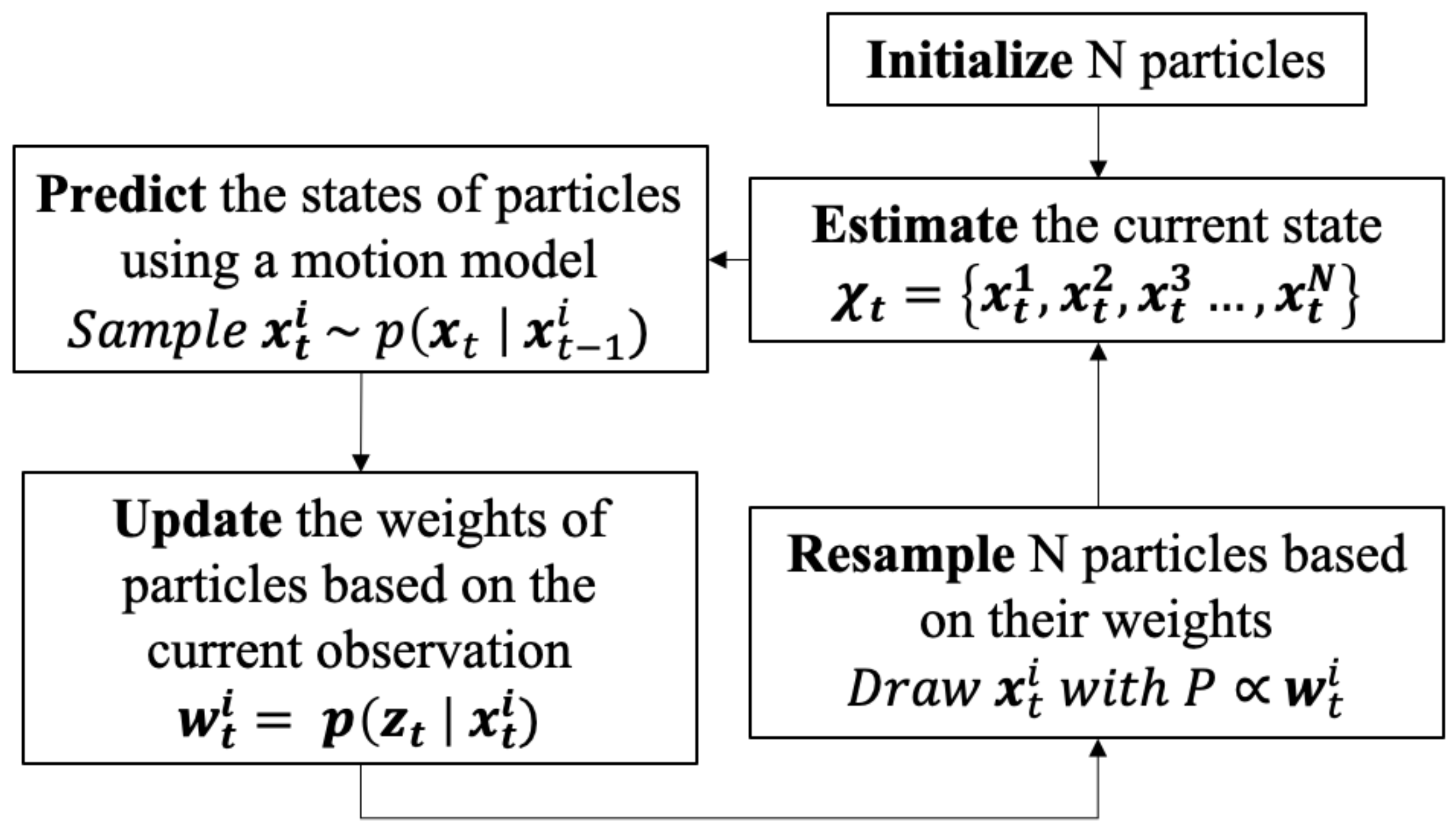
3.3. Particle-Filter-Based Occluded Vehicle Prediction

As pointed out in Section 3.1, the prediction of occluded vehicles is a crucial component of planning safe ego vehicle motion through blind intersections. In order to incorporate perception uncertainty and allow flexibility in the occluded vehicle behavior model in the prediction, we used a particle filter algorithm [32] in our model. The schematic diagram in Figure 6 illustrates the main steps of a basic particle filter algorithm.

The algorithm begins by generating a finite number of particles N, where a set of N particles at time t is denoted as follows:

$${\chi }_t=\{x_t^1,x_t^2,x_t^3,\dots ,x_t^N\}$$

(7)

Each particle $x_t^i$, when $1\le i\le N$, contains a state. In this study, a particle’s state represents a hypothesis of the state of an occluded vehicle at time t. Specifically, the state of each vehicle traveling on the intersecting roadway is represented by the state of a particle, which can be represented as follows:

$$x_t^i=\{s_t^i,ve{l}_t^i,a_t^i,A_t^i\}$$

(8)

where $s_t^i$ is the displacement from the current position of the particle to the intersection’s center, while $ve{l}_t^i$ and $a_t^i$ are the particle’s speed and acceleration, respectively. The last state variable, $A_t^i$, is a Boolean variable indicating whether the particle is aware of the ego vehicle.

After the particles are initialized, the current estimation of occluded vehicles’ state, ${\chi }_t$, is recursively updated at every time step $dt$, as a new observation becomes available. Starting from the previous estimated state, ${\chi }_{t-1}$, the current state of every particle is predicted using a motion model. The motion model used in this study is as follows:

$$\begin{array}{cc}\hfill s_t^i=& s_{t-1}^i+ve{l}_t^{i}dt+\frac{1}{2}{a}_t^{i}d{t}^2\hfill \\ \hfill ve{l}_t^i=& ve{l}_{t-1}^i+a_t^{i}dt\hfill \\ \hfill a_t^i=& f(s_{t-1}^i,ve{l}_{t-1}^i,A_t^i)\hfill \\ \hfill A_t^i=& \left\{\begin{array}{cc}True\hfill & ,\mathrm{if}{T}_{vis}^i\ge T_{react}\hfill \\ False\hfill & ,\mathrm{if}{T}_{vis}^i<T_{react}\hfill \end{array}\right.\hfill \end{array}$$

(9)

where $T_{vis}^i$ is the length of time the ego vehicle has been observable by the particle, which is determined by $s_t^i<V_{other}$. $T_{react}$ is a parameter that represents a recognition delay, i.e., the time it takes the approaching vehicle to become aware of the ego vehicle after it has become visible. The instantaneous acceleration of the particle, $a_t^i$, is determined by a function f, which, in this work, is designed to be dependent on the particle’s visibility of the ego vehicle in order to avoid a deadlock situation. This f function represents the visibility-dependent behavior of approaching vehicles, which will be discussed further in Section 4.

It is important to note that function f is not limited to only the behavior model proposed in this work, nor it is restricted to only one specific type of traffic participant. It can also be used to represent completely different behavior models, including the conventional approaching vehicle behavior model commonly used in blind intersection planners, i.e., a vehicle traveling toward the intersection at a certain constant speed can be expressed by a constant function, which outputs zero acceleration regardless of the state of the approaching vehicle. Moreover, the occluded object behavior function f can be applied to other types of traffic participants, e.g., pedestrians and bicycles.

After predicting the states of all the particles using the motion model, these particles represent samples drawn from a state transition distribution, $p\left(x_t\right|x_{t-1}^i)$. As observation $z_t$ becomes available, each particle is assigned an importance weight based on an observation model, $p\left(z_t\right|x_t^i)$. In this work, the Bernoulli distribution is used as our observation model:

$$p\left(z_t\right|x_t^i)=\left\{\begin{array}{c}\hfill 1-\alpha ,\phantom{-.}{s}_t^i<V_{ego}\\ \hfill \alpha ,\phantom{---}{s}_t^i\ge V_{ego}\end{array}\right.$$

(10)

where $\alpha$ represents the accuracy of the visible area classifier.

Lastly, a set of N particles is re-sampled based on their importance weights. These N particles now represent the current state estimate, ${\chi }_t$. All of the processes described above are then repeated at every time step.

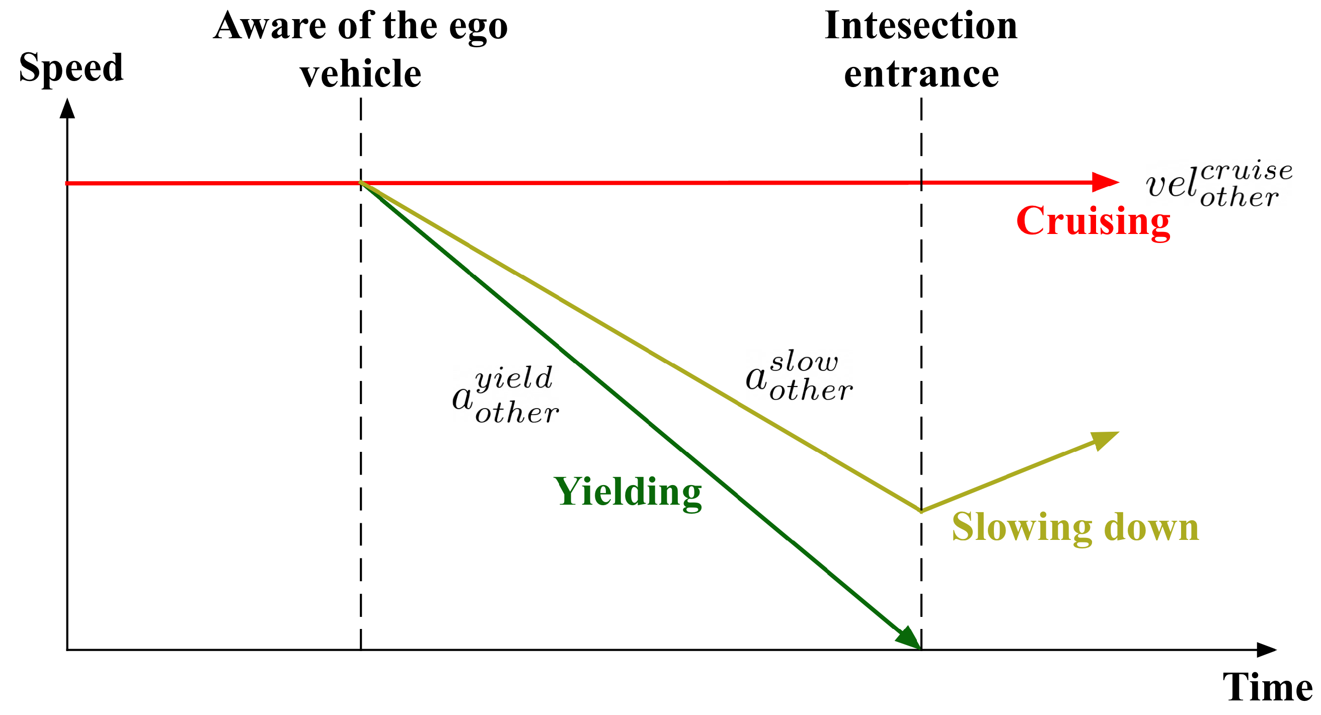
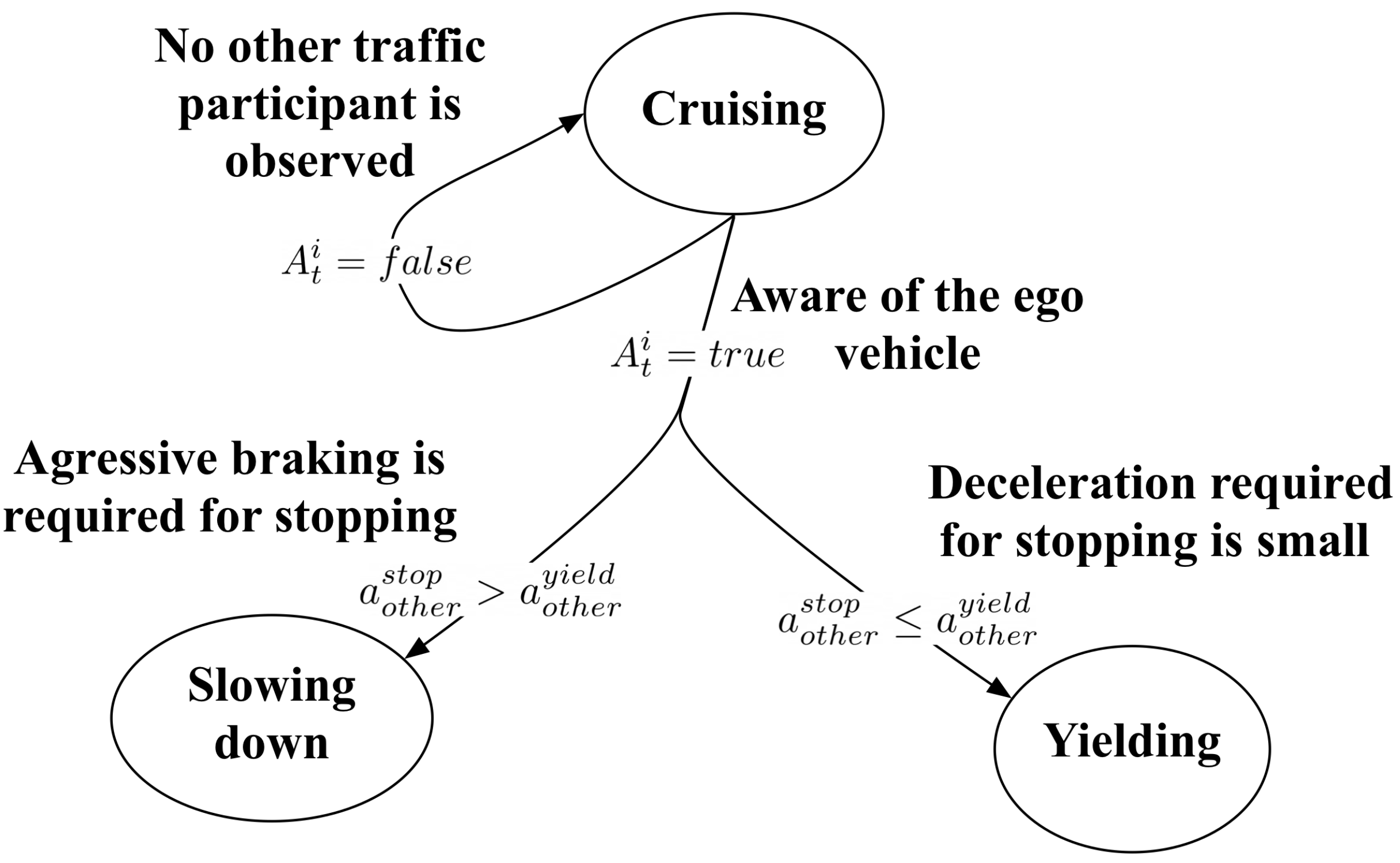
4. Proposed Visibility-Dependent Behavior Model for Approaching Vehicles

In order to address the occluded intersection deadlock problem, a more elaborate model for the behavior of approaching vehicles is proposed in this section. The proposed behavior model aims to capture possible changes in the behavior of approaching vehicles conditional on their visibility of the ego vehicle, i.e., a visibility-dependent behavior model. The proposed behavior model is incorporated into the particle-filter-based occluded vehicle prediction algorithm introduced in Section 3.3 via function f.

As the proposed behavior model is based on the analysis of collected real-world driving data, the details of data collection are given below in the first subsection. Subsequently, an analysis of the driving data is presented. Lastly, the proposed visibility-dependent behavior model is described.

4.1. Collection of Driving Data

It is essential to model the behavior of approaching vehicles in a way that represents the real behavior of actual drivers. In order to understand how drivers behave as they approach an intersection with limited visibility, driving data collected in such an environment are required. Therefore, an experiment was carried out to collect the required driving data, the details of which are described below.

4.1.1. Driver Types

Studies have shown that experienced and expert drivers tend to take proactive action to avoid collisions, e.g., by slowing down as they approach an intersection with poor visibility [19,33]. However, it is neither safe nor reasonable to assume that every driver approaching an intersection will behave in this manner. Therefore, our data collection experiment included the following different types of drivers in order to capture a wide range of driving behaviors at blind intersections:

• Expert drivers: Driving school instructors;
• Elderly drivers: Drivers who are 65 years old or older;
• Typical drivers: Drivers who do not belong to the other two groups.

A total of 18 drivers from these three different groups, including five male expert drivers, two female elderly drivers, two male elderly drivers, and four typical female drivers, participated in our data collection experiment.

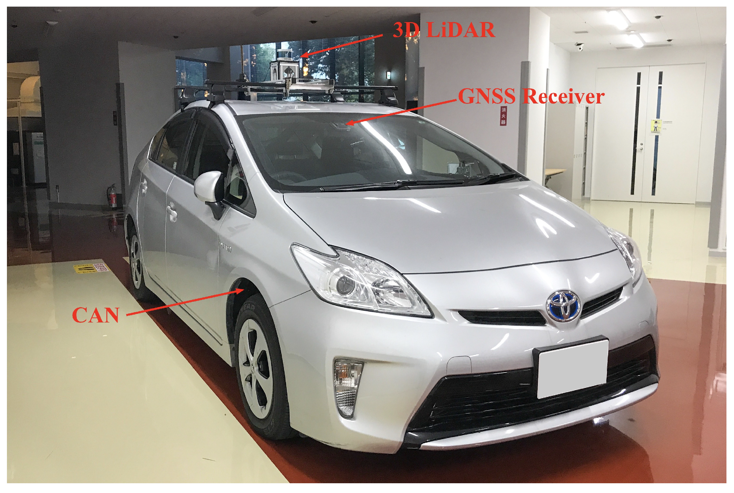
4.1.2. Experimental Vehicle

The vehicle used for data collection was the Toyota Prius shown in Figure 7. It was equipped with a 3D LiDAR sensor (Velodyne VLP-16) and a GPS receiver, which allowed real-time localization via the 3D Normal Distributions Transform (3D-NDT) scan-matching method proposed in [34]. Along with the previously mentioned sensors, the Controller Area Network (CAN) data, which included speed and brake pressure, were also collected. By fusing data from different sensors, the position, orientation, and speed of the vehicle at each location could be obtained.

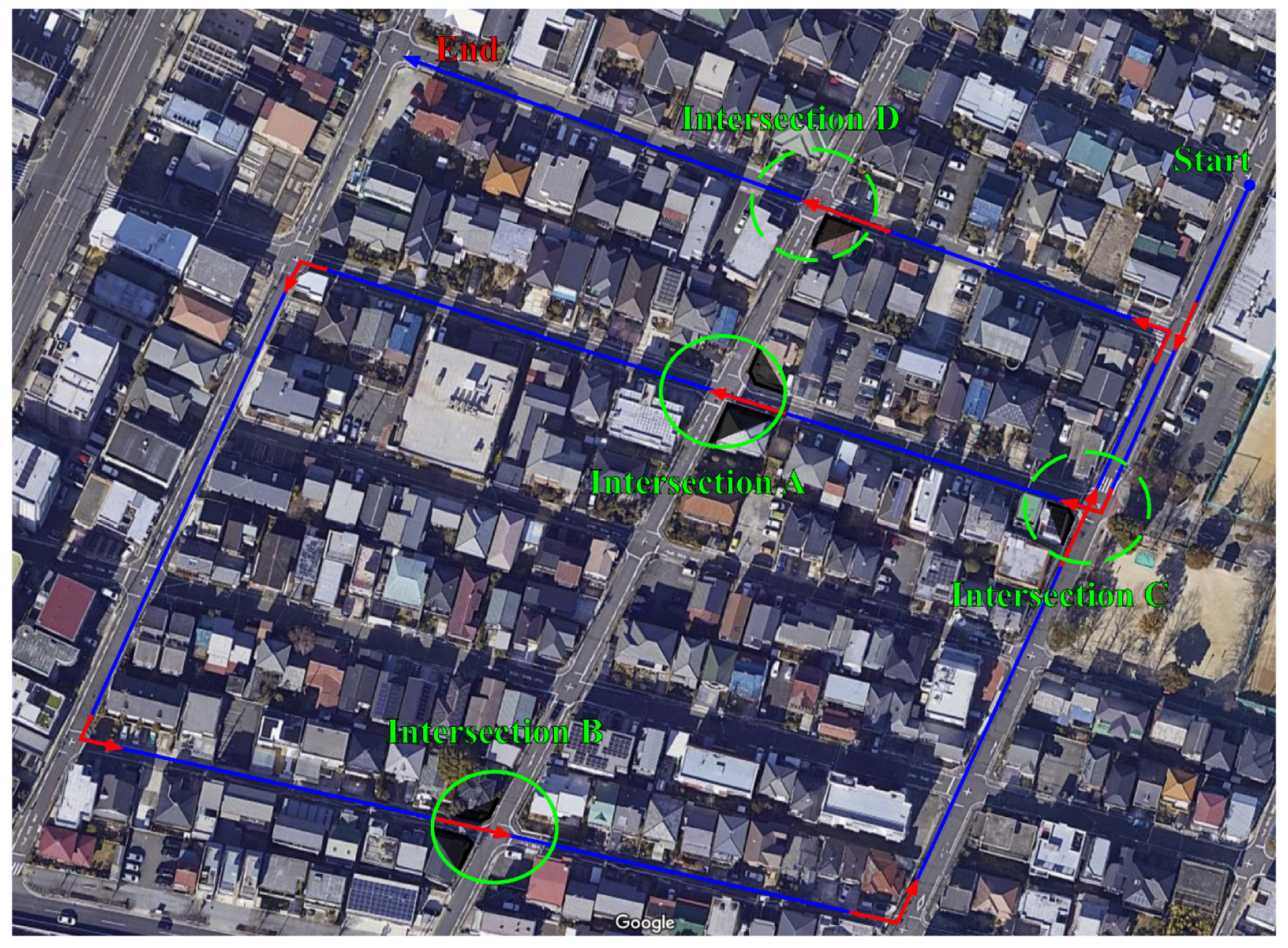
4.1.3. Experimental Environment

The environment selected for data collection was a residential area of Nagoya, Japan, which contained several intersections without traffic signals that had notably low visibility. The driving route for data collection is shown in Figure 8. From the beginning to the end of the route, each driver crossed a total of four blind intersections. Two of the intersections required drivers to make a mandatory stop, namely, intersections A and B, while the other two, intersections C and D, did not require drivers to stop prior crossing (a satellite view of the experimental environment and driving route can be found at: https://drive.google.com/open?id=1CbrP0BYfK0tPR_Qs60Qkjov-PJDk3pEK&usp=sharing (accessed on 26 December 2020)).

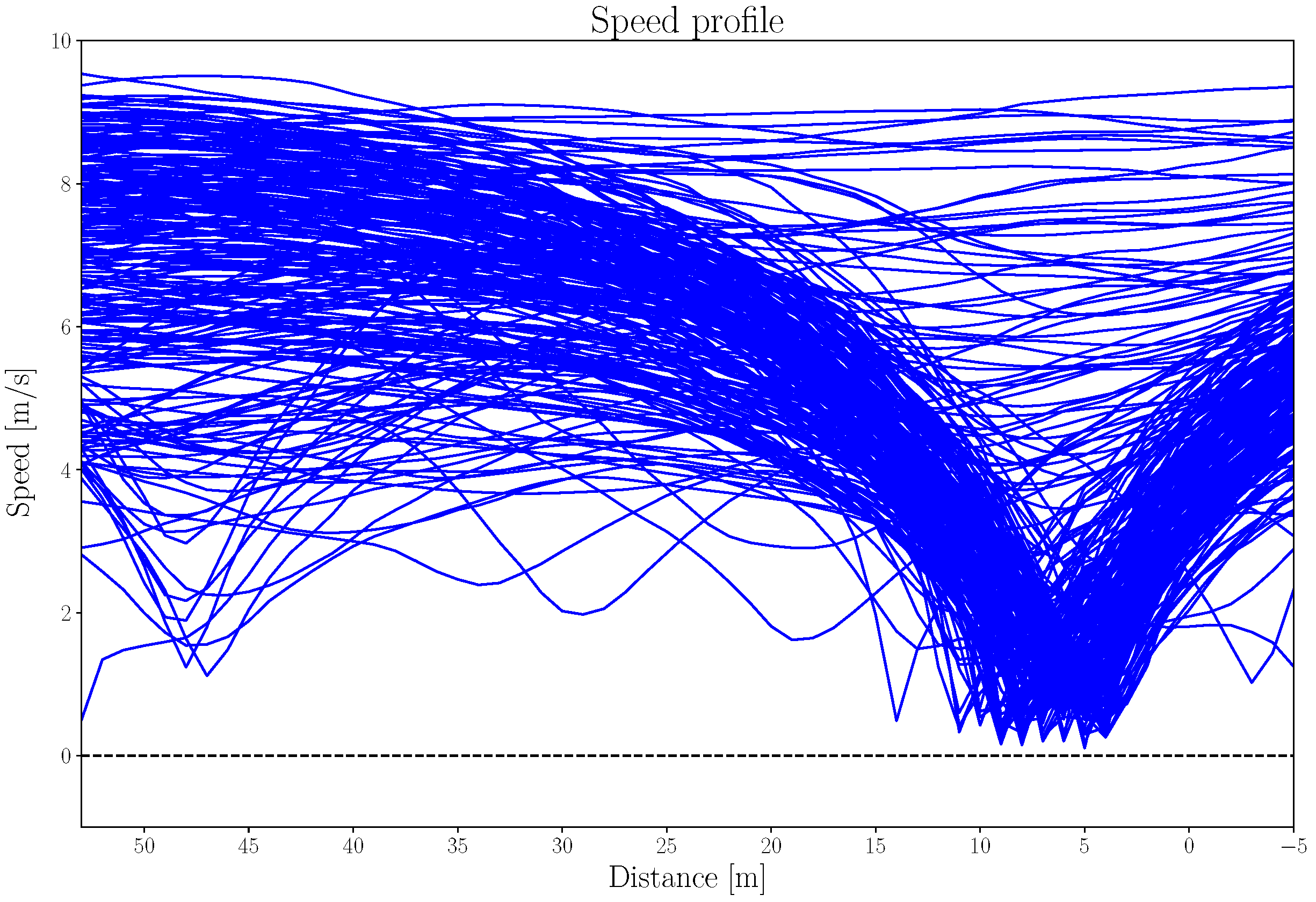
4.2. Driving Data Analysis

Data from a total of 232 intersection crossings by 18 drivers were collected. In order to visualize all of the crossing data from the various intersections in one graph, the distance from the center of each intersection to the experimental vehicle was used to represent the location of the vehicle. Profiles of crossing speeds at the selected blind intersections are shown in Figure 9. We can see that most of the drivers initially approached the intersections at a speed of approximately 8 m/s, which is just below the local speed limit, i.e., 8.33 m/s or 30 km/h. Moreover, the data in Figure 9 show that the majority of drivers slowed down as they approached the intersections. In some cases, however, drivers maintained a relatively high speed as they crossed the intersection. The data suggest that there are a variety of possible behaviors when vehicles are approaching blind intersections.

In order to further analyze the behavior of the approaching vehicles, cluster analysis was performed. The K-Mean clustering algorithm [35] was used to group similar speed profiles into clusters. The optimal number of clusters, which is the main parameter of the K-Mean clustering algorithm, was determined based on the silhouette coefficient [36]. As a result, the speed profiles were divided into three groups. The average speed at each location in relation to the intersection, i.e., the average speed profile, for each of the three clusters is represented by the red, yellow, and green lines in Figure 10. The standard deviation of vehicle speed at each location for each cluster is represented by a vertical band.

As indicated by the red profile in Figure 10, cruising through intersections at a constant speed appears to be one of the behaviors of approaching vehicles. The yellow and green profiles in Figure 10 both show approaching vehicles slowing down prior to a blind intersection. However, the green profile reaches a lower minimum speed compared to the yellow profile.

4.3. Proposed Visibility-Dependent Behavior Model

Based on our analysis of the collected data, here, we propose a behavior model for vehicles approaching blind intersections. The proposed model consists of three possible behaviors, namely, Cruising, Slowing down, and Yielding. These behaviors correspond to the red, yellow, and green speed profiles shown in Figure 10, respectively.

Our ultimate goal when designing the approaching vehicle behavior model was to use it for defining function f in the particle-filter-based occluded vehicle prediction. As the function f is used for estimating the instantaneous acceleration of occluded vehicles, a speed profile for each behavior in the time domain is required. Therefore, we next modeled a speed profile for each type of intersection approaching behavior, and these speed profiles are shown in Figure 11. For the Cruising profile, the vehicle approaches and crosses the intersection at a constant speed of $ve{l}_{other}^{cruise}$, resulting in zero acceleration the entire time. As for the Slowing down profile, the vehicle also travels toward the intersection at a speed of $ve{l}_{other}^{cruise}$ initially. However, at some point, it starts to decelerate at a rate of $a_{other}^{slow}$, before accelerating again to cross the intersection. Lastly, the Yielding profile represents behavior similar to Slowing down, but the vehicle slows down to a full stop prior to the intersection from an initial speed of $ve{l}_{other}^{cruise}$. Apart from the minimum speed before crossing the intersection, another difference between the Yielding and Slowing down profiles is the rate at which the vehicles slow down. For the Yielding profile, the approaching vehicle applies a relatively sharper deceleration of $a_{other}^{yield}$ in order to come to a full stop before the intersection.

Furthermore, we propose that these behaviors are connected, and that transitions between them can be explained by whether or not the driver detects another traffic participant on the intersecting road and by the deceleration required to yield after detecting another vehicle. These transitions are represented in the form of a diagram in Figure 12. As can be seen in the diagram, an approaching vehicle starts in the Cruising state, i.e., traveling toward an intersection at a constant speed of $ve{l}_{other}^{cruise}$. When no traffic participant is observed on the intersecting roadway, the approaching vehicle remains in the same state. The transition from Cruising behavior occurs when the driver of the approaching vehicle becomes aware of the ego vehicle on the intersecting roadway, i.e., when $A_t^i$ is true, since the ego vehicle has become observable for a period of at least $T_{react}$. This transition results in Yielding if the amount of deceleration required to come to a full stop, $a_{other}^{stop}$, does not exceed a limit of $a_{other}^{yield}$. Otherwise, the behavior switches from Cruising to Slowing down, as the driver would have to decelerate too abruptly to stop.

This proposed behavior model can be viewed as a more elaborate extension of the worst-case-scenario behavior model commonly used in related studies, where occluded vehicles are assumed to maintain a constant speed regardless of the situation, since it provides a behavior transition from worst-case-scenario behavior, i.e., Cruising, to other behaviors that can be observed in real traffic. Even though the proposed behavior transitions are deterministic and only conditioned on two factors, namely, observation of other traffic participants and the amount of deceleration required for stopping, they can be further extended to probabilistic transitions that are conditioned on other factors, e.g., the probability of an approaching vehicle changing its state from Cruising to Yield could be set higher in situations where it is traveling toward an intersection with a mandatory stop.

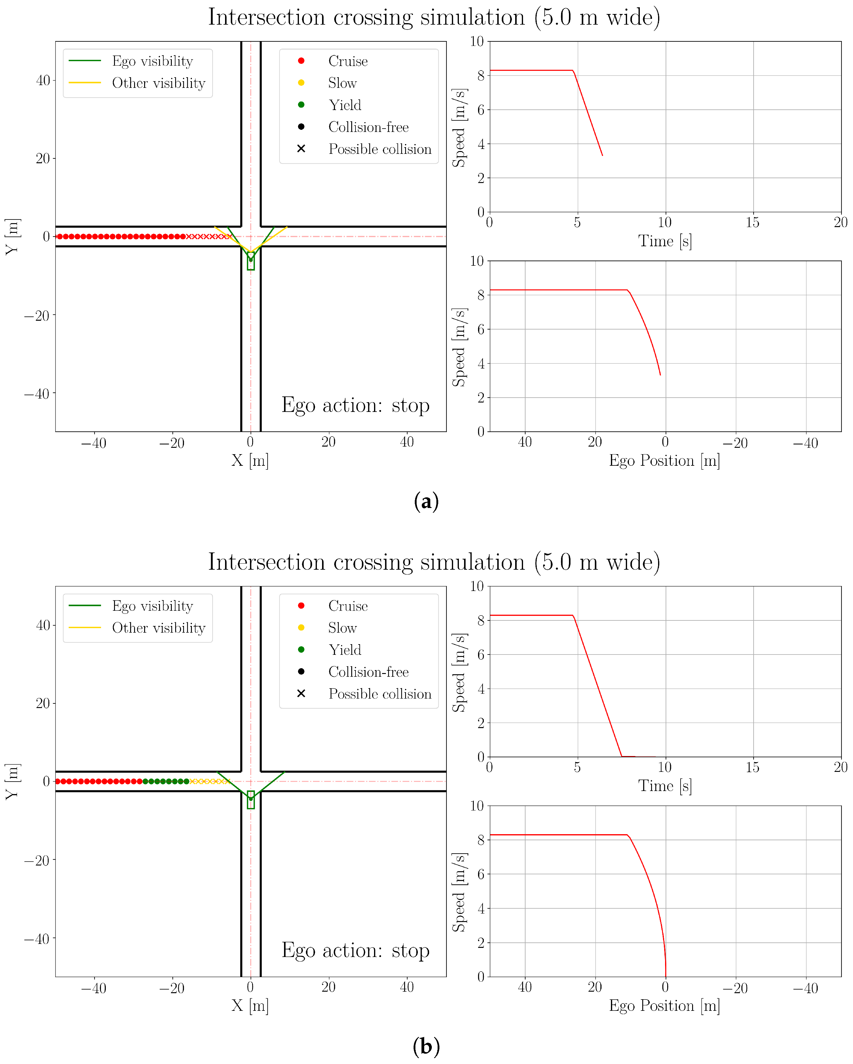
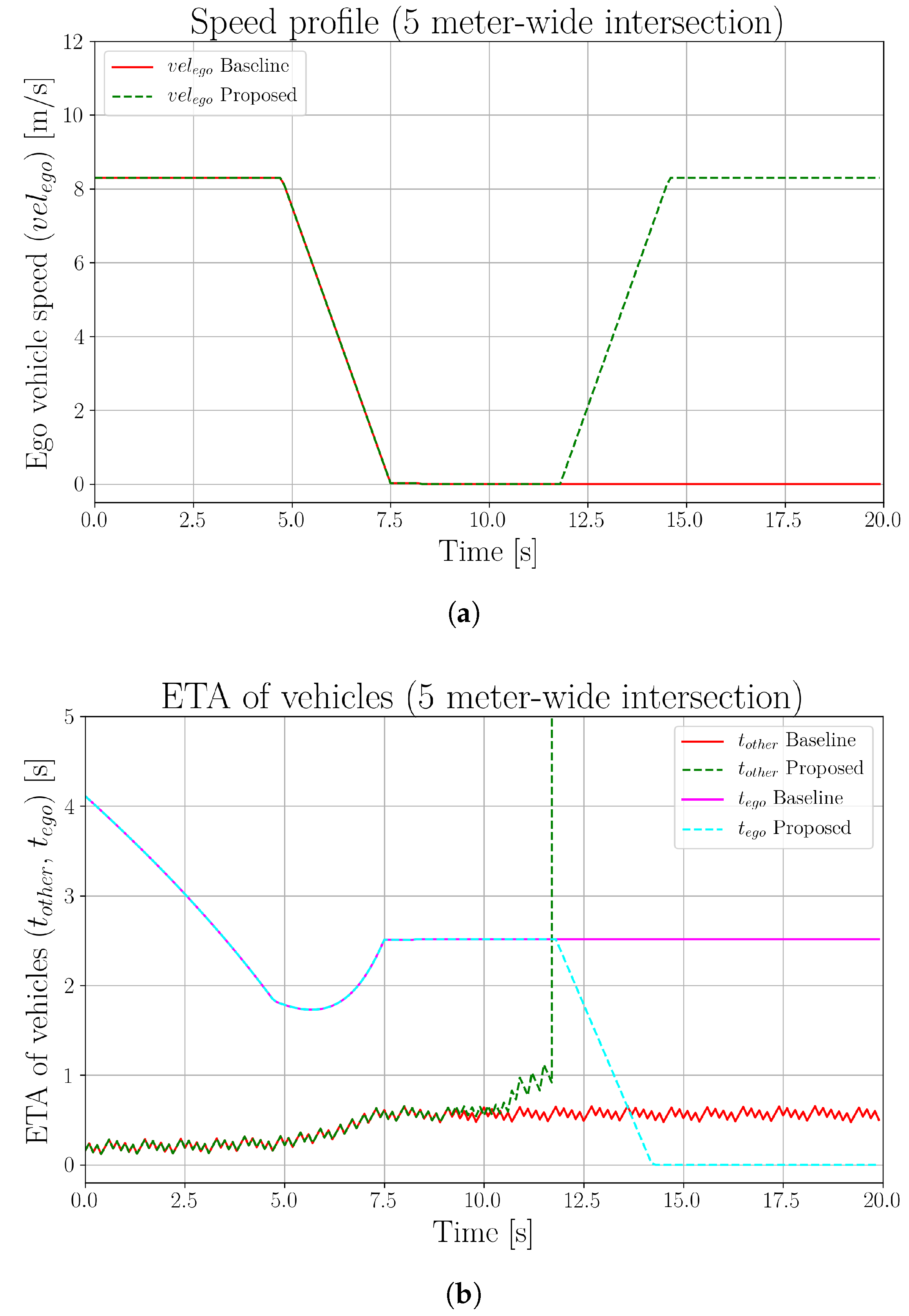
5. Experimental Results

In order to validate the performance of the proposed intersection crossing planner at occluded intersections, a closed-loop intersection crossing simulator was developed. The simulation allowed us to test the proposed planner under various visibility conditions and sensor configurations while maintaining other factors that could affect the output motion. Figure 13 shows outputs of the closed-loop simulator, illustrating the operation of the proposed planner during an intersection crossing event. The simulation begins with the ego vehicle 50 m from the intersection’s entrance, traveling toward the intersection at the maximum speed of 8.3 m/s. At each time step, the simulator uses the output acceleration from the proposed planner to compute the ego vehicle’s speed and position at the next time step. These processes are then repeated every 0.1 s until the simulation times out after 20 s.

Three different experiments were carried out in order to highlight the different characteristics of the proposed planner (videos of our experiment can be found at: https://youtu.be/Bic2QL2RQps (accessed on 26 December 2020)). In each experiment, the planner was tested at two intersections with different visibility conditions, i.e., at intersections of roads that were both either 5 m or 15 m wide. The major parameters used in these simulation experiments are summarized in

Table 1. Values of major parameters used in the experiments.

Parameter	Value	Parameter	Value
$L_{ego}$	4.5 m	$Widt{h}_{ego}$	1.7 m
$W_{ego}$	5.0, 15.0 m	$W_{cross}$	5.0, 15.0 m
$a_{ego}^{cross}$	3.0 m/s${}^2$	$a_{ego}^{stop}$	−3.0 m/s${}^2$
$a_{other}^{yield}$	−1.5 m/s${}^2$	$a_{other}^{slow}$	−0.8 m/s${}^2$
$ve{l}_{other}^{cruise}$	8.3 m/s	$T_{react}$	2.3 s

.

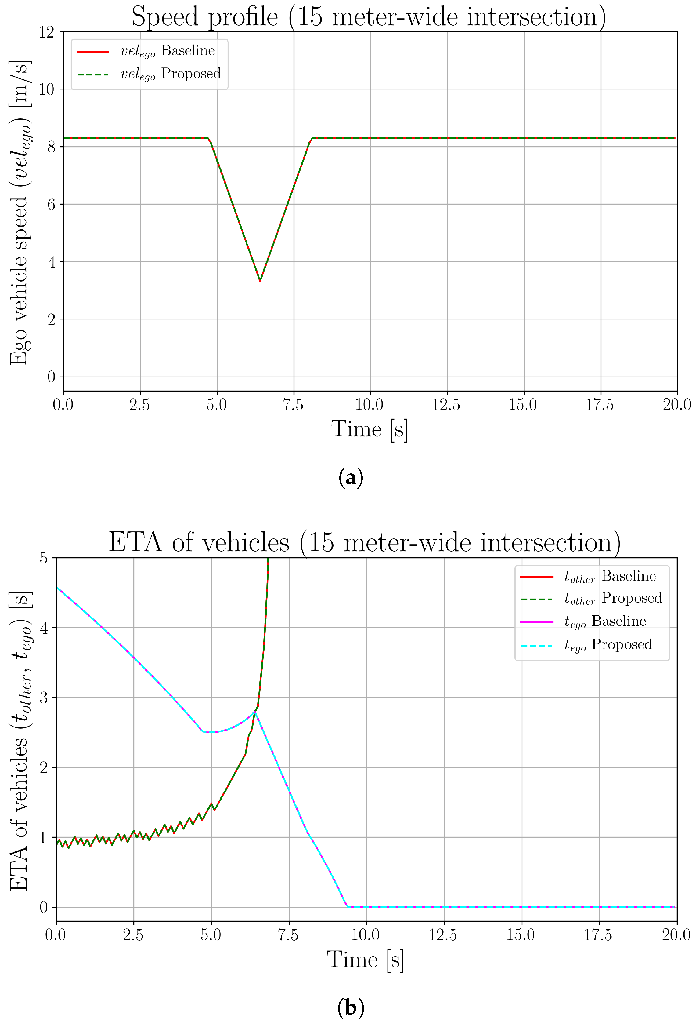
5.1. Baseline Comparison

An initial experiment was carried out to verify the effectiveness of the visibility-dependent behavior model for approaching vehicles in solving the deadlock problem. The proposed planner was compared with a baseline model that assumed that an occluded vehicle was approaching the intersection at a constant speed from outside the area visible to the ego vehicle. In this experiment, the sensor was mounted 2 m from the front end of the ego vehicle, i.e., $X_{sensor}=2$ m. Moreover, perception accuracy was set to be 100%, i.e., $\alpha =1.0$.

Figure 13 shows a sequence of ego vehicle motions generated by the proposed planner at a 5 m wide blind intersection. The hypothetical occluded vehicles (or “particles”) are depicted with either a × (representing a possible collision) or • (representing a collision-free crossing) depending on whether or not they will reach the overlapping zone of the intersection before the ego vehicle finishes crossing, i.e., $t_{ego}\ge t_{other}$ or $t_{ego}<t_{other}$, respectively. The color of these particles indicates their current behavior; green represents Yield behavior, yellow represents Slowing down behavior, and red represents Cruise behavior.

As can be seen in Figure 13a, the ego vehicle slowed down as it approached the intersection, since its visibility, shown by the green lines, was very limited. Similarly, the ego vehicle was observable by vehicles approaching on the intersecting roadway only from a position very close to the intersection, i.e., after entering the area between the two yellow lines. As depicted in Figure 13b, the ego vehicle came to a full stop at the entrance to the intersection. From this position, the ego vehicle’s visibility was still insufficient for crossing. However, the ego vehicle could be observed by approaching vehicles from a more distant location, as its front end was now aligned with the corner. Therefore, some of the particles started to change their behavior from Cruising to Slowing down or Yield, depending on their position. As shown in Figure 13c, once the ego vehicle stopped at the intersection for some time, all of the particles close to the intersection changed their behavior to Yield. Consequently, the ego vehicle began crossing the intersection, as the safe crossing condition defined in Equation (1) was satisfied, as shown in Figure 13d. As a result of proceeding forward, the ego vehicle gained more visibility along the intersecting roadway, causing the hypothetical occluded vehicles to be eliminated.

The proposed planner’s speed profile for crossing a 5 m wide intersection is represented by the dashed green line in Figure 14a. We can see that the ego vehicle reduces its speed constantly until reaching a full stop. It then remains at rest for a few seconds before starting to accelerate again.

As for the baseline planner, its speed profile is depicted by the solid red line in Figure 14a. When approaching the intersection, the baseline and proposed planners generated identical motion; therefore, the two speed profiles overlap perfectly. However, after the ego vehicle comes to a full stop, the baseline planner does not generate any crossing motion command due to insufficient visibility. Consequently, the ego vehicle remains in a deadlocked situation until the simulation times out.

Next, the estimated times of arrival for the ego vehicle, $t_{ego}$, and of the predicted occluded vehicle, $t_{other}$, for both the baseline and proposed planners are shown in Figure 14b. The green and cyan dashed lines represent $t_{ego}$ and $t_{other}$ as estimated by the proposed planner, respectively. Initially, $t_{other}$ was extremely low, and it remainde almost unchanged. Meanwhile, $t_{ego}$ constantly decreased as the ego vehicle approached the intersection at a constant speed. Since $t_{ego}$ remained larger than $t_{other}$, the ego vehicle began braking. As the ego vehicle’s speed fell, $t_{ego}$ decreased at a slower rate before beginning to increase again as the vehicle slowed to a full stop. At the full stop, $t_{ego}$ remained constant, while $t_{other}$ began to increase after a few seconds as the particles began to adjust their speed. The increasing $t_{other}$ eventually surpassed the constant $t_{ego}$, allowing the ego vehicle to begin crossing the intersection. As the ego vehicle crossed the intersection, $t_{ego}$ began to drop until it finally reached zero once the crossing was completed.

For the baseline planner, the plots of $t_{ego}$ and $t_{other}$ were identical to those for the proposed planner prior to the full stop, as shown in Figure 14b. In contrast to the proposed planner, however, $t_{other}$ as well as $t_{ego}$ remained almost unchanged after the stop, causing the gap between them to remain nearly constant. As $t_{other}$ never exceeded $t_{ego}$, the ego vehicle continued to be trapped in a deadlock until the end of the simulation.

We also compared the two planners at an intersection with relatively better visibility, i.e., at an intersection of two roads that are 15 m wide. As shown in Figure 15a, the output speed profiles of both planners were identical. Initially, the ego vehicle approaches the intersection at a constant speed, and then it starts to slow down in order to prepare for a stop prior to the intersection. However, as it approaches the intersection, the ego vehicle starts to accelerate and crosses the intersection without stopping.

Similarly, the estimated $t_{other}$ and $t_{ego}$ of the proposed and baseline planners are indistinguishable, as can be seen in Figure 15b. As the ego vehicle progresses toward the intersection at a constant speed, $t_{ego}$ gradually declines, while $t_{other}$ increases at an accelerating rate. Even though $t_{ego}$ starts to rise due to braking, the ego vehicle’s visibility increases exponentially as the ego vehicle reaches the intersection, and $t_{other}$ eventually exceeds $t_{ego}$. This is the moment at which the ego vehicle starts to accelerate to cross the intersection.

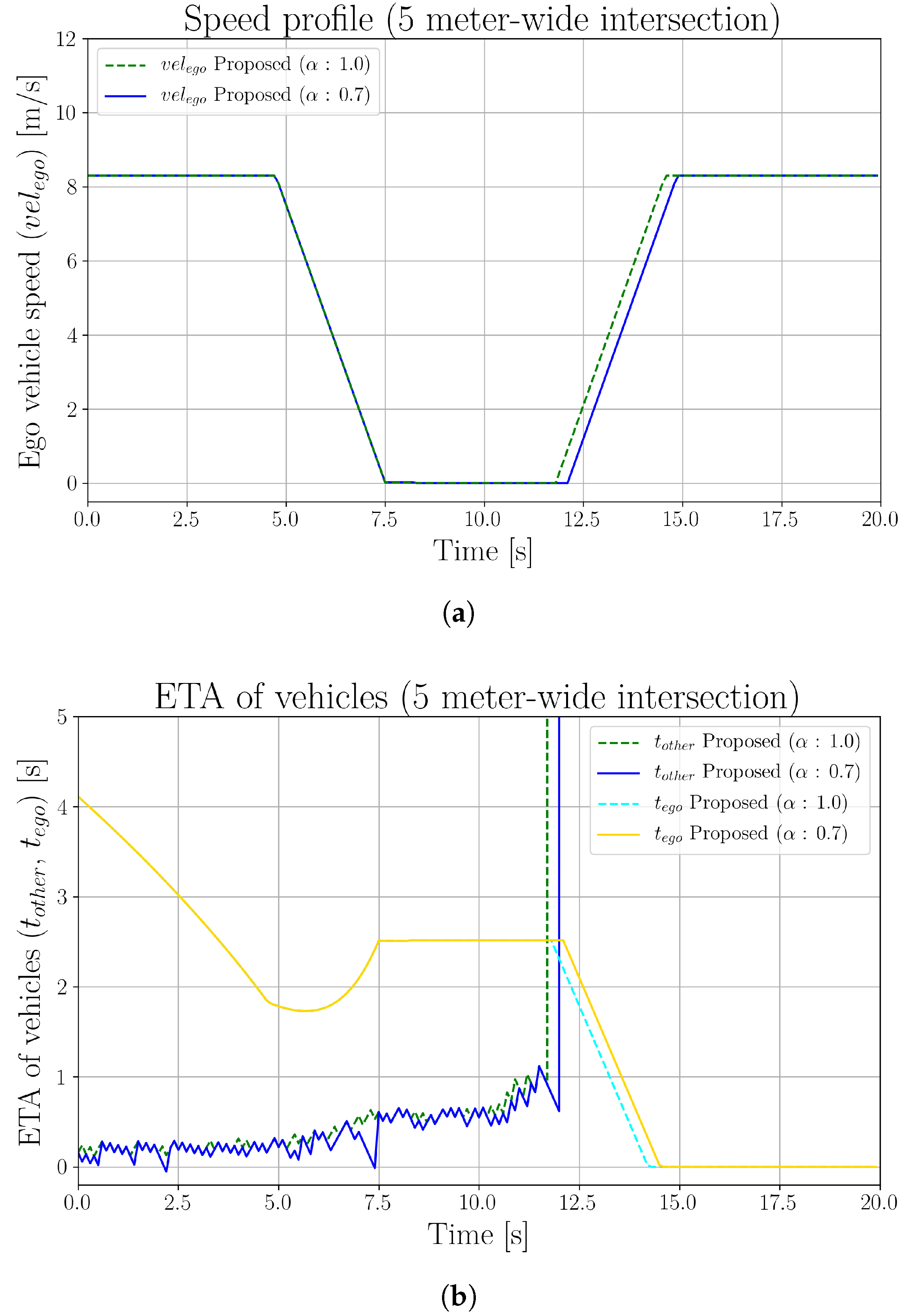
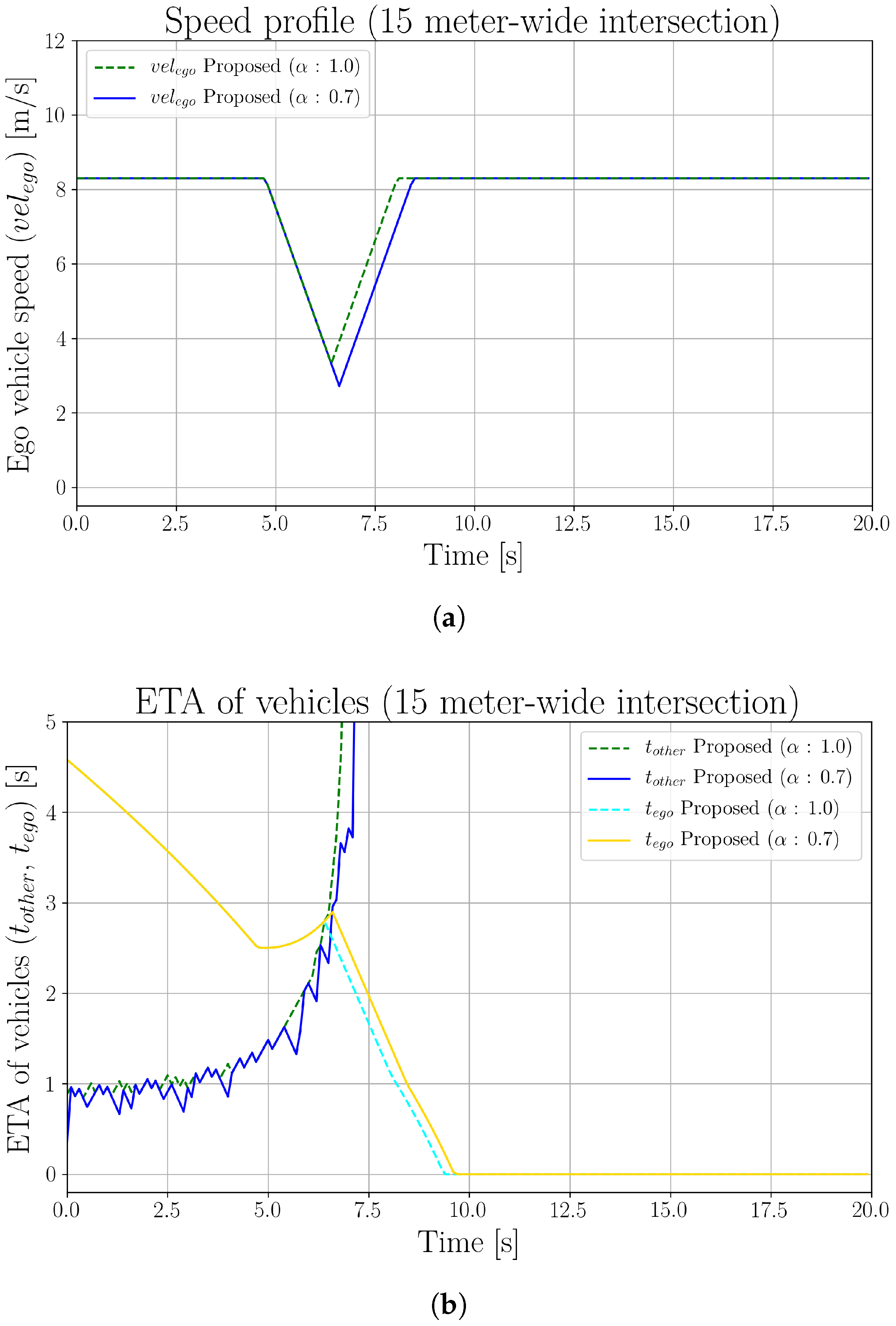
5.2. Effects of Perception Inaccuracy

As mentioned in Section 3.3, the proposed planner utilizes a particle filter algorithm for occluded vehicle prediction in order to account for uncertainty from the perception module. This experiment aims to investigate how perception inaccuracy affects the output motion of the proposed planner. The proposed planner was tested with occluded intersections of both 5 m and 15 m wide roadways using two different perception accuracy values ($\alpha$ = 1.0 and $\alpha$ = 0.7), while $X_{sensor}$ was set to 2 m, representing the location of a rooftop-mounted LiDAR unit.

When encountering an intersection of 5 m wide roads, the speed profiles shown in Figure 16a indicate that, overall, the output motion of the proposed planner is similar regardless of which $\alpha$ value is used. More specifically, the ego vehicle slowed down and came to a full stop prior to the intersection. After a few seconds of waiting at the entrance to the intersection, the ego vehicle finally began crossing it. However, in the case of imperfect perception, i.e., when $\alpha =0.7$, the ego vehicle stayed at rest slightly longer before it started crossing the intersection compared to the scenario when $\alpha =1.0$, i.e., perfectly accurate perception.

The effect of noisy perception is evident in Figure 16b. The estimated time of arrival of an occluded vehicle, $t_{other}$, appears to fluctuate more when $\alpha =0.7$. Moreover, $t_{other}$ began exceeding $t_{ego}$ later than when the perception was ideal.

Figure 17a shows the resulting speed profiles for both perception accuracy settings at an occluded intersection of roads with a width of 15 m. The output motions at both settings are similar, i.e., the ego vehicle slows down before crossing the intersection without stopping. While both settings output similar motions, with $\alpha$ set to 0.7, the proposed planner generated a lower minimum speed and a more delayed crossing action than when $\alpha =1.0$. Furthermore, as shown in Figure 17b, the estimate of $t_{other}$ is noisier when the perception is imperfect.

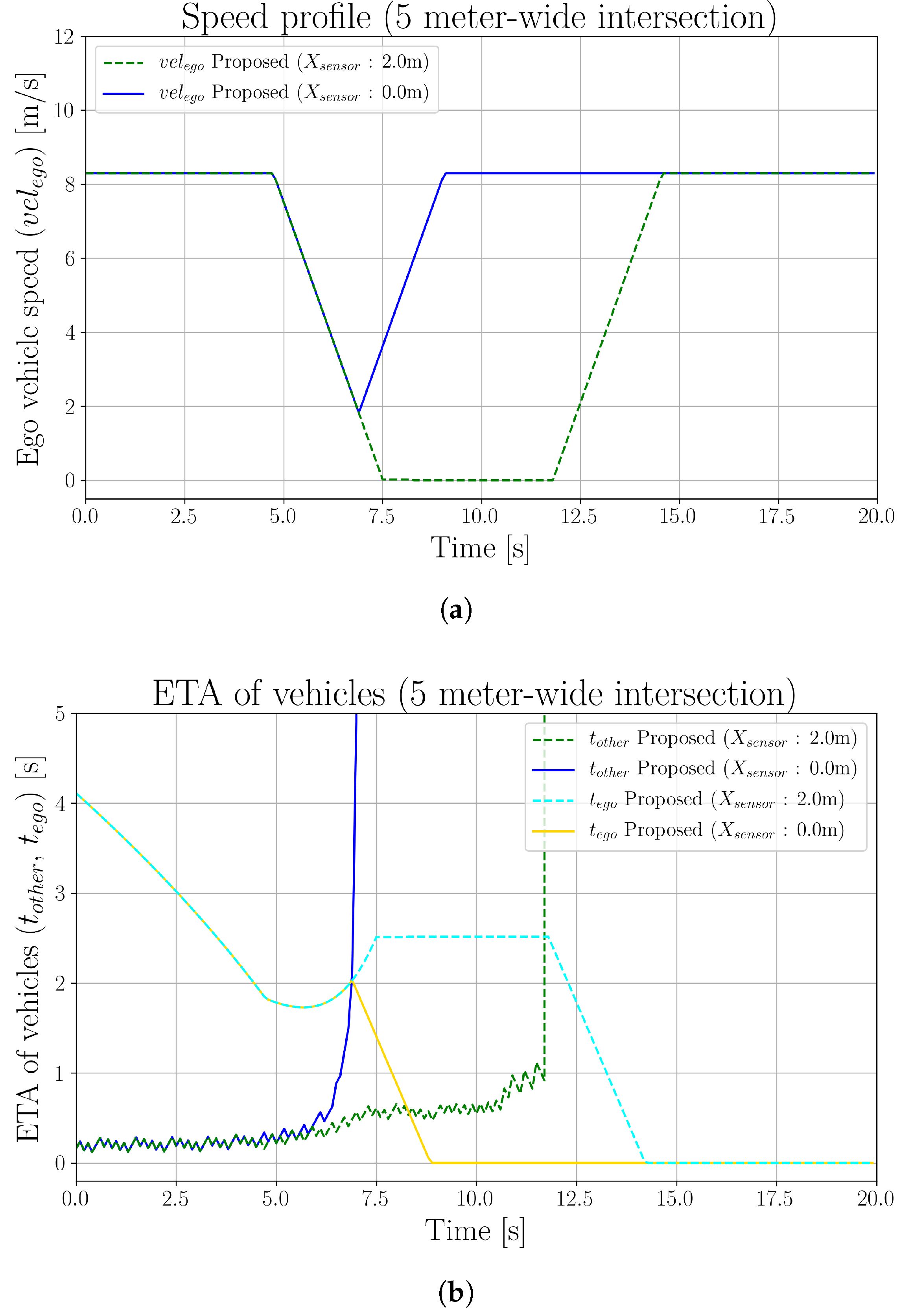
5.3. Effects of Sensor Mounting Position

As described in Section 3.2, one of the factors that significantly affects the ego vehicle’s visibility at blind intersections is the sensor mounting position, $X_{sensor}$. The purpose of the next experiment was to examine the effects of the sensor mounting position on the output motions of the proposed planner.

Two sensor positions were tested in this experiment. The sensor was either mounted close to the vehicle’s center, i.e., $X_{sensor}=2.0$ m, which is consistent with a rooftop-mounted LiDAR unit, or the sensor was simulated to be mounted at the front of the vehicle, i.e., $X_{sensor}=0.0$ m, consistently with a front-bumper-mounted sensor. In both cases, $\alpha$ was set to 1.0, representing perfect perception.

As can be seen in Figure 18a, the output speed profiles are clearly different when the intersecting roads are 5 m wide. The green dashed line shows that the ego vehicle came to a full stop and waited before crossing the intersection when the sensor was mounted close to the vehicle’s center, i.e., $X_{sensor}=2.0$ m. On the contrary, as illustrated by the solid blue line, the ego vehicle slowed down until it reached the minimum speed of 1.82 m/s before crossing the intersection without stopping when the sensor was mounted at the front of the ego vehicle.

Variation in the outputs of the proposed planner with different sensor mounting positions can also be observed in Figure 18b. When the sensor was front-mounted, $t_{other}$ increased rapidly as the ego vehicle was about to reach the entrance of the intersection, as depicted by the blue line. Meanwhile, $t_{other}$ remained nearly unchanged when using the center-mounted configuration.

At an intersection with relatively better visibility, i.e., an intersection of two 15 m wide roads, the output speed profiles of the two configurations are more similar, as can be seen in Figure 19a. In both cases, the ego vehicle slowed down to a certain speed before accelerating again and continuing through the intersection. However, when the sensor was mounted close to the center of the ego vehicle, the vehicle decelerated until it reached the minimum speed of 3.32 m/s, which is 1.50 m/s lower compared to the lowest speed before crossing in the case of front-mounted configuration.

Despite slight variations in timing between the increase in $t_{other}$ and $t_{ego}$, depending on the location of the sensor unit, the motion planning output for both sensor positions are very similar, as shown in Figure 19b.

6. Conclusions

In this study, we proposed a generic deadlock-free motion planner that utilizes both ego and approaching vehicles’ visibility to generate safe crossing motion at blind intersections. In order to support possible changes in the behavior of approaching traffic participants based on their ability to see the ego vehicle, and to account for uncertainty in perception accuracy, the proposed planner utilizes a particle filter algorithm for occluded vehicle prediction. For modeling the visibility-dependent behavior of occluded vehicles at intersections, real driving data from multiple drivers crossing blind intersections in a residential area were collected and analyzed. Based on our analysis of the behavior of occluded vehicles when approaching intersections, the model of the behavior of approaching vehicles, which depends on their visibility of the ego vehicle, was introduced.

To validate the ability of our proposed method to overcome the deadlock problem at blind intersections, the proposed planner was compared with a baseline planner that simply assumed that other vehicles were approaching from the occluded area at a constant speed. Our comparison of the proposed and baseline planners in a simulation experiment showed that the proposed planner could generate deadlock-free crossing motion at a blind intersection of two narrow roads (each 5 m wide), while the baseline planner could not. The effects of perception accuracy and sensor position on the output motion of the planner were also investigated. As for the effects of noisy perception, it was found that inaccuracy in perception generally caused the proposed planner to slightly delay intersection crossing action. Furthermore, it was found that the sensor mounting position significantly affected the output of the proposed planner at intersections of narrow roadways (each 5 m wide) with poor visibility. When the sensor was mounted at the front of the ego vehicle, the vehicle slowed down, but did not stop prior to crossing the intersection. In contrast, when a center-mounted sensor configuration was used, the ego vehicle slowed to a complete stop before it started crossing the intersection.

It is important to note that, while closed-form expressions were used in this work to estimate visibility at a blind intersection, a more sophisticated approach for estimating visibility, such as the one used in our previous work [11], can be used as a substitution to enable the proposed planner to deal with complex real-world environments.

Even though this study only considers potential occluded vehicles, other types of traffic participants, such as pedestrians and cyclists, can be integrated into the occluded object prediction by properly defining their behavior models. Moreover, as the proposed planner offers an approach for considering potential behavior changes of occluded traffic participants, it could be extended to cover other situations where more than one single behavior of occluded objects is possible. For example, it could be used to model a possible deceleration of an occluded approaching cyclist after the ego vehicle gives an audible warning with the horn. Additionally, the concept of behavior change of occluded objects can be utilized in the POMDP framework to solve for the optimal action in more complex scenarios.

References

1. Singh, S. Critical Reasons for Crashes Investigated in the National Motor Vehicle Crash Causation Survey; Technical Report; NHTSA’s National Center for Statistics and Analysis: Washington, DC, USA, 2018.
2. Fagnant, D.J.; Kockelman, K. Preparing a nation for autonomous vehicles: Opportunities, barriers and policy recommendations. Transp. Res. Part A Policy Pract. 2015, 77, 167–181. [Google Scholar] [CrossRef]
3. Wadud, Z.; MacKenzie, D.; Leiby, P. Help or hindrance? The travel, energy and carbon impacts of highly automated vehicles. Transp. Res. Part A Policy Pract. 2016, 86, 1–18. [Google Scholar] [CrossRef] [Green Version]
4. Chan, C.Y. Advancements, prospects, and impacts of automated driving systems. Int. J. Transp. Sci. Technol. 2017, 6, 208–216. [Google Scholar] [CrossRef]
5. Yurtsever, E.; Lambert, J.; Carballo, A.; Takeda, K. A Survey of Autonomous Driving: Common Practices and Emerging Technologies. IEEE Access 2020, 8, 58443–58469. [Google Scholar] [CrossRef]
6. González, D.; Pérez, J.; Milanés, V.; Nashashibi, F. A Review of Motion Planning Techniques for Automated Vehicles. IEEE Trans. Intell. Transp. Syst. 2016, 17, 1135–1145. [Google Scholar] [CrossRef]
7. Geissler, F.; Grafe, R. Optimized sensor placement for dependable roadside infrastructures. In Proceedings of the 2019 IEEE Intelligent Transportation Systems Conference (ITSC 2019), Auckland, New Zealand, 27–30 October 2019; pp. 2408–2413. [Google Scholar] [CrossRef] [Green Version]
8. Zhao, X.; Wang, J.; Yin, G.; Zhang, K. Cooperative Driving for Connected and Automated Vehicles at Non-signalized Intersection based on Model Predictive Control. In Proceedings of the 2019 IEEE Intelligent Transportation Systems Conference (ITSC 2019), Auckland, New Zealand, 27–30 October 2019; pp. 2121–2126. [Google Scholar] [CrossRef]
9. Hafner, M.R.; Cunningham, D.; Caminiti, L.; Del Vecchio, D. Cooperative collision avoidance at intersections: Algorithms and experiments. IEEE Trans. Intell. Transp. Syst. 2013, 14, 1162–1175. [Google Scholar] [CrossRef]
10. Milanés, V.; Villagrá, J.; Godoy, J.; Simó, J.; Pérez, J.; Onieva, E. An intelligent V2I-based traffic management system. IEEE Trans. Intell. Transp. Syst. 2012, 13, 49–58. [Google Scholar] [CrossRef] [Green Version]
11. Narksri, P.; Takeuchi, E.; Ninomiya, Y.; Takeda, K. Crossing Blind Intersections from a Full Stop Using Estimated Visibility of Approaching Vehicles. In Proceedings of the 2019 IEEE Intelligent Transportation Systems Conference (ITSC 2019), Auckland, New Zealand, 27–30 October 2019; pp. 2427–2434. [Google Scholar] [CrossRef]
12. Brechtel, S.; Gindele, T.; Dillmann, R. Probabilistic decision-making under uncertainty for autonomous driving using continuous POMDPs. In Proceedings of the 2014 17th IEEE International Conference on Intelligent Transportation Systems (ITSC 2014), Qingdao, China, 8–11 October 2014; pp. 392–399. [Google Scholar] [CrossRef]
13. Lin, X.; Zhang, J.; Shang, J.; Wang, Y.; Yu, H.; Zhang, X. Decision Making through Occluded Intersections for Autonomous Driving. In Proceedings of the 2019 IEEE Intelligent Transportation Systems Conference (ITSC 2019), Auckland, New Zealand, 27–30 October 2019; pp. 2449–2455. [Google Scholar] [CrossRef]
14. Schorner, P.; Tottel, L.; Doll, J.; Zollner, J.M. Predictive trajectory planning in situations with hidden road users using partially observable markov decision processes. In Proceedings of the IEEE Intelligent Vehicles Symposium, Paris, France, 9–12 June 2019; pp. 2299–2306. [Google Scholar] [CrossRef]
15. Klimenko, D.; Song, J.; Kurniawati, H. TAPIR: A software Toolkit for approximating and adapting POMDP solutions online. In Proceedings of the Australasian Conference on Robotics and Automation (ACRA), Melbourne, Australia, 2–4 December 2014. [Google Scholar]
16. Hubmann, C.; Quetschlich, N.; Schulz, J.; Bernhard, J.; Althoff, D.; Stiller, C. A POMDP maneuver planner for occlusions in urban scenarios. In Proceedings of the IEEE Intelligent Vehicles Symposium, Paris, France, 9–12 June 2019; pp. 2172–2179. [Google Scholar] [CrossRef]
17. Isele, D.; Rahimi, R.; Cosgun, A.; Subramanian, K.; Fujimura, K. Navigating Occluded Intersections with Autonomous Vehicles Using Deep Reinforcement Learning. In Proceedings of the IEEE International Conference on Robotics and Automation, Brisbane, QLD, Australia, 21–25 May 2018; pp. 2034–2039. [Google Scholar] [CrossRef] [Green Version]
18. Qiao, Z.; Muelling, K.; Dolan, J.; Palanisamy, P.; Mudalige, P. POMDP and Hierarchical Options MDP with Continuous Actions for Autonomous Driving at Intersections. In Proceedings of the IEEE Conference on Intelligent Transportation Systems (ITSC), Maui, HI, USA, 4–7 November 2018; pp. 2377–2382. [Google Scholar] [CrossRef]
19. Yoshihara, Y.; Takeuchi, E.; Ninomiya, Y.; Board, T.R. Accurate Analysis of Expert and Elderly Driving at Blind Corners for Proactive Advanced Driving Assistance Systems. In Proceedings of the Transportation Research Board 95th Annual Meeting, Washington, DC, USA, 10–14 January 2016; p. 19. [Google Scholar]
20. Morales, L.Y.; Naoki, A.; Yoshihara, Y.; Murase, H. Towards Predictive Driving through Blind Intersections. In Proceedings of the IEEE Conference on Intelligent Transportation Systems (ITSC), Maui, HI, USA, 4–7 November 2018; pp. 716–722. [Google Scholar] [CrossRef]
21. Sama, K.; Morales, Y.; Liu, H.; Akai, N.; Carballo, A.; Takeuchi, E.; Takeda, K. Extracting Human-like Driving Behaviors From Expert Driver Data Using Deep Learning. IEEE Trans. Veh. Technol. 2020. [Google Scholar] [CrossRef]
22. Orzechowski, P.F.; Meyer, A.; Lauer, M. Tackling Occlusions Limited Sensor Range with Set-based Safety Verification. In Proceedings of the IEEE Conference on Intelligent Transportation Systems (ITSC), Maui, HI, USA, 4–7 November 2018; pp. 1729–1736. [Google Scholar] [CrossRef] [Green Version]
23. Althoff, M.; Magdici, S. Set-based prediction of traffic participants on arbitrary road networks. IEEE Trans. Intell. Veh. 2016, 1, 187–202. [Google Scholar] [CrossRef] [Green Version]
24. Naumann, M.; Konigshof, H.; Lauer, M.; Stiller, C. Safe but not overcautious motion planning under occlusions and limited sensor range. In Proceedings of the IEEE Intelligent Vehicles Symposium, Paris, France, 9–12 June 2019; pp. 140–145. [Google Scholar] [CrossRef]
25. Tas, Ö.S.; Stiller, C. Limited Visibility and Uncertainty Aware Motion Planning for Automated Driving. In Proceedings of the IEEE Intelligent Vehicles Symposium, Changshu, China, 26–30 June 2018; pp. 1171–1178. [Google Scholar] [CrossRef] [Green Version]
26. Akagi, Y.; Raksincharoensak, P. Stochastic driver speed control behavior modeling in urban intersections using risk potential-based motion planning framework. In Proceedings of the IEEE Intelligent Vehicles Symposium, Seoul, Korea, 28 June–1 July 2015; pp. 368–373. [Google Scholar] [CrossRef]
27. Morales, Y.; Yoshihara, Y.; Akai, N.; Takeuchi, E.; Ninomiya, Y. Proactive driving modeling in blind intersections based on expert driver data. In Proceedings of the IEEE Intelligent Vehicles Symposium, Proceedings, Los Angeles, CA, USA, 11–14 June 2017; pp. 901–907. [Google Scholar] [CrossRef]
28. Yoshihara, Y.; Morales, Y.; Akai, N.; Takeuchi, E.; Ninomiya, Y. Autonomous predictive driving for blind intersections. In Proceedings of the IEEE International Conference on Intelligent Robots and Systems, Vancouver, BC, Canada, 24–28 September 2017; pp. 3452–3459. [Google Scholar] [CrossRef]
29. Takeuchi, E.; Yoshihara, Y.; Yoshiki, N. Blind Area Traffic Prediction Using High Definition Maps and LiDAR for Safe Driving Assist. In Proceedings of the IEEE Conference on Intelligent Transportation Systems (ITSC), Las Palmas, Spain, 15–18 September 2015; pp. 2311–2316. [Google Scholar] [CrossRef]
30. Yu, M.Y.; Vasudevan, R.; Johnson-Roberson, M. Occlusion-aware risk assessment for autonomous driving in urban environments. IEEE Robot. Autom. Lett. 2019, 4, 2235–2241. [Google Scholar] [CrossRef] [Green Version]
31. Hoermann, S.; Kunz, F.; Nuss, D.; Renter, S.; Dietmayer, K. Entering crossroads with blind corners. A safe strategy for autonomous vehicles. In Proceedings of the IEEE Intelligent Vehicles Symposium, Los Angeles, CA, USA, 11–14 June 2017; pp. 727–732. [Google Scholar] [CrossRef]
32. Thrun, S.; Burgard, W.; Fox, D. Probabilistic Robotics (Intelligent Robotics and Autonomous Agents); The MIT Press: Cambridge, MA, USA, 2005; pp. 1435–1452. [Google Scholar] [CrossRef]
33. Akagi, Y.; Raksincharoensak, P. An analysis of an elderly driver behaviour in urban intersections based on a risk potential model. In Proceedings of the IECON 2015—41st Annual Conference of the IEEE Industrial Electronics Society, Yokohama, Japan, 9–12 November 2015; pp. 1627–1632. [Google Scholar] [CrossRef]
34. Takeuchi, E.; Tsubouchi, T. A 3-D scan matching using improved 3-D normal distributions transform for mobile robotic mapping. In Proceedings of the IEEE International Conference on Intelligent Robots and Systems, Beijing, China, 9–15 October 2006; pp. 3068–3073. [Google Scholar] [CrossRef]
35. Arthur, D.; Vassilvitskii, S. K-means++: The advantages of careful seeding. In Proceedings of the Annual ACM-SIAM Symposium on Discrete Algorithms, New Orleans, LA, USA, 7–9 January 2007; pp. 1027–1035. [Google Scholar]
36. Rousseeuw, P.J. Silhouettes: A graphical aid to the interpretation and validation of cluster analysis. J. Comput. Appl. Math. 1987, 20, 53–65. [Google Scholar] [CrossRef] [Green Version]
Figure 1. Example of a low-visibility intersection in a residential area.
Electronics 10 00411 g001
Figure 2. A possible behavior change of an occluded vehicle after it has observed the ego vehicle. (a) An occluded vehicle travels toward the intersection at a constant speed. (b) After observing the ego vehicle, an occluded vehicle may change its behavior.
Electronics 10 00411 g002
Figure 3. A simple, blind intersection model. The red shaded area represents the overlapping travel zone where a collision could potentially occur.
Electronics 10 00411 g003
Figure 4. An example of a visibility estimation result using real sensing data used in our previous work [11]. The green, yellow, and red squares indicate the regions observable by the ego vehicle, the regions where other vehicles can observe the ego vehicle, and the occluded regions, respectively. The visibility estimation approach in our previous work can be directly incorporated into the planner proposed in this paper for applications in complex real-world environments.
Electronics 10 00411 g004
Figure 5. Visibility profiles for ego and other vehicles at blind intersections with roadways of various widths. In each scenario, the ego vehicle’s sensor is located 2 m from the rear of the vehicle’s front bumper. Furthermore, the widths of the ego vehicle’s roadway and the intersecting roadway are assumed to be equal.
Electronics 10 00411 g005
Figure 6. Diagram of a particle filter algorithm.
Electronics 10 00411 g006
Figure 7. Experimental vehicle.
Electronics 10 00411 g007
Figure 8. Experimental environment.
Electronics 10 00411 g008
Figure 9. Speed profiles of all drivers when approaching and crossing blind intersections (232 intersection crossings by 18 drivers).
Electronics 10 00411 g009
Figure 10. Results of the cluster analysis using the K-Mean algorithm on the collected speed profiles. The red, yellow and green lines represent the average speed profiles of the clusters. The vertical bands show the standard deviations of vehicle speed at each location.
Electronics 10 00411 g010
Figure 11. Speed profiles of three possible behaviors in the proposed behavior model for vehicles approaching blind intersections.
Electronics 10 00411 g011
Figure 12. Proposed behavior transition of an approaching vehicle at a blind intersection.
Electronics 10 00411 g012
Figure 13. Examples of simulation results for the four stages of ego vehicle motion when crossing an occluded intersection. (a) The ego vehicle slows down and prepares to stop at the intersection’s entrance, as its visibility, shown by the green lines, is not sufficient for crossing. (b) The ego vehicle has come to a full stop right at the entrance of the intersection. Even though the ego vehicle’s visibility is still limited from this position, it can be observed by other vehicles from a distant location, as its front end is aligned with the intersection’s edge. (c) The ego vehicle begins to move into the intersection after it has stopped and estimated that other hidden vehicles have seen it waiting to cross. As a result of moving forward, the ego vehicle gains additional visibility of the intersecting roadway. (d) The ego vehicle makes a complete intersection crossing, as the visibility has become sufficient.
Electronics 10 00411 g013aElectronics 10 00411 g013b
Figure 14. Comparison of the proposed and baseline planners at a 5 m wide occluded intersection. (a) Ego vehicle speed profiles at a 5 m wide occluded intersection. (b) Estimated times of arrival of vehicles at a 5 m wide occluded intersection.
Electronics 10 00411 g014
Figure 15. Comparison of proposed and baseline planners at a 15 m wide occluded intersection. (a) Ego vehicle speed profiles at a 15 m wide occluded intersection. (b) Estimated times of arrival of vehicles at a 15 m wide occluded intersection.
Electronics 10 00411 g015
Figure 16. Effects of perception noise on the proposed planner at a 5 m wide occluded intersection. (a) Ego vehicle speed profiles at a 5 m wide occluded intersection. (b) Estimated time of arrival of vehicles at a 5 m wide occluded intersection.
Electronics 10 00411 g016
Figure 17. Effects of perception noise on the proposed planner at a 15 m wide occluded intersection. (a) Ego vehicle speed profiles at a 15 m wide occluded intersection. (b) Estimated times of arrival of vehicles at a 15 m wide occluded intersection.
Electronics 10 00411 g017
Figure 18. Comparison of the effects of sensor mounting position on planner output at a 5 m wide occluded intersection with the sensor located on the roof (2 m from front bumper) vs. on the front bumper (0 m from front bumper). (a) Ego vehicle speed profiles at a 5 m wide occluded intersection. (b) Estimated times of arrival of vehicles at a 5 m wide occluded intersection.
Electronics 10 00411 g018
Figure 19. Comparison of the effects of sensor mounting position on planner output at a 15 m wide occluded intersection, with the sensor located on the roof (2 m from front bumper) vs. on the front bumper (0 m from front bumper). (a) Ego vehicle speed profiles at a 15 m wide occluded intersection. (b) Estimated times of arrival of vehicles at a 15 m wide occluded intersection.
Electronics 10 00411 g019