Abstract
The non-equilibrium Green’s function (NEGF) is being utilized in the field of nanoscience to predict transport behaviors of electronic devices. This work explores how much performance improvement can be driven for quantum transport simulations with the aid of manycore computing, where the core numerical operation involves a recursive process of matrix multiplication. Major techniques adopted for performance enhancement are data restructuring, matrix tiling, thread scheduling, and offload computing, and we present technical details on how they are applied to optimize the performance of simulations in computing hardware, including Intel Xeon Phi Knights Landing (KNL) systems and NVIDIA general purpose graphic processing unit (GPU) devices. With a target structure of a silicon nanowire that consists of 100,000 atoms and is described with an atomistic tight-binding model, the effects of optimization techniques on the performance of simulations are rigorously tested in a KNL node equipped with two Quadro GV100 GPU devices, and we observe that computation is accelerated by a factor of up to ∼20 against the unoptimized case. The feasibility of handling large-scale workloads in a huge computing environment is also examined with nanowire simulations in a wide energy range, where good scalability is procured up to 2048 KNL nodes.
1. Introduction
The non-equilibrium Green’s function (NEGF) formalism [1] is essential to predict quantum transport behaviors of carriers (electrons or holes) in ultra-scale electronic devices such as nanowire transistors [2], quantum dot photodetectors [3], and low-dimensional devices [4]. Numerically, the NEGF simulation requires the evaluation of an inverse of the large-scale system matrix that describes a specific nanostructure with an open boundary condition, where the dimension of this system matrix is proportional to the number of atoms residing in the nanostructure. When the system matrix is constructed with empirical approaches such as a nearest-neighbor tight-binding model [5], the matrix becomes block-tridiagonal, and the recursive Green’s function (RGF) algorithm [6] can then be used to tackle the matrix-inversion problem with multiplication of smaller sub-matrices in a recursive manner. Even though the RGF algorithm can save huge computing cost compared to the direct inversion of the whole system matrix, the repeated multiplication of sub-matrices is still time-consuming particularly as the nanostructure becomes larger or, equivalently, the dimension of the system matrix increases. Consequently, solid strategies for performance enhancement with high-performance computing resources need to be strongly pursued.
In this work, we discuss several technical strategies for performance optimization of RGF-based NEGF simulations with the aid of manycore computing resources. Using our in-house code package, named the quantum simulation tool for advanced nanoscale device designs (QAND) [7,8], which employs tight-binding models for atomistic representation of semiconductor nanostructures [5,9] and has been actively being used for modeling studies of device designs with solid connections to experiments [10,11], we apply the strategies to our NEGF solver and rigorously conduct performance tests to understand how the applied technical strategies affect the performance in a single computing node that is equipped with a 64-core Intel Xeon Phi Knights Landing (KNL) processor [12] and two NVIDIA Quadro GV100 general-purpose graphic processing unit (GPU) devices [13]. In addition, in order to verify the ability of our NEGF solver to handle large-scale problems in huge computing environments, a strong scalability is tested in up to 2048 KNL nodes of the NURION supercomputer (the 21st fastest supercomputer in the world) [14], for end-to-end simulations of quantum transport in a wide energy range. Being solidly verified with excellent speed-up and scalability of computation, the technical details we deliver can serve as a practical guideline of how manycore computing resources can be used to accelerate quantum transport simulations, as well as other numerical problems involving multiplication of dense and complex matrices.
2. Methods
2.1. Processes of RGF Computation
As addressed, NEGF simulations of quantum transport involve computation of an inverse of the system matrix describing the target nanostructure [1,6]. However, a direct inversion of the entire matrix is not a good idea in terms of efficient utilization of computing resources, since the core physical quantities (local density of states and transmission probability) can be obtained with a part of the inverse matrix (the diagonal sub-matrices and sub-matrices in the leftmost and rightmost columns). Additionally, the system matrix always becomes block-tridiagonal since we use a 10-band nearest-neighbor tight-binding model [5] to describe the nanostructure. The RGF method can therefore be a computing-efficient approach to solve transport behaviors of nanostructures under non-equilibrium conditions [6]. We note that the well-established mathematical background of the NEGF formalism and the RGF method are presented in work by Datta [1] and Cauley et al. [6], respectively.
The RGF method consists of the four computational steps shown in Figure 1 and the major computing action involves multiplication of sub-matrices of the original system matrix. The computing steps are executed in a mixed parallel scheme that combines the message passing interface (MPI) [15] and multithreading with OpenMP [16]. Since the whole computing process can be divided into two regions (the top and bottom half of the system matrix), computation in each region is allocated to a single MPI process, and the computing load of a single MPI process is processed further in parallel with OpenMP threads. Step 1 conducts a forward sweep with diagonal sub-matrices () and sub-matrices below () and above () the main diagonal of the system matrix. Once the forward sweep is completed, the two MPI processes send and receive the two sub-matrices that are necessary to conduct the next computation, as step 2 in Figure 1 shows. In step 3, the backward sweep of diagonal sub-matrices is conducted and half of the off-diagonal sub-matrices of the inverse matrix are evaluated. Since the number of sub-matrix multiplications required here is considerably bigger than the number needed in other steps, step 3 serves as the most time-consuming part of the RGF computation, and therefore it is designed to support GPU offloading with the NVIDIA CUDA toolkit [17] (a detailed description will be presented in Section 2.2). The final step evaluates sub-matrices in the leftmost and rightmost columns of the inverse matrix, and here a single sub-matrix must be sent and received by the two MPI processes.
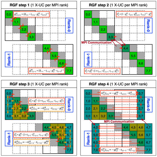
Figure 1.
The computational process of the recursive Green’s function (RGF) method. Computation is distributed with two message passing interface (MPI) processes and the workload belonging to a single MPI process is further parallelized with OpenMP threads. Step 3, which evaluates half of the off-diagonal sub-matrices of the inverse matrix, is the most time-consuming step, involving repeated multiplication of the sub-matrices of the original system matrix.
The size of sub-matrices and the number of sub-matrix multiplications increases as the size of the nanostructures to be simulated increases. We discuss the correlation between the size of a nanostructure and corresponding computing load with a square nanowire structure as shown in Figure 2a, where the transport happens along the X-direction. As shown in Figure 2b, the number of off-diagonal sub-matrices that need to be computed in step 3 increases in proportion to a square of the number of atomic unitcells that a nanostructure has along the X-direction (X-UC). The size of complex sub-matrices is related to the number of unitcells on the YZ-plane of a nanostructure (YZ-UC) and is proportional to (YZ-UC)2 as described in Figure 2c with a couple of examples. Here, the unitcell (UC) is defined as the smallest repeating unit in atomic crystals, and a single UC of cubic semiconductors has a total of 4 atomic layers along the [1 0 0] family of directions. Therefore, if X, Y, and Z are set to the [1 0 0], [0 1 0], and [0 0 1] directions, respectively, a system matrix describing a nanostructure having a single X-UC is composed of 4 × 4 sub-matrices, and the size of these sub-matrices is determined by the YZ-UC. Consequently, the computational burden of step 3 sharply increases as the size of a nanostructure increases.
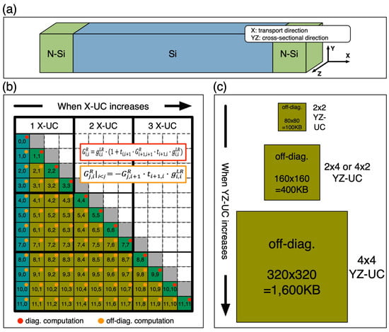
Figure 2.
The cost of the sub-matrix multiplication that must be paid according to the X-Y-Z size of the nanostructure to be simulated. (a) The nanowire structure that is subjected to quantum transport simulations consists of multiple atomic unitcells (UCs), and the transport happens along the X-direction. The computing cost sharply increases as the nanowire gets larger, so (b) the number of off-diagonal sub-matrices is proportional to (X-UC)2 and (c) the size of a sub-matrix increases in proportion to (YZ-UC)2, where X-UC and YZ-UC are the number of unitcells along the X-direction and on the YZ-plane of the nanowire, respectively.
2.2. Strategies for Performance Enhancement
This sub-section presents a detailed description of the four technical strategies that are employed to accelerate the RGF computation (particularly step 3 that involves a large number of sub-matrix multiplications) with the aid of manycore computing. We note that the multi-channel DRAM (MCDRAM), the high bandwidth memory on KNL processors (16 GB per node), has been utilized with the memkind library [18] only during the process of sub-matrix multiplication: if a sub-matrix multiplication needs to be conducted, the two source arrays are moved from DDR4 to MCDRAM. The result is then moved back to DDR4 and data in MCDRAM are deleted immediately after the multiplication is completed.
2.2.1. Data-Restructuring for SIMD and SIMT Operations
As mentioned in the Section 2.1, the core numerical operation of the RGF method is the multiplication of two sub-matrices. Even though a large number of sub-matrix multiplications are conducted in step 3, steps 1 and 4 also involve some multiplications. The first strategy we adopt to enhance the multiplication speed is data restructuring of complex sub-matrices. In many cases, a complex number (a single element of sub-matrices) is represented with a structure that has a real (r) and an imaginary number (i) as member variables as shown in Figure 3a. In this case, the matrix is constructed with the array of structures (AoS) [19], and r’s and the i’s of matrix elements are lined up next to each other in turn in the memory. If multiplication is conducted with AoS-type matrices as shown in the code snapshot given in Figure 3b, the access to matrix elements cannot be continuous in terms of memory address, but must happen with a stride of 2. Obviously, this type of data arrangement is not desirable for fetching multiple data due to the poor locality, and the single instruction multiple data (SIMD) or the single instruction multiple threads (SIMT) operations, which are the focal strength of manycore computing and are based the process of fetching multiple data, would lose their efficiency in handling multiplication.
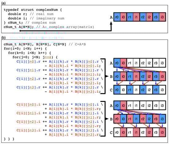
Figure 3.
Matrix multiplication with single instruction multiple data (SIMD) (or single instruction multiple threads (SIMT)) where two complex matrices are constructed with arrays of structures. (a) A real and an imaginary number are grouped into a structure to describe a single complex number, and arrays of structures are used to represent matrices. (b) During multiplication of two complex matrices, elements are accessed with a stride = 2, so the multiplication process cannot fully exploit the benefit of SIMD (or SIMT).
Consequently, we need to change the data structure of complex matrices to the structure of arrays (SoA) [19] as shown in Figure 4, since the original QAND code adopted an AoS-type data structure to construct matrices. In the SoA-type data structure, a single complex matrix can be represented with a structure that has two arrays, where one has real numbers and the other has imaginary numbers for matrix elements (it should be noted that if the size of each array is 1, the structure represents a complex number). In SoA-type complex matrices, r and i arrays are stored continuously in the memory as illustrated in Figure 4a. When multiplication of SoA-type complex matrices is conducted as the code snapshot in Figure 4b shows, the access to matrix elements can happen continuously in the memory, and therefore the performance of matrix multiplication can be enhanced with SIMD or SIMT operations using vector processing units (VPUs) in a KNL processor or GPU devices.

Figure 4.
Matrix multiplication with SIMD (or SIMT) where two complex matrices are constructed with structures of arrays. (a) Matrix elements are constructed with two arrays that store real and imaginary numbers. (b) During multiplication of two complex matrices, elements can be accessed continuously (stride = 1), so the benefit of SIMD (or SIMT) can be fully exploited and multiplication can be done more efficiently than the case discussed in Figure 3.
2.2.2. Blocked (Tiled) Matrix Multiplication
Utilization of blocked matrices or matrix blocking, which is the second strategy we adopt, is well known as one of the sound techniques for enhancing the performance of dense matrix multiplication, since it helps increase the cache hit ratio during the multiplication process [20]. The major question here is how to determine the block size with which target matrices subjected to multiplication are decomposed. For determination of the optimal block size, it is essential to consider the size of the cache memory available in computing resources where multiplication will be conducted. In KNL manycore processors, each CPU core has a 32 kB L1 cache and two CPU cores (a tile) sharing 1 MB L2 cache [12], and therefore the block size per physical core (equivalent to a single thread unless hyper-threading is enabled) must be smaller than 32 kB (32 × 1024 bytes). In a problem of A × B = C where A, B, and C are SoA-type complex matrices, the continuous data access occurs in the two matrices B and C (see the code snapshot in Figure 4b). In KNL systems, therefore, it is desirable to control the size of a single block-matrix so as not to exceed 16 kB. In GPU computing, the above-mentioned technique (“blocked matrix multiplication”) is commonly referred to as “tiled matrix multiplication” [21]. In computing systems with KNL processors or traditional multicore processors, we cannot but change the pattern of data access with estimation of the block size because data in the cache memory cannot be directly controlled. In the case of GPU devices, however, users can manage the shared memory that acts like the L1 cache in the host processors, so the data that need to be accessed quickly can be stored to the shared memory at users’ convenience.
In this study, the size of a single block (tile) matrix is set to 32 × 32 since a 32 × 32 block matrix stores 1024 complex numbers and therefore uses 16 kB memory (16 bytes for a single complex number that consists of two 8-byte double-precision numbers representing a real and an imaginary number). As addressed, the continuous data access happens in two block matrices in the multiplication process, so the block size of 32 × 32 would be suitable to a 32 kB cache memory that is the case of the L1 cache of a single KNL processor. In the case of GPU devices, users are able to set the size of the shared memory, and its maximum size depends on the device model. Although the NVIDIA Quadro GV100 devices that we use in this study allow users to increase the size of the shared memory up to 96 kB [21], here we set it to 32 kB to fully exploit the power of GPU resources. Then, a total of 1024 threads are generated per GPU device to let a single thread handle a single element of complex block matrices (1024 = 32 × 32). Further details of the resource occupancy of GPU devices will be covered in the Results and Discussion section.
2.2.3. Thread Scheduling for Execution of Nested Loops
As already addressed, all of the computing load of complex matrix multiplication in the RGF steps is parallelized with multiple threads. While the technique of blocked (tiled) matrix multiplication can help increase the cache hit ratio and improve data locality, a load imbalance among threads can happen depending on the size of sub-matrices and the number of employed threads, which would deteriorate the efficiency of thread-utilization. This issue is clearly described in Figure 5 with an exemplary condition whose details are summarized as below.
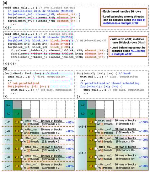
Figure 5.
Effects of blocked (tiled) matrix multiplication and thread scheduling that are described with a 2560 × 2560 sub-matrix. (a) With no blocked matrix multiplication, the entire 2560 rows are processed in parallel with 32 threads (per MPI process). If multiplication is performed in the unit of a 32 × 32 matrix, data locality improves but 80 (block) rows are processed with 32 threads so we have the issue of load imbalance. (b) This load imbalance (left) can be resolved by processing both j-loop and matrix multiplication (subroutine cMat_mul) in parallel (right), where we split total threads into two groups to process the j-loop in parallel, resolving the issue of load imbalance from cMat_mul. Note that here the simulated structure has 2 unitcells and 8 atomic layers along the X-direction since a single [100] unitcell has 4 atomic layers.
- The cubic semiconductor nanostructure has 2 unitcells along the X([1 0 0])-direction. The system matrix consists of 8 × 8 sub-matrices since a single [1 0 0] unitcell has 4 atomic layers.
- The nanostructure has 8 × 16 unitcells on the YZ([0 1 0] and [0 0 1])-plane. Since we use a 10-band tight-binding model and a single [1 0 0] unitcell has 2 atoms per atomic layer, the size of a sub-matrix becomes 2560 × 2560 (= 16 × 8 × 2 × 10).
- The block size is 32 × 32 and is equal to the L1 cache size of a KNL processor.
- The number of threads used in a single MPI process is 32, since a single KNL node we use has 64 physical cores and 2 MPI processes are employed for RGF computation.
- We focus on the moment of processing the 6th iteration of i-loop (i = 1 and j = 7→6→5→4→3→2).
When the multiplication process is conducted in parallel with no use of the blocked matrix multiplication technique (as shown in the upper side of Figure 5a), the entire 2560 rows of a sub-matrix are processed with 32 threads, and each thread then takes equal computing load processing 80 rows evenly. When the technique of blocked matrix multiplication is applied, however, the branch unit of the for-loop becomes the block size (= 32) rather than the element size (= 1), and the target of the matrix multiplication is changed to an 80 × 80 block matrix instead of a 2560 × 2560 matrix (as shown in the lower side of Figure 5a). Consequently, the problem becomes “to process 80 rows (of blocks) with 32 threads” and we have an issue of load imbalance since the quotient between the number of rows and threads is not an integer. In other words, the workload is not evenly distributed among 32 threads. In this case, more specifically, half of the 32 threads (group A) process 48 rows of blocks (3 rows per thread) and the other half takes 32 rows (2 rows per thread). So, to complete the task, 32 threads need to run 3 cycles but only 80 threads (= 32 × 2 + 16) are actually participating in the computation. The efficiency of thread utilization therefore becomes 80/96 = ∼83%. To resolve this issue and improve the efficiency of thread utilization, we revise a policy of thread scheduling with the following processes:
- Decompose j-loop by 2n iterations to determine the number of threads participating in the parallelization of each decomposed loop ().
- Adjust the number of threads participating in matrix multiplication (the subroutine cMat_mul) () in each decomposed loop. × should be always equal to the number of threads that belong to a single MPI process (32 in this case).
The following example presents a more detailed description of how the above-mentioned policy of thereat scheduling can help reduce the issue of load imbalance when the technique of blocked matrix multiplication is applied.
- Decompose the number of iterations of j-loop (6) into 4 and 2 (6 = 22 + 21) as shown in the right side of Figure 5b.
- The 4 iterations of j-loop (j = 7→6→5→4) are executed simultaneously with 4 threads, and cMat_mul is processed with 8 threads (32/4 = 8). In this case, all the 32 (4 × 8) threads execute matrix multiplication simultaneously, and the issue of load imbalance does not exist since 80 rows are processed in parallel with 8 threads.
- Once the above 4 iterations are completed, we reschedule threads such that the remaining 2 iterations (j = 3→2) are executed with 2 threads, and cMat_mul is processed with 16 threads (32/2 = 16). This case does not have the issue of load imbalance either since each of the 16 threads can process 5 rows.
When the proposed policy of thread scheduling is applied, the efficiency of thread utilization obviously becomes 100% on average for the exemplary case ((100 × 4 + 100 × 2)/6). Since the above-mentioned example only describes the case when i = 1, we calculated the efficiency at other iterations of i-loop and summarized the results in Table 1, which indicates that the efficiency of thread utilization becomes 96.01% on average in step 3 of RGF computation when the technique of thread scheduling is applied, and the efficiency has been improved by roughly 13% compared to the result obtained with no thread scheduling (83%). It should be noted that, with the proposed technique, a 100% efficiency can be always achieved if the number of iterations of j-loop is even. Even if the number of iterations of j-loop is odd, the efficiency generally increases from ∼83.33% (the lowest value) to ∼100% as the number of iterations of j-loop increases, or equivalently, the nanostructure becomes longer along the X-direction.

Table 1.
Efficiency of thread utilization obtained with the policy of thread scheduling proposed in this work.
2.2.4. Offload Computing with GPU Accelerators
In spite of their excellent hardware performance as computing resources, GPU accelerators must involve communications with host processors through the PCI-E channel, and this communication overhead sometimes serves as one of the bottlenecks for performance enhancement. In general, workload offloading to GPU devices is done with the following three steps:
- Transfer the data to be computed in GPU devices from the host memory to the device memory. Here, host CPU cores control GPU devices using streaming, so each host sends block matrices to a physical GPU device using their own GPU stream.
- Conduct computation in GPU devices. Computation can be conducted simultaneously in both host and GPU devices, but GPU-only computation would be more preferable in terms of the speed as the hardware performance of GPU devices becomes better.
- Transfer the results of the computation from the device memory back to the host memory.
Accordingly, if data transfer between host processors and GPU devices occurs more frequently than computation, the strength driven with GPU devices for acceleration of workloads would be reduced. As the last strategy for performance improvement of RGF computation, we design a scheme of offload computing that can exploit the strength of GPU devices by reducing data transfer as much as possible. As addressed in the Section 2.1, step 3 of the RGF method is the most time-consuming step, and we therefore offload it to GPU devices to drive huge acceleration of sub-matrix multiplication. Step 3 of the RGF computation can be categorized into two parts. One is the process of diagonal sub-matrices (backward sweep) and the other is the process of off-diagonal sub-matrices, as indicated with red and orange arrows, respectively, in the bottom-left sub-figure of Figure 1.
As illustrated in Figure 6, computation in step 3 is processed in the unit of (sub-matrix) columns, and the workload of a single column is executed in parallel with the aid of a large number of threads and blocks available in GPU devices (detailed conditions will be presented in Section 3.1). Computation of sub-matrices at a specific columns is conducted with several sub-matrices that are either calculated in the previous column or newly transferred from the host (three or four sub-matrices must be transferred per column). Data transfer from device to host only happens in the last column. Since the number of sub-matrices that must be transferred between the host and the devices is almost linearly proportional to X-UC, while the number of sub-matrices subjected to multiplication increases approximately with (X-UC)2 (Figure 2), the proposed scheme of offload computing would become more beneficial in terms of computing speed as the nanostructure becomes longer along the transport direction (X-direction). For example, when X-UC of the nanostructure is 2, each MPI process must handle three columns of sub-matrices (Figure 6) since the system matrix is decomposed with 2 MPI processes. In this case, per MPI process, the host must send 10 sub-matrices (4 + 3 + 3) to GPU devices, and each GPU device must send 4 sub-matrices to the host (a total of 14 sub-matrices). If X-UC increases to 100, the number of sub-matrices that must be transferred between the host and the GPU devices becomes 798 (host-to-device: 4 + 3 × 198, device-to-host: 200) per MPI process. However, the number of sub-matrices that involve the multiplication process per MPI process increases from 9 (X-UC = 2) to 20,999 (X-UC = 100), so it is obvious that the pure computational burden relative to the PCI-E communication burden in step 3 becomes much larger when X-UC = 100 than when X-UC = 2.
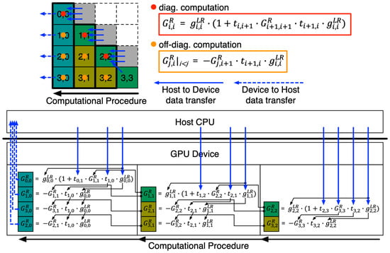
Figure 6.
The scheme of offload computing for RGF step 3 is described by the case when the nanostructure has a single unitcell along the X-direction (X-UC = 1). Half of the off-diagonal sub-matrices of the inverse matrix are evaluated with the consecutive multiplication of sub-matrices, whose computational flow is shown with large black arrows. Sub-matrices needed for computation at each column are either transferred from the host or derived from the calculation at the previous column. The performance gain derived with offload computing becomes larger as the nanostructure has more X-UCs, since the increase in the number of matrix multiplications is much bigger than the increase in the number of sub-matrices that must be transferred from the host.
3. Results and Discussion
3.1. Utilization Efficiency of GPU Devices for Offload Computing
NVIDIA provides the CUDA Occupancy Calculator [22] as a tool that enables developers to examine the efficiency of utilization of GPU resources for their own kernel codes. By providing the information of computing capability and using -Xptxas -v as options when compiling the GPU kernel code, we can check the detailed usage of GPU computing resources and, being fed by this information, the CUDA Occupancy Calculator returns the exact percentile value that shows how much GPU devices are well exploited. Since details of available computing resources vary depending on the GPU computing capability, it is critical to have a precise understanding of the architecture and the hardware specification of GPU devices that will be utilized to accelerate the kernel code. As addressed, 1024 threads are utilized to parallelize a single 32 × 32 complex block matrix. Since the NVIDIA Quadro GV100 device (computing capability 7.0) allows mapping of up to 2048 threads per streaming multiprocessor (SM), a total of two thread blocks are utilized per SM. Since a single block matrix requires 16 kB to store all of its complex elements and continuous memory access happens in two block matrices during the multiplication process, the size of the shared memory per single thread-block and the L1 cache per SM is set to 32 and 64 kB, respectively, and, with this condition, we observe that 100% occupancy of GPU devices can be achieved.
3.2. Performance of End-To-End Simulations
The performance of end-to-end simulations was investigated with rigorous tests that were conducted with a focus on (1) the speed in a single computing node and (2) the strong scalability in large-scale computing environment. The main purpose of the single-node performance tests was to understand and verify the efficiency of the optimization strategies (discussed in the Section 2.2) for acceleration of RGF computational processes (Figure 1). Therefore, simulations were conducted for a single energy point and in the NINJA developer platform (KNL, Xeon Phi 7210) equipped with two NVIDIA Quadro GV100 GPU devices. Since typical simulations of quantum transport include more than hundreds of energy points, the multi-node tests aim to explore the scalability of realistic simulations in supercomputers, where the MPI processes are grouped into two levels such as high-level and low-level and are used to parallelize energy points and RGF computation, respectively. The scalability tests were conducted with simulations of 2048 energy points in the NURION supercomputer [14], which has a total of 8305 KNL (Xeon Phi 7250) nodes and was ranked 21st in the TOP500 site as of November 2020. The target structure of simulations was a silicon nanowire, where the transport (X-) direction was [100] and the channel was grown along the [001] direction. X-UC and YZ-UC of the nanowire were 100 and 8 × 16, respectively. Since a single [100] unitcell of cubic semiconductors has 8 atoms, the nanowire structure has a total of 102,400 atoms (= 100 × 8 × 16 × 8), and the size of the system matrix becomes 1,024,000 × 1,024,000, since a set of 10 localized bases is employed to describe a single silicon atom.
Table 2 shows the details of the computing environment where single-node performance tests were conducted. For precise examination of the effects driven by the optimization strategies discussed in Section 2.2, single-node performance tests were conducted in the five cases as shown in Table 3, where strategies were applied selectively in each test case (MPI and OpenMP parallelization and utilization of MCDRAM were applied in default). Table 4 shows the details of the computing environment where the multi-node tests were conducted. In this case, unlike the case for the single-node tests, a single MPI process was used per computing node so two nodes were in charge of RGF computation for a single energy point. All the optimization techniques except offload computing were used for the multi-node tests since the NURION supercomputer does not support GPU devices. In addition, MCDRAM was used as a last-level (L3) cache memory (cache mode) as the memkind library is not supported.
Table 2.
Computing environment for single-node performance tests.
Table 3.
Cases of single-node performance tests and techniques used in each case.
Table 4.
Computing environment for multi-node scalability tests.
Figure 7 shows the results of the single-node performance tests. With only MPI and OpenMP parallelization and MCDRAM utilization (Case 1), the end-to-end simulation per energy point took slightly longer than 21 h, and we observe that almost 95% of the total wall-time (∼20 h) was occupied by step 3. When the data restructuring (AoS→SoA) was applied to the system matrix (Case 2), the overall performance of the RGF computation improved by a factor of ∼1.56 compared to the result for Case 1, and this was clearly due to acceleration of the sub-matrix multiplication, which supports that the AVX-512 SIMD operation, one of the unique features of KNL processors, works more efficiently with SoA-type than AoS-type data structures. By applying the technique of blocked matrix multiplication (Case 3), we were able to drive additional performance improvements, where the simulation became faster by factors of 2.72 and 1.75 with respect to the results for Cases 1 and 2, respectively. Again, the major contribution of speed-up here can be found from step 3, and it can be concluded that the performance of RGF computation is remarkably affected by the locality of sub-matrix elements.

Figure 7.
Results of single-node performance tests. The wall-time of the entire RGF process is split into the 4 components that indicate the time taken to complete the 4 steps described in Figure 1. In the five test cases, the computation was conducted with one or more performance optimization enhancement techniques, according to the plan summarized in Table 3. Compared to the unoptimized case (Case 1 in Table 3), the performance of the entire computation and step 3 were improved by factors of 19.35 and 48.57, respectively, when all four optimization techniques were used.
We also observed that the technique of thread-scheduling is helpful for accelerating RGF computation. With this technique (Case 4), the wall-time of the overall computation was reduced by factors of 3.14 and 1.15 (3.27 and 1.17 for step 3) compared to the results of Cases 1 and 3, respectively. It must be noted that a 17% reduction of the wall-time of step 3, which was solely driven with thread scheduling, is closely related to the improved efficiency of thread utilization. In Section 2.2, we explained how scheduling can help increase efficiency (83.3% → 96%) with an exemplary nanostructure that has an X-UC of 2. In the case of our target structure (a silicon nanowire that has a total of 100 unitcells along the X-direction), the utilization efficiency reached 99.7% with the scheduling technique, showing a 16.4% improvement with respect to the result obtained with no thread scheduling (83.3%). Finally, in Case 5 where the computational load of step 3 was offloaded to GPU devices as described in Section 2.2 and Figure 6, the largest performance gain was obtained and the total execution time was reduced by a factor of 6.17 compared to Case 4, which is the best result obtainable with a single KNL node. The acceleration driven with GPU computing was more remarkable in step 3, whose wall-time turned out to be reduced by a factor of 14.83 compared to Case 4. The results of the single-node performance tests clearly demonstrate that all four performance optimization techniques (data restructuring, blocked matrix multiplication, thread scheduling, and offload computing) contributed significantly to enhancing the speed of RGF simulations (particularly step 3). Overall, when all four techniques are used, the entire computation can be completed in about 1 h. With no optimization techniques (Case 1), step 3 took almost 95% of the total wall-time. However, in Case 5, where all the techniques were used, this ratio dropped to ∼37.5% and the most time-consuming part was step 1 (∼47% of the total wall-time).
Figure 8a shows the results of the scalability test for the RGF calculation that was conducted with 2048 energy points in 512–2048 computing nodes of the NURION supercomputer. The time needed to complete end-to-end simulation was measured as ∼30.30 h when 512 computing nodes were used, and the time dropped to ∼15.20 and ∼7.63 h when 1024 and 2048 nodes were employed, respectively. Since the time taken for MPI communication, which only happens between every two nodes (in steps 2 and 4 of the RGF computation—see Figure 1) that are in charge of the computation for a single energy point, was smaller than 1000 s for all the three cases, the scalability was good and showed a ∼99% parallel efficiency on average as a ∼3.97× speed-up was achieved with 4x increased computing nodes (512 → 2048). The transmission coefficient (TR) and local density of states (LDOS), which were obtained as a function of energy from the simulation, are shown in Figure 8b,c, respectively. Representing the energy-dependent ballistic quantum conductance and electron density, the TR and LDOS profile were utilized to calculate the current and charge distribution in the nanowire, and were nonzero only at the energy range above the conduction band minimum of the nanowire (∼1.16 eV) where the path of electron conduction exists. Note that the results of the scalability tests here clearly indicate that simulations of large-scale atomic structures involving a large number of energy points, which are critical for a precise modeling of quantum transport behaviors of realistically sized nanoscale devices, can be completed in several hours with the aid of supercomputers.
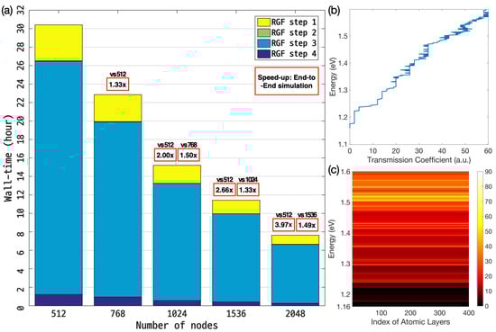
Figure 8.
(a) Results of multi-node scalability tests. A silicon nanowire consisting of 102,400 atoms was simulated with 2048 energy points in 512–2048 computing nodes of the NURION supercomputer. Since the MPI communication happens only between two nodes that are in charge of RGF computation for a single energy point, the communication time turned out to be less than 1000 s for all the three cases, and thus the scalability was good, supporting the supercomputer-driven feasibility of handling quantum transport simulations that normally involve more than several hundreds of energy points. (b) The transmission coefficient and (c) local density of states that are obtained with simulations show ballistic conductance and channel electron density as a function of energy.
4. Conclusions
In this study we proposed and discussed technical strategies to accelerate quantum transport simulations with manycore computing. The four optimization techniques, which are data restructuring, matrix tiling, thread scheduling, and offload computing, were applied in our in-house code package that employs the recursive Green’s function (RGF) as a backbone algorithm and uses atomistic tight-binding models to describe electronic structures of nanoscale devices. The effects of the optimization techniques on end-to-end simulations were elaborately examined through rigorous tests in the computing resources of Intel Xeon Phi Knights Landing (KNL) processors and NVIDIA general-purpose graphics processing unit devices. By applying the four techniques, we observed that the wall-time of the entire RGF computational processes could be reduced by up to a factor of 19.3× compared to the unoptimized case, which was due to the dramatic acceleration (up to 48.6×) of the core numerical step where multiplication of dense complex matrices is repeatedly conducted in a recursive manner. End-to-end simulations involving a large number of energy points, which are essential for a precise prediction of transport characteristics, were also conducted in a world-class supercomputer, and good scalability was observed up to 2048 KNL nodes. Even though we focused on a specific algorithm, the details of the optimization techniques that this work has delivered are universal and practical since they are used for the multiplication of dense complex matrices, which is one of the most basic operations that is frequently used in a large variety of numerical problems.
Author Contributions
Conceptualization, H.R.; methodology, Y.J. and H.R.; formal analysis, Y.J. and H.R.; investigation, Y.J. and H.R.; writing—original draft preparation, Y.J. and H.R.; writing—review and editing, Y.J. and H.R.; supervision, H.R. All authors have read and agreed to the published version of the manuscript.
Funding
This work was carried out as the Intel Parallel Computing Center (IPCC) project supported by the Intel Corporation, USA, and was also supported by the grant from the National Research Foundation of Korea (NRF-2020M3H6A1084853) funded by the Korean government (MSIP).
Data Availability Statement
The datasets generated during and/or analyzed during the current study are available from the corresponding author on reasonable request.
Acknowledgments
The NURION high-performance computing resource was extensively utilized for performance tests of large-scale simulations.
Conflicts of Interest
The authors declare no conflict of interest.
References
- Datta, S. Nanoscale device modeling: The Green’s function method. Superlattices Microstruct. 2000, 28, 253–278. [Google Scholar] [CrossRef]
- Abadi, R.M.I.; Saremi, M. A Resonant Tunneling Nanowire Field Effect Transistor with Physical Contractions: A Negative Differential Resistance Device for Low Power Very Large Scale Integration Applications. J. Electron. Mater. 2018, 47, 1091–1098. [Google Scholar] [CrossRef]
- Naser, M.A.; Deen, M.J.; Thompson, D.A. Photocurrent Modeling and Detectivity Optimization in a Resonant-Tunneling Quantum-Dot Infrared Photodetector. IEEE Trans. Quantum Electron. 2010, 46, 849–859. [Google Scholar] [CrossRef]
- Quhe, R.; Li, Q.; Zhang, Q.; Wang, Y.; Zhang, H.; Li, J.; Zhang, X.; Chen, D.; Liu, K.; Ye, Y.; et al. Simulations of Quantum Transport in Sub-5-nm Monolayer Phosphorene Transistors. Phys. Rev. Appl. 2018, 10, 024022. [Google Scholar] [CrossRef]
- Jancu, J.M.; Scholz, R.; Beltram, F.; Bassani, F. Empirical spds* tight-binding calculation for cubic semiconductors: General method and material parameters. Phys. Rev. B 1998, 57, 6493. [Google Scholar] [CrossRef]
- Cauley, S.; Jain, J.; Koh, C.K.; Balakrishnan, V. A scalable distributed method for quantum-scale device simulation. J. Appl. Phys. 2007, 101, 123715. [Google Scholar] [CrossRef]
- Ryu, H.; Jeong, Y.; Kang, J.H.; Cho, K.N. Time-efficient simulations of tight-binding electronic structures with Intel Xeon Phi™ many-core processors. Comput. Phys. Commun. 2016, 209, 79–87. [Google Scholar] [CrossRef]
- Ryu, H.; Kwon, O.K. Fast, energy-efficient electronic structure simulations for multi-million atomic systems with GPU devices. J. Comput. Electron. 2018, 17, 698–706. [Google Scholar] [CrossRef]
- Vogl, P.; Hjalmarson, H.P.; Dow, J.D. A Semi-empirical tight-binding theory of the electronic structure of semiconductors. J. Phys. Chem. Solids 1983, 44, 365–378. [Google Scholar] [CrossRef]
- Ryu, H.; Hong, S.; Kim, H.S.; Hong, K.H. Role of Quantum Confinement in 10 nm Scale Perovskite Optoelectronics. J. Phys. Chem. Lett. 2019, 10, 2745–2752. [Google Scholar] [CrossRef] [PubMed]
- Ryu, H.; Kim, J.; Hong, K.H. Atomistic study on dopant-distributions in realistically sized, highly p-doped si nanowires. Nano Lett. 2015, 15, 450–456. [Google Scholar] [CrossRef] [PubMed]
- Sodani, A. Knights landing (KNL): 2nd generation Intel® Xeon Phi processor. In Proceedings of the 2015 IEEE Hot Chips 27 Symposium (HCS), Cupertino, CA, USA, 22–25 August 2015; pp. 1–24. [Google Scholar] [CrossRef]
- NVIDIA Quadro GV100 GPU Device. Available online: https://www.nvidia.com/content/dam/en-zz/Solutions/design-visualization/productspage/quadro/quadro-desktop/quadro-volta-gv100-data-sheet-us-nvidia-704619-r3-web.pdf (accessed on 21 January 2021).
- The NURION Supercomputer. Available online: https://www.top500.org/system/179421/ (accessed on 21 January 2021).
- Walker, D.; Dongarra, J. MPI: A standard message passing interface. Supercomputer 1996, 12, 56–68. [Google Scholar]
- Dagum, L.; Menon, R. OpenMP: An industry standard API for shared-memory programming. IEEE Comput. Sci. Eng. 1998, 5, 46–55. [Google Scholar] [CrossRef]
- Kirk, D. NVIDIA CUDA software and GPU parallel computing architecture. In Proceedings of the 6th International Symposium on Memory Management (ISMM), Montreal, QC, Canada, 21–22 October 2007; pp. 103–104. [Google Scholar] [CrossRef]
- Cantalupo, C.; Venkatesan, V.; Hammond, J.; Czurlyo, K.; Hammond, S.D. Memkind: An Extensible Heap Memory Manager for Heterogeneous Memory Platforms and Mixed Memory Policies; Technical Report; Sandia National Laboratories: Albuquerque, NM, USA, 2015. [Google Scholar]
- Strzodka, R. Abstraction for AoS and SoA layout in C++. In GPU Computing Gems Jade Edition; Elsevier: Amsterdam, The Netherlands, 2012; Volume 31, pp. 429–441. [Google Scholar]
- Lam, M.D.; Rothberg, E.E.; Wolf, M.E. The cache performance and optimizations of blocked algorithms. ACM SIGOPS Oper. Syst. Rev. 1991, 25, 63–74. [Google Scholar] [CrossRef]
- Park, N.; Hong, B.; Prasanna, V.K. Tiling, block data layout, and memory hierarchy performance. IEEE Trans. Parallel Distrib. Syst. 2003, 14, 640–654. [Google Scholar] [CrossRef]
- CUDA Occupancy Calculator. Available online: https://docs.nvidia.com/cuda/cuda-occupancy-calculator/index.html (accessed on 21 January 2021).


Publisher’s Note: MDPI stays neutral with regard to jurisdictional claims in published maps and institutional affiliations. |
© 2021 by the authors. Licensee MDPI, Basel, Switzerland. This article is an open access article distributed under the terms and conditions of the Creative Commons Attribution (CC BY) license (http://creativecommons.org/licenses/by/4.0/).