Article

Predictive Fixed Switching Maximum Power Point Tracking Algorithm with Dual Adaptive Step-Size for PV Systems

1
Institute for Electrical Drive Systems and Power Electronics (EAL), Technical University of Munich (TUM), 80333 Munich, Germany
2
Electrical Engineering Department, Faculty of Engineering, Assiut University, Assiut 71516, Egypt
3
Electrical Engineering Department, Faculty of Engineering, Menoufia University, Shebin El-Koum 32511, Egypt
*
Author to whom correspondence should be addressed.
Electronics 2021, 10(24), 3109; https://doi.org/10.3390/electronics10243109
Submission received: 17 November 2021 / Revised: 6 December 2021 / Accepted: 10 December 2021 / Published: 14 December 2021

Abstract

:
Maximum power point tracking (MPPT) is an essential and primary objective in photovoltaic (PV) systems implementation. Thus, in this article, the predictive fixed switching MPPT technique is proposed for a two-stage PV system, where the system under consideration consists of a PV source, boost converter, and two-level inverter. The MPPT design is based on dual adaptive step-size realization to limit the duty cycle oscillations at a steady state. Furthermore, the PI controller is eliminated, which simplifies the MPPT implementation. The suggested tuning procedure of the duty cycle is compared with the conventional adaptive step-size perturb and observe (P&O) method. The inverter is controlled using an efficient finite-set model predictive control (FS-MPC) algorithm with reduced computation burden, where the optimal switching state vector is identified based on the polarity of the reference voltage in the α - β reference frame and without any need for sector determination. Furthermore, the cost function of the FS-MPC algorithm is modified to include the reduction of the switching frequency as a secondary objective for the inverter control. The overall control methodology is evaluated using experimental results at different operating conditions.

1. Introduction

Photovoltaic (PV) source has nonlinear characteristics [1], where the power-voltage (P-V) curve exhibits one peak at uniform radiation conditions [2]. This, in turn, necessitates the evolution of a maximum power point tracker (MPPT) technique [3]. In such techniques, the maximum power point (MPP) of the P-V curve is chased [4]. Different methods have been implemented in the literature [5,6,7] for that purpose. However, they can be mainly classified into model-based algorithms, training-based methods, and searching procedures. The model-based methods depend on a mathematical model for representing the characteristics of the PV source and finding an exact or accurate formulation of the MPP. The training-based approaches employ artificial neural network or fuzzy logic controller, which need prior training information to perform the MPPT function. In the searching techniques, the measured voltage and/or current of the PV source are utilized to direct the control parameter to the MPP, and within this category lie the well-known perturb and observe (P&O) and incremental conductance (INC) methods [8].
Generally, the PV systems can be categorized into single-stage and two-stage systems. However, the most popular configuration is the two-stage system, where the MPPT operation is managed in the first stage (DC-DC) [9]. Furthermore, the active and reactive power exchange with the grid is realized in the second stage (DC-AC). In this regard, and for grid integration, different strategies have been implemented to regulate the active and reactive power. Popularly, the voltage-oriented control (VOC) and direct power control (DPC) are implemented for this purpose [10]. The VOC uses the cascaded loop structure of the voltage loop, and the current loop to obtain the reference voltage (using PI controllers), which is fed to the modulation stage for generation of the switching actions. Obviously, the switching frequency of this method is fixed, whereas the DPC utilizes a hysteresis controller to generate the switching states for the converter knowing the grid–voltage position (via look-up table procedure). Therefore, the switching behavior of this method is variable. However, the implementation is very simple without any tuning efforts. Recently, model predictive control has gotten a significant attention, especially the finite-set model predictive control (FS-MPC), in which the optimal switching state of the converter is applied directly according to a predefined cost function [11].
The main classification of model predictive control techniques are continuous-set model predictive control, finite-set model predictive control, and dead-beat predictive control [9,10]. Numerous efforts have been made to employ model predictive control for MPPT implementation. In [12], FS-MPC with two-step prediction horizon is utilized for a boost converter, where the INC method is used to generate the reference current for the FS-MPC loop. A similar approach is developed in [13] for a flyback converter. However, additional sensors are required in these methods due to the prediction stage of the FS-MPC. In this respect, some attempts have been performed to reduce the number of utilized sensors. For example, sensor reduction is accomplished based on the model predictive control principle in [14]. Furthermore, a simple load observer is executed to account for potential variations in the load. A reduction based on the mathematical model of a multilevel boost converter is done in [15]. Nevertheless, still the dependency on the utilized converter is the major drawback of these methods, where the model parameter uncertainties may ruin the behavior of the MPPT. Predictive fixed switching frequency for Z-source inverter is proposed in [16]. However, the adaptive step-size design is model dependent in this approach. Furthermore, a PI controller is employed to obtain the duty cycle command, which increases the tuning efforts. A very similar technique is implemented for the boost converter in [17] and for LLC resonant converter in [18].
Bio-inspired methods are also addressed in the literature, especially for partial shading conditions, where the P-V curve has several peaks. However, the implementation of these algorithms is time consuming and complex, making it unsuitable for industry application [19]. Conventionally, P&O is the most popular approach for extracting the maximum power from the PV source. However, this method has a poor steady-state performance due to the oscillations inherited from its perturbation nature [20]. Therefore, adaptive step-size can be utilized to limit this oscillation, where a large step is used when the operating point is far from the MPP and a lower one is employed as the operating point approaches the MPP [21]. Furthermore, it has poor behavior under fast atmospheric conditions [22].
Considering the above, a new predictive fixed switching MPPT algorithm is proposed in this paper. The suggested technique uses only two sensors for maximum power extraction such as the case of the conventional MPPT techniques. Thus, it is suitable also for low-power PV applications. For the first time, and to the best of authors’ knowledge, two adaptive step-size are utilized in our scheme. The objective of the two-step design is minimizing the oscillations which happen at steady state of the duty cycle waveform. The proposed MPPT is compared with the conventional but adaptive step-size implementation of the P&O method. Further on, a multiobjective control for the inverter stage is achieved based on the FS-MPC, where current control is considered the main control objective. The secondary control objective is introduced as reduction of the switching frequency—thanks to the FS-MPC and the cost function, where several control purposes can be achieved within one control law. The weighting factor in the cost function is tuned based on the THD of the injected currents, i.e., the selection procedure of the weighting factor has an approximately negligible impact on the THD of the currents (the primary control objective). Therefore, the main contribution of the current study can be summarized as:
  • Predictive fixed switching MPPT technique implementation with only two sensors and without need for PI controller, which simplifies the overall control scheme.
  • Dual adaptive step-size design of the duty cycle command to reduce the oscillation at steady state.
  • Multiobjective control for the inversion stage, which are current control and switching frequency minimization.
  • Experimental verification of the proposed MPPT and inverter control at different operating conditions.
The rest of this paper is organized as follows: Section 2 presents the mathematical model of the two-stage PV system. The proposed MPPT and multiobjective inverter control are investigated in Section 3. The experimental evaluation and comparison are given in Section 4. The future work is addressed in Section 5. Finally, the outcome of the paper is concluded in Section 6.

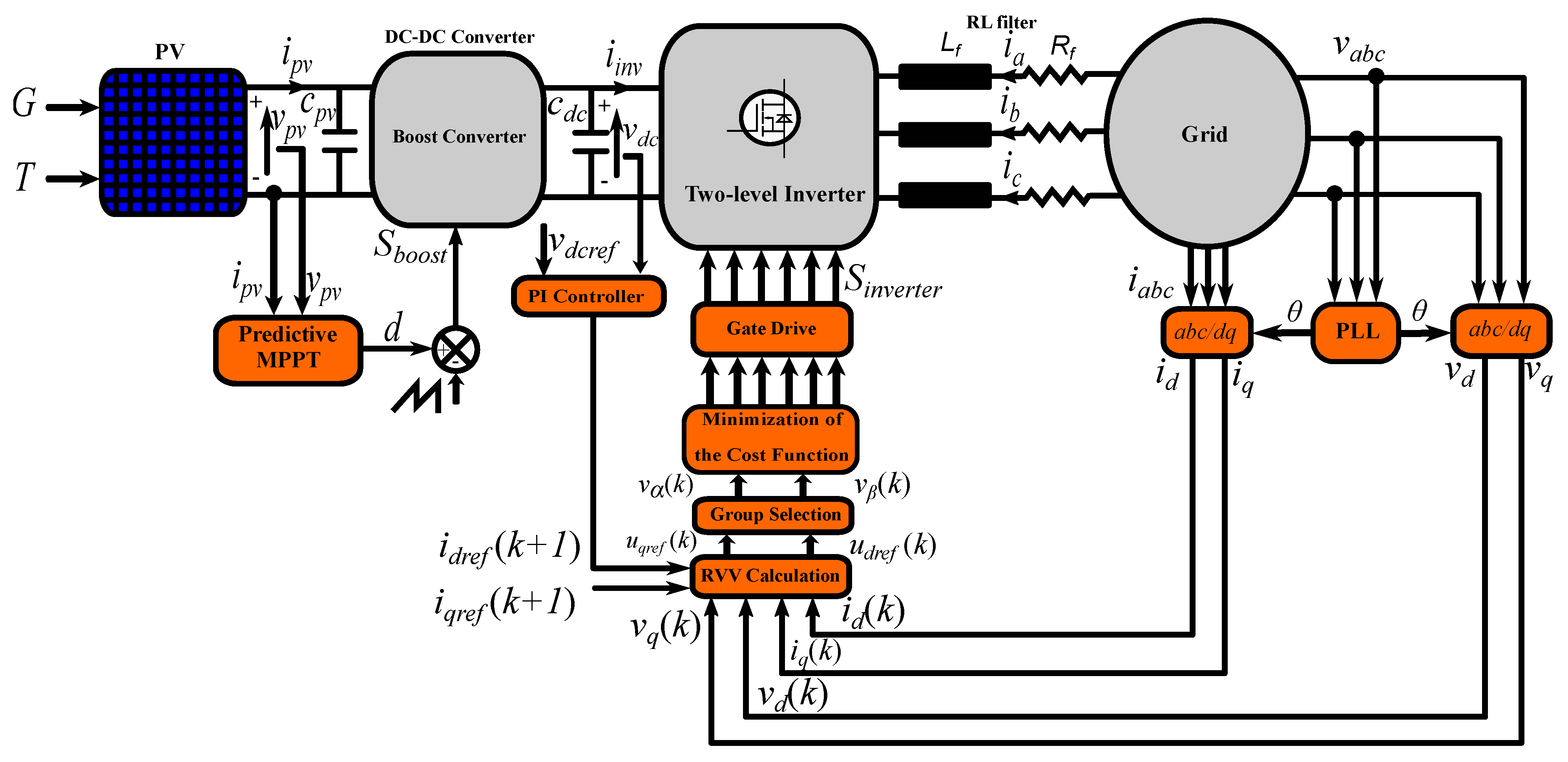
2. Model of the Two-Stage PV System

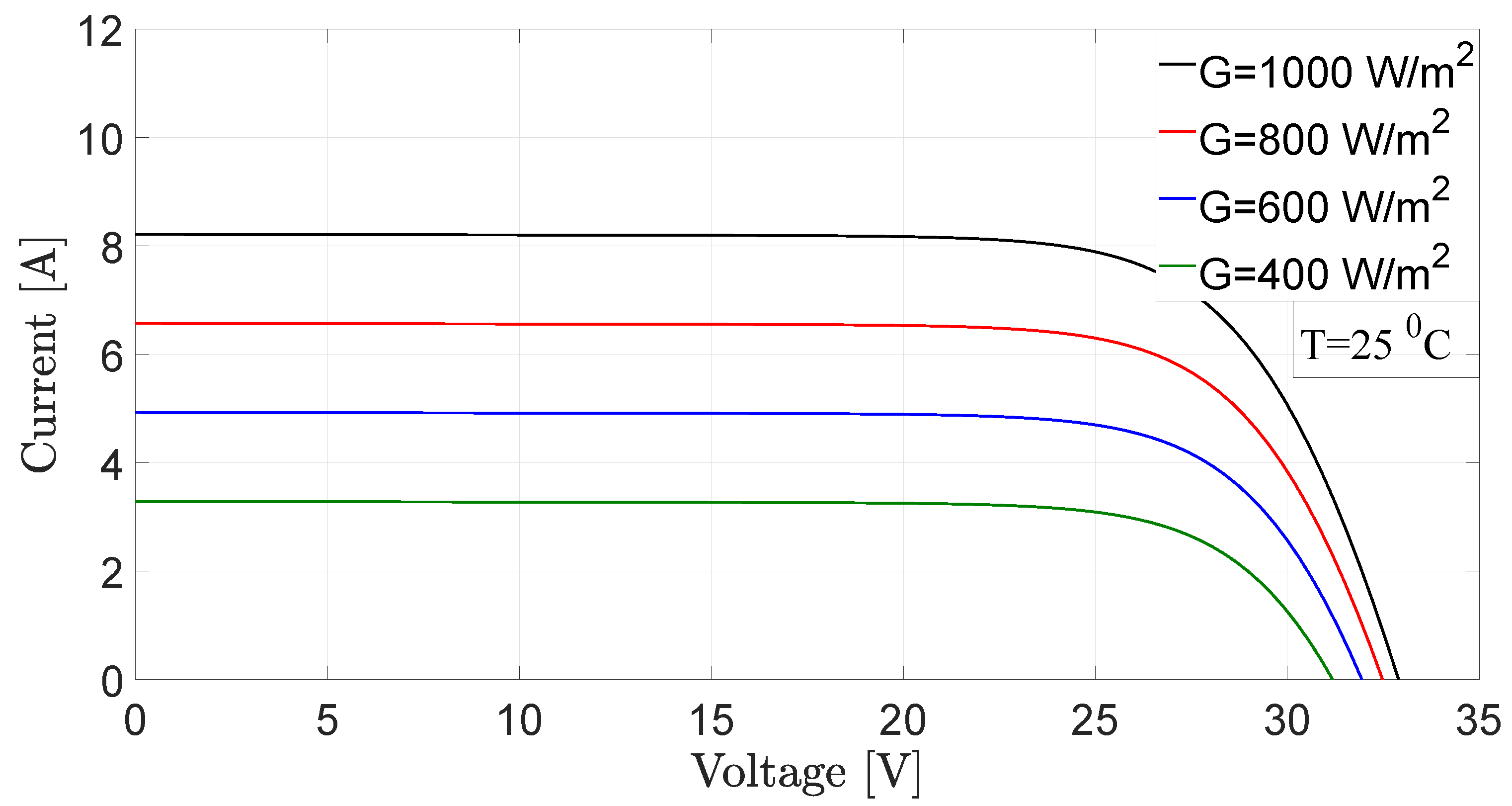
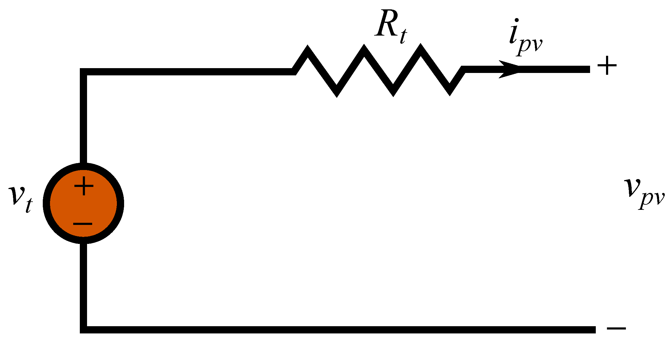
2.1. PV Source Modeling

The characteristics of the PV source can be represented using different models. However, the most popular model is the single-exponential one, due to its simplicity and accuracy [23]. According to that model, the current–voltage (I–V) relation can be described as [24,25]
i p v = i p h i o [ e ( v p v + i p v R s n N s v t ) 1 ] v p v + i p v R s R s h ,
where i p h is the photovoltaic current, i o is the diode saturation current, n is the diode ideality factor, R s is the module series resistance, R s h is the module shunt resistance, N s is the number of cells in one module, i p v is the terminal current, and v p v is the output voltage. Furthermore, the characteristics of the PV source at different atmospheric conditions are given in Figure 1 and Figure 2 [10].

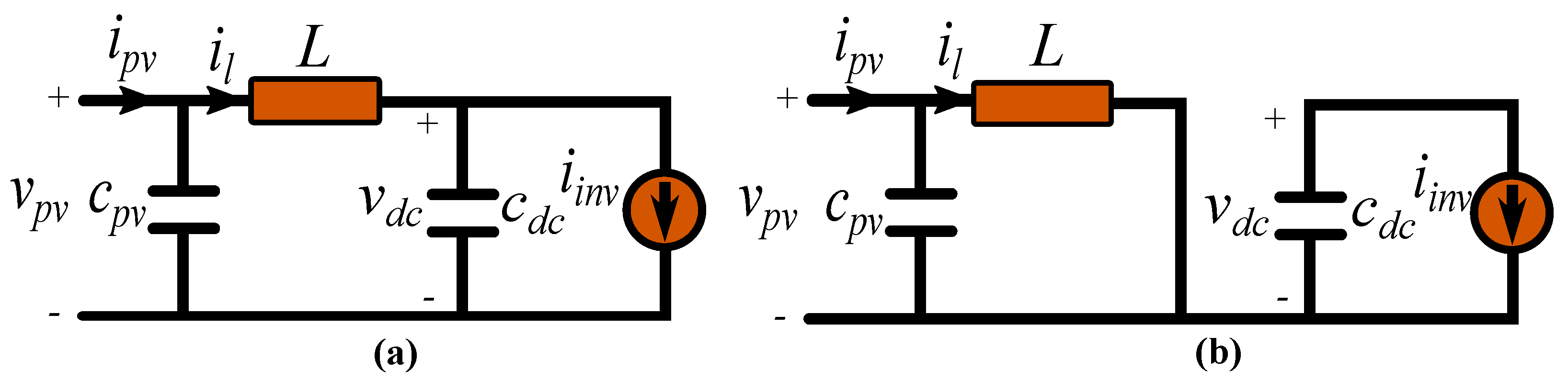
2.2. Boost Converter Model

The first stage of the PV system is the DC-DC converter (boost converter), where the MPPT function is executed. Moreover, it boosts the voltage of the PV source to enable grid integration. The model of the boost converter is specified by the actions of its switch. Thus, the modes of the boost converter are clarified in Figure 3. Simply put, the state-space behavior of the boost is characterized by [11].
x ˙ = A x + B u , y = C x + D u ,
where x = [ i p v v d c ] T is the state vector, u = [ v p v i i n v ] is the input vector, and y = v d c is the output. Furthermore, A , B , C , and D are the system matrices and are expressed as follows:
A = 0 1 d L 1 d c d c 0 , B = 1 L 0 0 1 c d c , C = 0 1 , D = 0 ,
where v d c is the DC-link voltage, i i n v is output current of the boost converter (input for the inverter), L is the boost inductance, c p v and c d c are the coupling capacitors at the PV and inverter side, respectively, and d is the duty cycle of the boost converter.

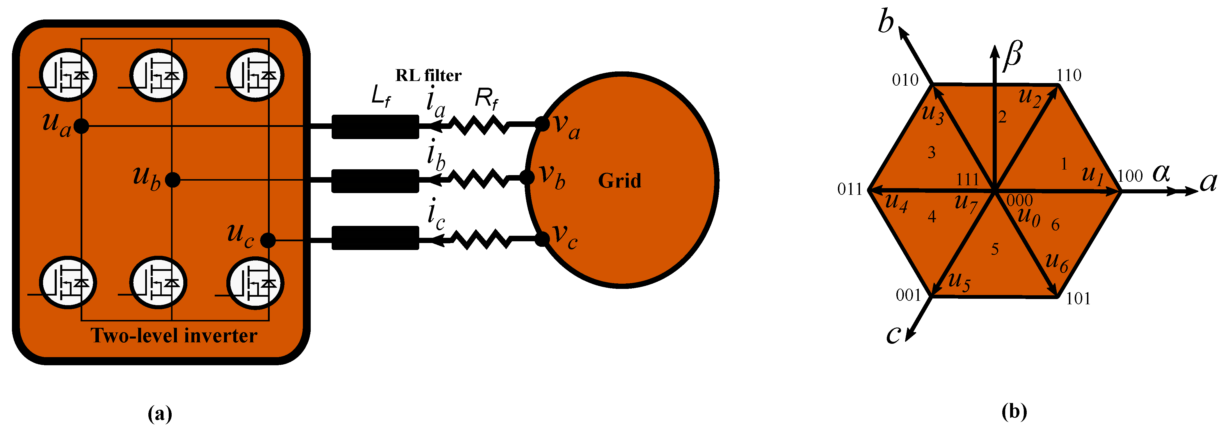
2.3. Model of the Two-Level Inverter with Grid Connection

Figure 4 shows the configuration of the grid-connected inverter. In fact, the two-level inverter has eight possible switching vectors, shown also in Figure 4 with the sector distribution (1–6). Table 1 briefly summarizes the potential switching actions and output voltages of the two-level inverter [9].
With respect to Figure 4 and applying KVL at the inverter output, the following results
v a b c = u a b c + L f d i a b c d t + R f i a b c ,
where v a b c are the grid voltages, u a b c are the inverter output voltages, i a b c are the line currents, L f is the filter inductance, and R f is the filter resistance.
In the stationary reference frame ( α - β ), Equation (4) can be rewritten as
v α β = u α β + L f d i α β d t + R f i α β .
Furthermore, and in the rotating reference frame (d-q), the same equation is expressed as
v d = u d + L f d i d d t + R f i d ω L f i q , v q = u q + L f d i q d t + R f i q + ω L f i d ,
where ω is the angular grid-frequency. As a result, the active and reactive power are expressed as
P = 3 2 ( v α i α + v β i β ) , Q = 3 2 ( v β i α v α i β ) ,
P = 3 2 ( v d i d + v q i q ) , Q = 3 2 ( v q i d v d i q ) .

3. The Proposed Control Strategy for the Two-Stage PV System

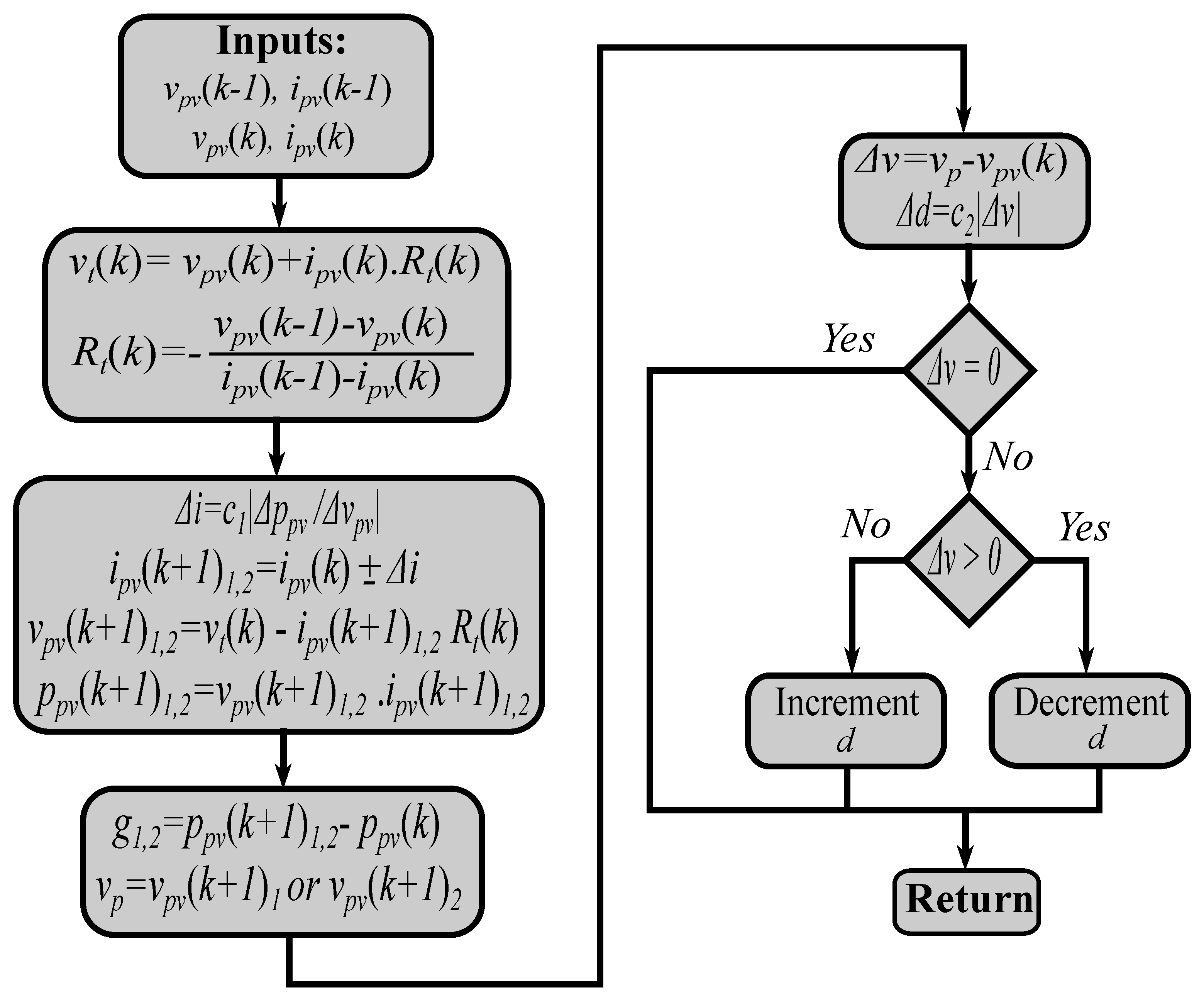
3.1. Predictive Fixed Switching MPPT with Dual Adaptive Step-Size Design

The predictive fixed switching method relies on the equivalent circuit of the PV source. Figure 5 shows the simplified model of the PV generator, in which the behavior of the PV circuit can be simplified to a voltage source connected to an equivalent resistance. Therefore, the design procedure of the suggested MPPT method can be summarized according to the following steps:
1. The predicted PV currents are computed as
i p v ( k + 1 ) 1 , 2 = i p v ( k ) ± Δ i ,
where i p v ( k + 1 ) is the PV current at next sampling instant, i p v ( k ) is the PV current at the present sampling instant, and Δ i is the step-size of the current. This step is adaptively tuned based on the gradient of the PV power with respect to the PV voltage as
Δ i = c 1 Δ p p v Δ v p v ,
where c 1 is a factor to be tuned.
2. Consequently, the predicted voltages are evaluated from
v p v ( k + 1 ) 1 , 2 = v t ( k ) i p v ( k + 1 ) 1 , 2 R t ( k ) ,
where v t ( k ) and R t ( k ) are the equivalent voltage and resistance of the PV source, respectively.
3. The equivalent voltage and resistance of the PV source are calculated as
v t ( k ) = v p v ( k ) + i p v ( k ) R t ( k ) ,
R t ( k ) = v p v ( k 1 ) v p v ( k ) i p v ( k 1 ) i p v ( k ) ,
where v p v ( k 1 ) and i p v ( k 1 ) are the PV voltage and current at the previous sampling instant.
4. The cost function for evaluation and selection is based on the predicted PV power, which can be expressed as
p p v ( k + 1 ) 1 , 2 = v p v ( k + 1 ) 1 , 2 i p v ( k + 1 ) 1 , 2 .
The predicted power is compared with the present PV power. Therefore, the cost function is finalized as
g 1 , 2 = p p v ( k + 1 ) 1 , 2 p p v ( k ) .
According to the cost function, the PV voltage corresponding to the higher power (between p p v ( k + 1 ) 1 and p p v ( k + 1 ) 2 ) is selected. Conventionally, this voltage is compared with the actual one, and the duty cycle is obtained using a PI controller. However, in our scheme, a second adaptive step is employed to minimize the difference between the optimal voltage and the actual value. This step is adjusted from
Δ d = c 2 | Δ v | ,
where c 2 is an adjustable factor and Δ v is the difference between the optimal voltage and the actual value.
Figure 6 shows the flow process of the proposed predictive fixed switching MPPT with two adaptive step-size design, where the equivalent voltage and resistance of the PV source are calculated. Then, the predicted currents are computed using the first adaptive step and based on the equivalent values of the source. Following, the predicted voltages are obtained, which enable the power computation and the cost function evaluation. According to the cost function, the optimal voltage is selected. Finally, the duty cycle command is obtained using the second adaptive step according to the distance between the actual and the optimal voltage.

3.2. Multiobjective FS-MPC with Reduced Computation Burden for Grid Integration

The conventional FS-MPC depends on the discrete nature of the system [26]. For the two level inverter, and as mentioned previously, the cost function is calculated eight times for the eight voltage vectors. The best voltage vector is selected among the eight vectors based on the design of the cost function. In brief, the design of the conventional FS-MPC for the two-level inverter can be summarized as follows:
Firstly, the predicted currents are calculated from the following, which is the discrete form of Equation (6):
i d ( k + 1 ) = ( 1 T s R f L f ) i d ( k ) + ω T s i q + T s L f ( v d ( k ) u d ( k ) ) , i q ( k + 1 ) = ( 1 T s R f L f ) i q ( k ) ω T s i d + T s L f ( v q ( k ) u q ( k ) ) .
Secondly, the optimal voltage vector is applied to the inverter based on the cost function design as
g i = | i d ( k + 1 ) u 0 , . . , 7 i d r e f ( k + 1 ) | + | i q ( k + 1 ) u 0 , . . , 7 i q r e f ( k + 1 ) | ,
where i d r e f ( k + 1 ) and i q r e f ( k + 1 ) are the reference currents coming from the outer loop.
In the proposed method, the voltage vector at α - β reference frame is calculated by substituting i d r e f ( k + 1 ) and i q r e f ( k + 1 ) instead of i d ( k + 1 ) and i q ( k + 1 ) in Equation (17), which results in
u d r e f ( k ) = R f i d ( k ) L f T s ( i d r e f ( k + 1 ) i d ( k ) ) + ω L f i q + v d ( k ) , u q r e f ( k ) = R f i q ( k ) L f T s ( i q r e f ( k + 1 ) i q ( k ) ) ω L f i d + v q ( k ) .
Then, using the Park transformation
u α β r e f ( k ) = cos ( θ ) sin ( θ ) sin ( θ ) cos ( θ ) u d q r e f ( k ) .
Therefore, the two components of the reference voltage vector are determined. This can be further revisited in Table 1. According to the calculated components, the voltage vectors can be sorted into two groups of positive and negative voltage vectors. Referring to Figure 4 and Table 1, the vectors u 1 , u 2 , and u 3 are defined as the positive vectors. Furthermore, u 4 , u 5 , and u 6 are defined as the negative vectors. One zero-voltage vector is selected with each group, which is u 0 in the current design. Thus, the cost function is reformulated as follows:
g m = | u α ( k ) u α r e f ( k ) | u 0 , u 1 , u 2 , u 3 + | u β ( k ) u β r e f ( k ) | u 0 , u 1 , u 2 , u 3 , if ( u α + u β ) > 0 , | u α ( k ) u α r e f ( k ) | u 0 , u 4 , u 5 , u 6 + | u β ( k ) u β r e f ( k ) | u 0 , u 4 , u 5 , u 6 , if ( u α + u β ) < 0 .
To fulfill the switching frequency reduction purpose, the final cost function design is
g f = | u α ( k ) u α r e f ( k ) | u 0 , u 1 , u 2 , u 3 + | u β ( k ) u β r e f ( k ) | u 0 , u 1 , u 2 , u 3 + λ i = 1 4 | S i ( k ) S ( k 1 ) | , if ( u α + u β ) > 0 , | u α ( k ) u α r e f ( k ) | u 0 , u 4 , u 5 , u 6 + | u β ( k ) u β r e f ( k ) | u 0 , u 4 , u 5 , u 6 + λ i = 1 4 | S i ( k ) S ( k 1 ) | , if ( u α + u β ) < 0 ,
where S ( k ) is the current switching instant, S ( k 1 ) is the previous one, and λ is the weighting factor. It is obvious that the computation burden of the suggested FS-MPC approach is reduced by 50% in comparison to the conventional method, where only four calculations of the cost function are required in this design. Furthermore, there is no need to determine the sector of the voltage vector as in [9], which simplifies the overall control strategy. It is worth mentioning that the selection of the weighting factor is crucial in the design of the cost function. It should not affect the primary objective of the controller [11]. Figure 7 shows the overall control strategy for the two-stage PV system, where the predictive fixed switching MPPT technique is implemented in the DC-DC conversion stage. Furthermore, the computationally efficient FS-MPC with switching frequency minimization ability is executed in the inversion stage.

4. Experimental Results and Discussion

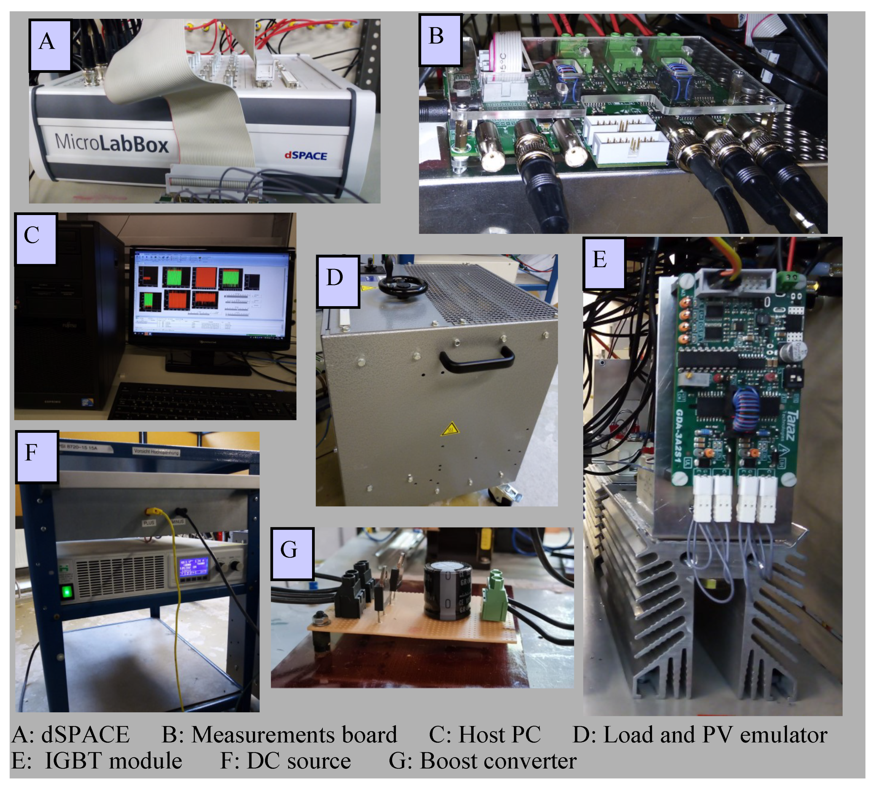
4.1. Test Bench Description

The system under consideration consists of a PV emulator, boost converter, two-level inverter, and inductive load. The PV emulator is constructed using DC source and group of resistors. Firstly, the DC source is connected with one resistor in series to emulate the P-V characteristics at a certain power level. After a period of time, another resistor is connected in parallel to the first one to emulate a sudden increase in power. Finally, the added resistor is removed to simulate an abrupt decrease in the output power of the emulator. Isolated voltage and current sensing module (USM-3IV) is used to measure the voltages and the currents. These measurements are fed to dSPACE DS1202 MicroLabBox, which is used as a real-time system. The control algorithm is developed using Matlab software, and hence, the generated switching state is applied to the switches. The smart gate drive module (GDA-2A2S1) is used as an interface between the dSPACE controller and the power switches. Figure 8 shows the experimental configuration of the set-up, while the specifications and components of the whole PV system are summarized in Table 2.

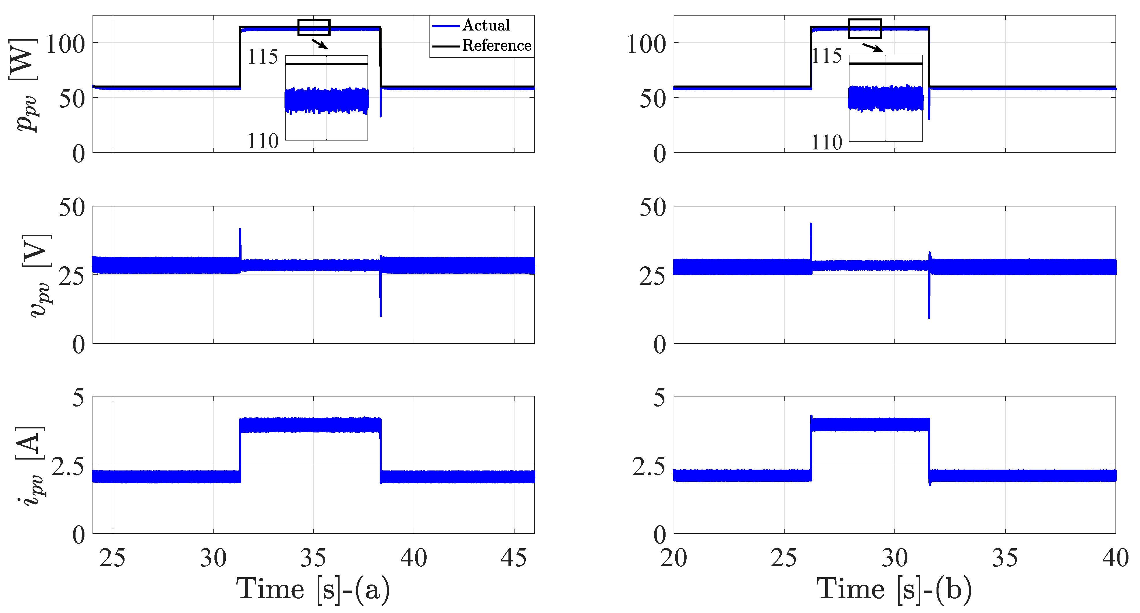
4.2. Evaluation of MPPT Behavior

In this subsection, the performance of the predictive fixed switching MPPT is investigated and compared with the P&O method. For fair comparison, an adaptive step-size is also utilized for the conventional P&O with the same constraints as of the predictive method. Figure 9 exhibits the results of the two methods, namely the predictive method and the P&O, where the PV power ( p p v ), voltage ( v p v ), and current ( i p v ) are shown, respectively. The two methods exhibit a very similar behavior at the step response of the PV emulator. However, the PV power with the proposed method gives a lower ripple content in the power waveform, which increases the efficiency. Furthermore, the tracking speed of the proposed method is faster than the P&O. Table 3 summarizes the behavior of the two methods regarding the average efficiency ( η p v , a v g ) and the tracking speed. It is worth mentioning that the average efficiency is calculated according to [27,28]. It seems that the average efficiency of the predictive method has a slight increase with respect to the conventional one. However, this value is calculated within a short span of time (range of seconds) as shown in the experimental results. Therefore, for a long time run, the energy utilization is expected to have a significant increase.
The duty cycle is examined in Figure 10, where the duty cycle with the adaptive step-size for the P&O method and the dual step-size for the predictive method are shown. It is obvious that the duty cycle with the P&O method has higher oscillations, especially at high power values. However, the duty cycle’s variation of the predictive technique is very tiny, and the duty cycle appears as a constant value. The reduced oscillation contributes to an enhanced waveform of the voltage and current, which results in an improved efficiency.
The behavior of the duty cycle is further investigated by inspecting the variations of the adaptive steps in the MPPT methods. For the two methods, the duty cycle is limited to a maximum change of 0.005 (saturation limit). This means that when an abrupt change happens, the duty cycle is limited to that value. This in turn has the benefit of limiting the oscillations of the voltages and currents at fast-changing atmospheric conditions. Additionally, and at steady state, if (at a certain operating point) the adaptive step-size is high, the oscillation of the duty cycle is restricted. Furthermore, the first step (corresponding to the current) of the predictive method is limited to 0.05 (saturation boundary).
Figure 11 shows the adaptive steps variation of the predictive method, where the first step ( Δ i ) and the second step ( Δ d ) are investigated. At the first interval, the current step-size variation is very small. This also applies to the corresponding duty cycle at the same interval. When a step-up change in the power occurs, the step-size of the current and duty cycle is saturated according to the predefined limits (0.05 and 0.005). At the second interval, the step-size variation of the current is a little bit higher in comparison to the first interval. However, the duty cycle variation remains approximately unchanged, thanks to the dual step-size design of the proposed method. Finally, when a step-down change (to the previous power level) in the power happens, the saturation limits are activated again, and the system goes into a steady state, similar to the first interval.
Figure 12 shows the step-size variation for the P&O method. It is quite obvious that the change of the duty cycle is remarkably large in comparison with the predictive technique. In the first and third intervals, the system succeeds to operate adaptively (under the saturation limit). However, at the second interval, the MPPT technique under P&O operates partially in the adaptive mode. In the zoomed part of the figure, the system operates at fixed step operation for certain operating points.

4.3. Inverter Control Results

Figure 13 presents the response of the inverter control with the conventional FS-MPC and the proposed efficient one, where the results show the DC-link voltage ( v d c ), the d-axis current ( i d ), the q-axis current ( i q ), and the injected three-phase currents ( i a b c ). The DC-link voltage exhibits over and undershoots in conjunction with the step changes of the PV power. However, the system returns quickly to the steady-state condition. As a consequence of the PV power change at the PV side, the d-axis current responds to that change to inject the excess power into the load. The q-axis current is maintained at its reference value ( i q r e f =0 for the unity power factor operation at grid-connected situation). Furthermore, the injected currents are sinusoidal.
As a result of the second objective of the inverter control (reduction of the switching frequency), the d-axis current and q-axis current reveal a slightly higher ripple. Therefore, the THD of the injected currents with the proposed method has a marginal increase evaluated against the conventional technique. To this end, Table 4 gives the values of the THD for the currents. It should be stated that the tuning procedure of the weighting factor is accomplished as discussed in [11].
The two methods are further evaluated according to the required computational load and average switching frequency ( f s ). Table 5 presents the calculated values with the help of the control desk program of the dSPACE controller. The execution time of the conventional FS-MPC is higher than the proposed one. Furthermore, the average switching frequency with the proposed method is decreased by approximately 10%. This percent can be increased by increasing the weighting factor value. However, this leads to a significant impact on the THD values.

5. Future Work

The current study proposed a predictive fixed switching MPPT strategy for the boost converter and a reduced complexity FS-MPC approach for the two-level inverter. However, the authors believe that the following points can be further discussed to enlighten the future directions in this aspect:
  • Investigation of the MPPT at dynamic operating conditions, in which the atmospheric conditions may have a slow or fast varying manner.
  • Comparative evaluation against the FS-MPC technique and other similar approaches for MPPT.
  • Further simplification for the FS-MPC to reduce its computational burden and include different control objectives.
  • Online adjustment of the weighting factor using intelligent techniques (optimization methods). Even more, elimination of the weighting factor in the cost function design to simplify the control objective and remove tuning efforts.
  • Robustness assessment and enhancement for the FS-MPC method. In this matter, analytical methods or observers can be utilized.
  • Implementing the control methodology with fewer sensors to improve the system’s reliability. In fact, these sensorless strategies can be an effective back-up during disturbances, noise, or even sensor failure.

6. Conclusions

In this paper, a predictive fixed switching MPPT is proposed, where two adaptive steps are designed to obtain the duty cycle of the boost converter. The first step is utilized during the prediction stage of the optimal voltage, whereas the second adaptive step is used to provide the duty cycle for the converter. Therefore, the conventional PI controller is eliminated, which simplifies the overall control strategy and reduces the tuning efforts. The proposed MPPT has higher efficiency and fast tracking speed in comparison with the conventional P&O. Furthermore, the conventional FS-MPC for inverter control is replaced with an efficient technique to reduce the computational load of the conventional method. In this technique, the polarity of the reference voltage is used as a guide of selectivity, where the switching vectors of the two-level inverter are sorted into two groups of positive and negative vectors. Based on that, only one set is considered for evaluation in the cost function design. This, in turn, reduces the possible computations of the cost function from 8 times with the conventional method to only 4 with the proposed one, which represents a 50% reduction. Moreover, the inverter control is modified to include the switching frequency reduction as an additional objective for the controller without any significant impact on the main one. In total, 10% reduction of the switching frequency is accomplished in our scheme. Future suggestions to improve the control performance include the elimination of the weighting factor and robustness enhancement.

Author Contributions

M.A. (Mostafa Ahmed) designed and implemented the proposed control strategy and wrote the manuscript. I.H. helped in writing the manuscript and the collection of the experimental results. M.A. (Mohamed Abdelrahem) revised and edited the manuscript. R.K. was responsible for the guidance and suggestions. All authors have read and agreed to the published version of the manuscript.

Funding

This research received no external funding.

Institutional Review Board Statement

Not applicable.

Informed Consent Statement

Not applicable.

Data Availability Statement

Not applicable.

Acknowledgments

This work was supported by the German Research Foundation (DFG) and the Technical University of Munich (TUM) in the framework of the Open Access Publishing Program.

Conflicts of Interest

The authors declare no conflict of interest.

References

  1. Owusu-Nyarko, I.; Elgenedy, M.A.; Abdelsalam, I.; Ahmed, K.H. Modified variable step-size incremental conductance MPPT technique for photovoltaic systems. Electronics 2021, 10, 2331. [Google Scholar] [CrossRef]
  2. Javed, M.Y.; Mirza, A.F.; Hasan, A.; Rizvi, S.T.H.; Ling, Q.; Gulzar, M.M.; Safder, M.U.; Mansoor, M. A comprehensive review on a PV based system to harvest maximum power. Electronics 2019, 8, 1480. [Google Scholar] [CrossRef] [Green Version]
  3. Bayod-Rújula, Á.A.; Cebollero-Abián, J.A. A novel MPPT method for PV systems with irradiance measurement. Sol. Energy 2014, 109, 95–104. [Google Scholar] [CrossRef]
  4. Eltamaly, A.M.; Farh, H.M.H.; Othman, M.F. A novel evaluation index for the photovoltaic maximum power point tracker techniques. Sol. Energy 2018, 174, 940–956. [Google Scholar] [CrossRef]
  5. De Brito, M.A.G.; Galotto, L.; Sampaio, L.P.; Melo, G.d.A.; Canesin, C.A. Evaluation of the main MPPT techniques for photovoltaic applications. IEEE Trans. Ind. Electron. 2012, 60, 1156–1167. [Google Scholar] [CrossRef]
  6. Bhatnagar, P.; Nema, R.K. Maximum power point tracking control techniques: State-of-the-art in photovoltaic applications. Renew. Sustain. Energy Rev. 2013, 23, 224–241. [Google Scholar] [CrossRef]
  7. Ram, J.P.; Babu, T.S.; Rajasekar, N. A comprehensive review on solar PV maximum power point tracking techniques. Renew. Sustain. Energy Rev. 2017, 67, 826–847. [Google Scholar] [CrossRef]
  8. Elgendy, M.A.; Zahawi, B.; Atkinson, D.J. Analysis of the performance of DC photovoltaic pumping systems with maximum power point tracking. In Proceedings of the 4th IET International Conference on Power Electronics, Machines and Drives (PEMD 2008), York, UK, 2–4 April 2008; pp. 426–430. [Google Scholar]
  9. Ahmed, M.; Abdelrahem, M.; Kennel, R. Highly efficient and robust grid connected photovoltaic system based model predictive control with kalman filtering capability. Sustainability 2020, 12, 4542. [Google Scholar] [CrossRef]
  10. Ahmed, M.; Abdelrahem, M.; Harbi, I.; Kennel, R. An Adaptive Model-Based MPPT Technique with Drift-Avoidance for Grid-Connected PV Systems. Energies 2020, 13, 6656. [Google Scholar] [CrossRef]
  11. Ahmed, M.; Harbi, I.; Kennel, R.; Abdelrahem, M. Dual-Mode Power Operation for Grid-Connected PV Systems with Adaptive DC-link Controller. Arab. J. Sci. Eng. 2021, 1–15. [Google Scholar] [CrossRef]
  12. Kakosimos, P.E.; Kladas, A.G. Implementation of photovoltaic array MPPT through fixed step predictive control technique. Renew. Energy 2011, 36, 2508–2514. [Google Scholar] [CrossRef]
  13. Shadmand, M.; Balog, R.S.; Rub, H.A. Maximum Power Point Tracking using Model Predictive Control of a flyback converter for photovoltaic applications. In Proceedings of the 2014 Power and Energy Conference at Illinois (PECI), Champaign, IL, USA, 28 February–1 March 2014; pp. 1–5. [Google Scholar]
  14. Metry, M.; Shadmand, M.B.; Balog, R.S.; Abu-Rub, H. MPPT of photovoltaic systems using sensorless current-based model predictive control. IEEE Trans. Ind. Appl. 2016, 53, 1157–1167. [Google Scholar] [CrossRef]
  15. Mosa, M.; Shadmand, M.B.; Balog, R.S.; Rub, H.A. Efficient maximum power point tracking using model predictive control for photovoltaic systems under dynamic weather condition. IET Renew. Power Gener. 2017, 11, 1401–1409. [Google Scholar] [CrossRef]
  16. Sajadian, S.; Ahmadi, R. Model predictive-based maximum power point tracking for grid-tied photovoltaic applications using a Z-source inverter. IEEE Trans. Power Electron. 2016, 31, 7611–7620. [Google Scholar] [CrossRef]
  17. Abushaiba, A.A.; Eshtaiwi, S.M.M.; Ahmadi, R. A new model predictive based maximum power point tracking method for photovoltaic applications. In Proceedings of the 2016 IEEE International Conference on Electro Information Technology (EIT), Grand Forks, ND, USA, 19–21 May 2016; pp. 0571–0575. [Google Scholar]
  18. Abdel-Rahim, O.; Alamir, N.; Abdelrahem, M.; Orabi, M.; Kennel, R.; Ismeil, M.A. A phase-shift-modulated LLC-Resonant micro-inverter based on fixed frequency predictive-MPPT. Energies 2020, 13, 1460. [Google Scholar] [CrossRef] [Green Version]
  19. Manoharan, P.; Subramaniam, U.; Babu, T.S.; Padmanaban, S.; Holm-Nielsen, J.B.; Mitolo, M.; Ravichandran, S. Improved perturb and observation maximum power point tracking technique for solar photovoltaic power generation systems. IEEE Syst. J. 2020, 15, 3024–3035. [Google Scholar] [CrossRef]
  20. Bhattacharyya, S.; Samanta, S.; Mishra, S. Steady Output and Fast Tracking MPPT (SOFT-MPPT) for P&O and InC Algorithms. IEEE Trans. Sustain. Energy 2020, 12, 293–302. [Google Scholar]
  21. Liu, F.; Duan, S.; Liu, F.; Liu, B.; Kang, Y. A variable step size INC MPPT method for PV systems. IEEE Trans. Ind. Electron. 2008, 55, 2622–2628. [Google Scholar]
  22. Killi, M.; Samanta, S. Modified perturb and observe MPPT algorithm for drift avoidance in photovoltaic systems. IEEE Trans. Ind. Electron. 2015, 62, 5549–5559. [Google Scholar] [CrossRef]
  23. Shongwe, S.; Hanif, M. Comparative analysis of different single-diode PV modeling methods. IEEE J. Photovoltaics 2015, 5, 938–946. [Google Scholar] [CrossRef]
  24. Chouder, A.; Silvestre, S.; Sadaoui, N.; Rahmani, L. Modeling and simulation of a grid connected PV system based on the evaluation of main PV module parameters. Simul. Model. Pract. Theory 2012, 20, 46–58. [Google Scholar] [CrossRef]
  25. Bellia, H.; Youcef, R.; Fatima, M. A detailed modeling of photovoltaic module using MATLAB. NRIAG J. Astron. Geophys. 2014, 3, 53–61. [Google Scholar] [CrossRef] [Green Version]
  26. Rodriguez, J.; Garcia, C.; Mora, A.; Flores-Bahamonde, F.; Acuna, P.; Novak, M.; Zhang, Y.; Tarisciotti, L.; Davari, A.; Zhang, Z.; et al. Latest Advances of Model Predictive Control in Electrical Drives. Part I: Basic Concepts and Advanced Strategies. IEEE Trans. Power Electron. 2021. [Google Scholar] [CrossRef]
  27. Ahmed, J.; Salam, Z. An improved perturb and observe (P&O) maximum power point tracking (MPPT) algorithm for higher efficiency. Appl. Energy 2015, 150, 97–108. [Google Scholar]
  28. Ahmed, J.; Salam, Z. A modified P&O maximum power point tracking method with reduced steady-state oscillation and improved tracking efficiency. IEEE Trans. Sustain. Energy 2016, 7, 1506–1515. [Google Scholar]
Figure 1. P-V characteristics of the PV source under different radiation conditions.
Electronics 10 03109 g001
Figure 2. I–V characteristics of the PV source under different radiation conditions.
Electronics 10 03109 g002
Figure 3. Equivalent circuit of the boost converter when: (a) switch is OFF, and (b) switch is ON.
Electronics 10 03109 g003
Figure 4. (a) Two-level voltage source inverter with grid connection. (b) Switching states and voltage vectors of the inverter.
Electronics 10 03109 g004
Figure 5. The simplified equivalent circuit of the PV source.
Electronics 10 03109 g005
Figure 6. The flowchart of the proposed predictive MPPT technique.
Electronics 10 03109 g006
Figure 7. The configuration and proposed control strategy for the two-stage PV system.
Electronics 10 03109 g007
Figure 8. The experimental set-up of the two-stage PV system.
Electronics 10 03109 g008
Figure 9. The behavior of the MPPT techniques: (a) Conventional P&O method with adaptive step-size; (b) proposed predictive method with two adaptive step-size.
Electronics 10 03109 g009
Figure 10. The duty cycle command of the boost converter: (a) Conventional P&O method with adaptive step-size and (b) proposed predictive method with two adaptive step-size.
Electronics 10 03109 g010
Figure 11. Variation of the adaptive step-size of the proposed predictive method: (a) current step-size and (b) duty cycle step-size.
Electronics 10 03109 g011
Figure 12. Variation of the duty cycle step-size with the conventional P&O technique.
Electronics 10 03109 g012
Figure 13. Performance of the inverter control: (a) conventional FS-MPC and (b) The proposed FS-MPC with switching frequency minimization.
Electronics 10 03109 g013
Table 1. Switching actions and output voltages of the two-level inverter in α β and a b c frames.
Voltage VectorsSwitching States ( S abc ) Output Voltages ( u α , u β ) Output Voltages ( u a , u b , u c )
u 0 0000 00 0 0
u 1 100 2 v d c 3 0 2 v d c 3 v d c 3 v d c 3
u 2 110 v d c 3 3 v d c 3 v d c 3 v d c 3 2 v d c 3
u 3 010 v d c 3 3 v d c 3 v d c 3 2 v d c 3 v d c 3
u 4 011 2 v d c 3 0 2 v d c 3 v d c 3 v d c 3
u 5 001 v d c 3 3 v d c 3 v d c 3 v d c 3 2 v d c 3
u 6 101 v d c 3 3 v d c 3 v d c 3 2 v d c 3 v d c 3
u 7 1110 00 0 0
Table 2. PV system parameters.
ParameterValue
Boost inductance ( L ) 8.5 mH
Output capacitor ( c d c ) 240 μ F
Power switchsingle switch (IGBT-Module FF50R12RT4)
Diode ( D ) fast recovery diode BYW77PI200
DC-link reference voltage ( v d c r e f ) 50 V
Load resistance ( R l ) 5 Ω
Load inductance ( L l ) 11 mH
PV emulator resistors 15 Ω / 16.5 Ω
Sampling time ( T s ) 100 μ s
Table 3. Tracking speed and average efficiency of the MPPT techniques.
MethodTracking Speed η pv , avg (%)
P&O with adaptive step-size7 T s 97.45
Predictive method with two adaptive step-size5 T s 97.51
Table 4. THD of the a b c currents with the conventional and proposed method.
MethodTHD %
Conventional (low/high power)4.53/3.42
Proposed (low/high power)4.68/3.44
Table 5. Execution time and average switching frequency for inverter control techniques.
MethodExecution Time ( μ s)Avg. f s (kHz)
Conventional method15.342.26
Proposed technique12.552.04
Publisher’s Note: MDPI stays neutral with regard to jurisdictional claims in published maps and institutional affiliations.

