Enhancing Big Data Feature Selection Using a Hybrid Correlation-Based Feature Selection

Abstract

This study proposes an alternate data extraction method that combines three well-known feature selection methods for handling large and problematic datasets: the correlation-based feature selection (CFS), best first search (BFS), and dominance-based rough set approach (DRSA) methods. This study aims to enhance the classifier’s performance in decision analysis by eliminating uncorrelated and inconsistent data values. The proposed method, named CFS-DRSA, comprises several phases executed in sequence, with the main phases incorporating two crucial feature extraction tasks. Data reduction is first, which implements a CFS method with a BFS algorithm. Secondly, a data selection process applies a DRSA to generate the optimized dataset. Therefore, this study aims to solve the computational time complexity and increase the classification accuracy. Several datasets with various characteristics and volumes were used in the experimental process to evaluate the proposed method’s credibility. The method’s performance was validated using standard evaluation measures and benchmarked with other established methods such as deep learning (DL). Overall, the proposed work proved that it could assist the classifier in returning a significant result, with an accuracy rate of 82.1% for the neural network (NN) classifier, compared to the support vector machine (SVM), which returned 66.5% and 49.96% for DL. The one-way analysis of variance (ANOVA) statistical result indicates that the proposed method is an alternative extraction tool for those with difficulties acquiring expensive big data analysis tools and those who are new to the data analysis field.

1. Introduction

Uncertainty is one of the main problems in data analysis, as datasets consisting of this kind of problem might generate incorrect decisions. Uncertainty can be divided into two categories; internal and external. Internal uncertainty is generated by decision-makers that deal with the data during the analysis process. An example of internal uncertainty is related to the factors or preferences defined by the decision-makers. On the other hand, external uncertainty is the value that has been identified earlier during data collection. However, it needs to be re-analysed by assessing the incoming situation to predict the correct value.

Normally, many researchers prefer to solve internal uncertainty problems that mostly deal with complex information [1]. For example, Zhang et al. proposed a new method for fuzzy information which was developed with inspiration from the PROMETHEE method. The method uses fuzzy rough sets by [2] and a decision-making hybrid method called Intuitionistic fuzzy N-soft rough sets (IFNSRSs), which solves the problem of uncertainty [3]. However, the uncertainty problem might affect the decision-making process by causing inconsistent and imprecise decisions [4]. Therefore, uncertainty values need to be processed or analysed. Various methods and algorithms have been proposed to solve the uncertainty problem. One of the more effective methods, known as the feature selection method, is used to eliminate the uncertainty in a dataset. Some of the well-known methods include the fuzzy set theory, probability theory and approximation theory. These methods have proven efficiency when implemented in assisting the decision method, such as the ‘classifier’ in the decision analysis process. A list of methods, especially on feature selection, have been mentioned by [5], in their survey paper; the Bayesian inference method and the Information-theoretic ranking criteria filtering method. However, not all the proposed works were capable of dealing with different kinds of data and problems. Some of the works were specifically constructed to improvise the fundamental theory [6,7], while others constructed the hybridised methods to overcome the unresolved problems, especially in the feature selection process [8,9].

The majority of the proposed feature selection methods considered the characteristics and failed to focus on the volume of the datasets. Therefore, most of the methods had difficulty dealing with big datasets and suffered from memory space and computing time problems. Deep learning (DL) is one method capable of handling big data, especially for classification and recognition processes. It uses a pre-training and fine-tuning process to identify the most optimised attribute set to use in the decision-making task. The DL model that was commonly used for big data features analysis is a reliable DL model used for low-quality data, incremental DL models for real-time data, large-scale DL models for big data, multi-modal DL model and deep computation models for heterogeneous data [10]. Other than DL, artificial bee colony (ABC) with MapReduce has been proposed to deal with big datasets, whereas ABC was used to select the features and MapReduce was used to deal with the large volume of data [11]. Additionally, random forest (RF), which is one of the statistical methods, is also well-known for use in selecting the features of big datasets. Several variants of RF were proposed, such as sequential RF (seqRF), parallel computation of RF (parRF), sampling RF (sampRF), m-out-of-n RF (moonRF), bag of little bootstraps RF (blbRF), divide-and-conquer RF (dacRF) and online RF (onRF) [12]. Several feature selection methods require parallel architecture and high performance computing to be successfully executed. Otherwise, it might increase the cost of hardware and software. For instance, large memory space and effective software like Hadoop MapReduce are needed for the learning and analysis process.

Motivated by the highlighted problems: (i) uncertainty and (ii) large datasets, this paper suggests an alternative hybrid method in the big data extraction process by integrating two well-known single methods in handling the uncertainty problem and large data size issue: Correlation-based feature selection (CFS) and the dominance-based rough set approach (DRSA). Both methods are well-known in identifying the most optimised features where CFS will identify the important features based on the correlation value on each feature with its defined class and can increase the classification performance. Meanwhile, DRSA, an extension of rough set theory, was commonly used to handle uncertainty values by considering the logical inference between an attribute and its defined class. To the best of our knowledge, only a few works have applied single or enhanced CFS and DRSA or the combination of these two methods in handling big datasets with uncertainty problems. Some more recent works that used CFS and DRSA in handling big datasets are from [13,14] including our previous work combining CFS with the rough set [15].

This proposed method intends to assess the capability of the combination of CFS and DRSA to assist the classifier in developing the optimized attribute set. CFS will be used to reduce the uncorrelated attributes. Meanwhile, DRSA will eliminate the uncertainty data values in the datasets during the data analysis process. The proposed method will act as a feature selection method for raw datasets, so a cleaned or optimized dataset could be provided to the classifier. Due to the excellent performance of both CFS and DRSA in handling multi-value datasets on many research works, this proposed work tries to combine both methods to achieve a high-performance accuracy rate. This work also tries to evaluate the behavior of the applied datasets that consist of different characteristics after going through the feature selection process and whether they are still effective to be classified.

This proposed work has contributed in two issues associated with big data which are large data volumes, and the different variety of datasets. CFS-DRSA is capable in handling multivalue and large datasets and become one of the effective feature selection methods. Due to this, it also can be implemented in various fields such as healthcare and business operation. The proposed operational framework can be used as a guideline to the decision makers especially in the same area.

Several sections have been built to address the whole phase of the proposed work. Section 1 introduces the main issues that need to be discussed. Section 2 presents several essential concepts on the DRSA method, the feature reduction method, the correlation-based feature selection method (CFS), the support vector machine (SVM), and the recent works related to the DRSA feature selection method. Section 3 elaborates further on the execution of the feature extraction and selection process in the proposed method, followed by Section 4 discusses the experimental work and obtained results. Finally, Section 5 concludes the proposed method with recommendations for future work.

2. Related Works

Several essential terms and concepts are discussed in this section, including the feature reduction method, the DRSA method, the correlation-based feature selection (CFS) method, the support vector machine (SVM) and the recent hybrid feature selection methods. Explaining these terms and concepts will indirectly increase the user’s understanding of the aspects that will be addressed and highlighted in the proposed method.

2.1. Feature Reduction Method

The feature reduction method is a technique used to eliminate attributes defined by decision-makers using selected algorithms such as the ‘soft set parameter reduction algorithm’ [16] and the ‘best first search algorithm’ [17]. It can also help decision-makers to analyse and identify the set of important attributes in the datasets [18]. The feature reduction method, also known as ‘attribute reduction’ or ‘feature extraction’ in some application areas, is implemented in the pre-processing phase as the data need to be cleaned from any issue. Different approaches have been introduced and implemented by researchers. The well-known approaches are based on the correlation between the attribute that selects the highly relevant features in the available dataset such as the correlation-based feature selection (CFS) [19], maximal discernibility pairs, Gaussian kernel, fuzzy rough sets [5], and measuring dependency through the Chromosomal fitness score like the rough set-based genetic algorithm and Rough sets-based incremental calculation dependency [20].

The feature reduction process result is an optimised reduction set that will be used in the data analysis phase. It helps the analysis method, such as the classifier and prediction method, in producing the best solution. Many research works have proved that decisions can be made effectively with feature reduction assistance, and problems easily solved [21]. RST, soft set theory (SST), and fuzzy set theory (FST) are among the most effective feature reduction methods in dealing with uncertainty and inconsistency problems [22,23]. These theories have inspired many researchers to produce new theories that solve different kinds of data problems.

2.2. Rough Set Theory (Rst)

Rough set theory (RST) is one of the outperforming feature reduction methods widely used in research. Pawlak initiated in 1997, using a mathematical approach in dealing with uncertainty, imprecision, and vagueness [24]. The basic concept of the rough set is defined as:

Definition 1.

If the universe set U is a non-empty finite set and σ is an equivalence relation on U. Then, $(U,\sigma )$ is called an approximation space. If X is a subset of U, X either can be written or not as a union of the equivalence classes of U. X is definable if it can be written as a union of some equivalence classes of U or else it is not definable. If X is not definable, it can be approximated into two definable subsets called lower and upper approximations of X as shown below [9,25].

• $\underline{app}\left(X\right)$ = $\bigcup \{{\left[x\right]}_{\sigma }:{\left[x\right]}_{\sigma }\subseteq X\}$,
• $\overline{app}\left(X\right)$ = $\bigcup \{{\left[x\right]}_{\sigma }:{\left[x\right]}_{\sigma }\cap X\ne \varnothing \}$.

A rough set is comprised of $(\underline{app}\left(X\right),\overline{app}\left(X\right))$. Boundary region is when the set $\overline{app}\left(X\right)$–$\underline{app}\left(X\right)$. Therefore, if $\underline{app}\left(X\right)$ = $\overline{app}\left(X\right)$, X is definable. If $\overline{app}\left(X\right)$–$\underline{app}\left(X\right)$, then X is an empty set.

For a set of X, $\underline{app}\left(X\right)$ is the greatest definable set contained in X, whereas $\overline{app}\left(X\right)$ is the least definable set containing X.

In the decision-making process and especially in the feature reduction task, the RST theory promotes several advantages, such as searching vague data, making the algorithm easily understandable and managing a large size of datasets [24]. Some works have proposed research frameworks involving RST, enhancing the fundamental theory according to the specific area, while some of the other works integrated the RST with other theories or methods to enhance the capability of each combination [26,27,28]. For example, the dominance-based rough set (DRSA) [29], the variable precision dominance-based rough set (VP-DRSA) [30], fuzzy rough set model [5], fuzzy soft sets and rough sets [16] and the trapezoidal fuzzy soft set [31].

DRSA has been widely used in solving uncertainty and inconsistency problems, proposed specifically to deal with ordinal datasets. Motivated by these existing works and with little focus on the expansion of the DRSA, this paper aims to extend the previous work on the DRSA and evaluate the performance of the proposed hybrid DRSA method in dealing with high volumes and dataset varieties. In addition, this paper also conducts several experiments on the nominal dataset to evaluate the ability of DRSA to analyse other types of data instead of the ordinal type. The experimental work outcome is expected to bring favourable performance results of the two main processes at the data reduction phase and data selection phase.

2.3. Dominance-Based Rough Set Approach (Drsa)

DRSA was an extension of the classical rough set approach (CRSA) and was inspired by Pawlak’s work [32]. In 2010, Greco et al., extended the CRSA to address and overcome the limitation in dealing with nominal data only. Moreover, only the classification process could be handled by the CRSA. The specific function of the DRSA is to deal with ordinal data; however, it also can be used in dealing with other types of datasets. Due to the multiple abilities of DRSA in handling different kinds of criteria in the dataset, it is also known as the ‘multi-attribute criteria method’. In the data analysis process, the selection concept "if:else" has been used since the data must go through with two essential conditions before it is assigned to the specific value. During the analysis process, the attribute that represents the condition will be set as ‘criteria’ that need to be analysed, and the attribute that represents the decision will be set as ‘ordered preferences’ or pre-defined classes. The knowledge, which is also known as ‘dominance relation’ will be presented as sets of objects and classes that consist of the integration of several sets of upper and lower classes.

Normally, DRSA presents the data in a decision table format. The result of the analysis process is in the reduction of the set list where the reduction set can be of more than one value. In addition, the intersection of the row and column in the table represents the value, which is important in the analysis process. Thus, the decision rules can be created by calculating the approximation between the upper and lower classes’ values. Classification, optimisation, and ranking are the only three tasks that DRSA can solve [33]. Five requirements must be followed when producing the rules of decision based on real, probable, and approximate conditions between $D_{\ge }$ -decision rules and objects x [29]:

• Certain $D_{\ge }$ -decision rules, have lower profile details for objects owned by $C{l}_t^{\ge }$ without ambiguity.
• Possible $D_{\ge }$ -decision rules, have lower profile details for objects owned by $C{l}_t^{\ge }$ with or without ambiguity.
• Certain $D_{\le }$ -decision rules, have upper profile details for objects owned by $C{l}_t^{\le }$ without ambiguity.
• Possible $D_{\le }$ -decision rules, have upper profile details for objects owned by $C{l}_t^{\le }$ with or without any ambiguity.
• Approximate $D_{\le \ge }$ -decision rules, have concurrently lower and upper profile details for objects owned by $C{l}_s\cup C{l}_{s+1}\cup ...\cup C{l}_t$ without possibility of discerning the class.

The certain rule indicates that only certain information will be processed from the original dataset, while the possible rule indicates possible information, and the approximate rule indicates uncertainty information.

2.4. Correlation-Based Feature Selection (Cfs) Method

The correlation-based feature selection method, also known as CFS, is one method that can select the best features of a big dataset. The CFS will identify the best feature based on the association, firstly between the features and their paired features, and secondly between features and their defined category.

The formula to identify the most correlate attribute in the dataset is shown in Equation (1) [34].

$$c{r}_{zc}=\frac{f\overline{c{r}_{zi}}}{\sqrt{f+f(f-1)\overline{c{r}_{ii}}}}$$

(1)

where $c{r}_{zc}$ is the heuristic value of a subset attribute for f number of attributes, $\overline{c{r}_{zi}}$ represents the average value of correlations between the attributes and the class, and $\overline{c{r}_{ii}}$ holds the average value of inter-correlation between attribute pairs. To reduce data dimensionality, the subset with the highest $c{r}_{zc}$ value is utilized.

Importantly, CFS is one of the multivariate feature selection methods that implement a heuristic search to analyse the best features to be used in the dataset. The best features are chosen based on the level and the significant correlation value between the feature and its class [34]. Accordingly, this ability makes CFS one of the most widely used methods implemented in the feature extraction process, especially in big data application areas. Notwithstanding, CFS has also shown many significant results that aid decision-makers in improving the decision analysis process’s performance.

The main advantage of CFS is that it requires less computational complexity compared to Wrappers and other approaches. However, the performance of the learning algorithm is not as promising as wrappers and embedded approaches. Thus, many researchers took the initiative to improvise and enhance CFS’s capability by integrating it with other feature selection methods. For instance, a combination of CFS and BFS where CFS acts as an attribute evaluator and BFS acts as a searching method in the attribute analysis process [35]. CFS has been widely implemented to deal with many applications such as to solve the issue of high dimensional data [36] and parallel computing [13], complex datasets [35] and medical [37,38]. It is recently reported that CFS helped the decision-makers increase the decision-making performance by optimising the capability of the existing decision analysis methods and became one of the frequently used feature selection methods [39].

2.5. Best First Search (Bfs)

The BFS is based on a heuristic search algorithm that deals with open and closed lists of the node tree. An open list represents the front node, while a closed list represents the extended node tree. Each node has its own unique value and is evaluated using a cost function value. The algorithm will be ended when the goal node is found. Normally, the goal node will be selected if the cost function returns at a minimum cost value [40]. Breadth-first search, Dijkstra’s single-source shortest-path algorithm, and the A* algorithm are several examples of BFS methods [41]. These algorithms are different in terms of cost function calculation. If the cost function is related to the depth of the node in the tree, the best first search is defined as a breadth-first search. This algorithm will focus on the specified depth first then followed by extending the value into greater depth. If the tree has a different cost value of edges and the node $\left(n\right)$ cost is $g\left(n\right)$, then the sum of the edge costs starting from the root to node n is defined as Dijkstra’s single-source shortest-path algorithm.

Meanwhile, the A* algorithm is the extension of Dijkstra’s single source shortest-path algorithm by adding the cost function to heuristic cost estimation $h\left(n\right)$ from node n to the goal node; A* algorithm will return the minimum cost result if the $h\left(n\right)$ never exceeds the actual cost of node n to the goal. The definition of the A* algorithm is as follows, $f\left(n\right)=g\left(n\right)+h\left(n\right)$ where n represented as the node. BFS is one of the most used search-based algorithms and is able to return lower bound feed-back of data values quickly, at the expense of wasteful reconstruction of discarded solutions [17]. In other words, BFS provide the output based on the lower bound value of the available solutions within the search nodes [42]. However, BFS suffers from memory complexity when dealing with large datasets. Surprisingly, it returns good results when combined with CFS selection method from the previous experimental work compared to other search algorithms like the genetic algorithm and genetic search [15]. Thus, this study will combine the previous work between CFS and BFS with another outstanding feature selection method, DRSA.

2.6. Support Vector Machine (Svm)

A support vector machine (SVM) is one of the machine learning tools used to analyse a dataset’s features. SVM analyses the features of the dataset found on a hyperplane or line weightage value. The most effective hyperplane is one that exhibits the most significant value and its global value. Therefore, the SVM is capable of identifying non-linear relationships among datasets [43]. Moreover, it is a popular supervised learning algorithm typically used as a classifier, returning good results in the decision analysis process. Some of the application fields that have taken advantage of their capabilities are face prediction, text classification, engineering, and the statistic and learning theory [44,45].

2.7. Recent Works Related to the Drsa Feature Selection Method

A variety of new DRSA approaches have been proposed, given the weakness of the existing DRSA system. For example, Reference [6], suggested enhancing fundamental DRSA, making it possible for the original DRSA to manage nominal attributes by including information from the decision table. Compared with other traditional rule-based methods, this method has successfully returned high classification results. Reference [33], proposed a new extension of DRSA for handling composite ordered data that consisted of multiple types of data, which are dynamic maintenance of the lower and upper approximations under the attribute generalisation, missing attributes, numerical, interval-valued and categorical. The proposed work improved the processing time compared to the non-incremental method. Reference [46], modified the complexity of the conventional DRSA approach by proposing new algorithms to calculate the upper and lower approximation; thus, reducing 50% of the processing time. DRSA also inspired Huang et al., to combine the dominance-based and multi-scale intuitionistic fuzzy (IF) approach to represent multi-level data structures in a decision table. The results of this study have generalised the fundamental approach of rough set theories and the DRSA itself so that a new multi-scale approach named multi-scale dominance-based intuitionistic decision table (MS-DIFDT) was proposed in selecting an optimal set of data [47]. Furthermore, some of the researchers preferred to use DRSA as a method of analysis. For example, Reference [48], proposed a method that could combat poverty. Reference [49] proposed an analysis method that could examine employees’ perception in the workplace, while Reference [50] suggested a work that could deal with incomplete ordered information systems.

2.8. Existing Works on Feature Selection Methods

Rough set and fuzzy set theories are examples of the methods that have failed to become a good parameterisation tool, and it has been proven by Molodtsov, who proposed an SST to overcome the issue of parameterisation incompatibility. However, the limitation of the existing parameterisation methods depends on certain factors, such as the improper selection of hardware and software. Not only rough set and fuzzy set theories difficulties, but other parameterisation methods are also experiencing difficulties in analysing the large size of data that have caused the need for significant memory space and resulting in long processing time. The following item and Table 1 presents the advantages and disadvantages of previous works on hybrid feature selection methods.

• Fuzzy rough sets feature selection method [51] is used as a feature selection method based on fuzzy divergence measure. However, it requires a long processing time for large size datasets.
• Multi-label fuzzy rough set (MLFRS) method [52]. This method was proposed for multi-label learning and is able to identify the exact different classes’ samples based on the whole label space. It can also obtain robust upper and lower approximations of the datasets and outperformed when compared to other state-the-art algorithms. It performed better when using larger data instead of 5000 samples for each dataset.
• Novel fuzzy rough set methods based on the PROMETHEE method [2]. It is a dynamic method able to solve complex multi-criteria decision-making problems. It is scalable and capable of solving complex criteria; however, the proposed method is only applicable to a single decision-maker and not applicable for group decision-making.
• Fuzzy parameterised complex multi-fuzzy soft set (FPCMFS-set) [53]. It was proposed to improve the existing method by adding the time frame in analysing multi-dimensional data by providing the basic notation on complement, union, and intersection operations. However, the proposed work only provides the proof of the definitions without testing any real-world dataset.
• Soft dominance-based rough sets [54]. It was proposed to improve Pawlak’s and Sun’s methods in solving multi-agent conflict analysis decision problems. Overall, the proposed method only performs benchmarking on Sun’s method and on labour management negotiation problems.
• Hybrid fuzzy multi-criteria decision methodology model using best-worst method (BWM) and MARCOS (measurement alternatives and ranking according to copromise solution) approaches. This work is proposed to rank the list of the appropriate hydrogen solutions for public transport with buses [55]. This work only tested the proposed model on certain type of data.
• Weighted aggregated sum product assessment (WASPAS) approach based on the fuzzy Hamacher weighted averaging (FHWAA) function and weighted geometric averaging (FHWGA) function to rank the supply chain and sustainability measures. This work also focused on specific data which is on electric ferry [56].

Table 1. Other existing works on hybrid feature selection methods.

Fuzzy parameterized complex multi-fuzzy soft set (FPCMFS-set) [53].	It was an enhancement of fuzzy parameterized fuzzy soft set that was initiated to improve the analysis work towards multi-dimensional data. Several mathematical operations had been defined such as intersection, union and complement to prove the proposed concept. However, the concept has not being tested to any example or any real world dataset as validation process.
Integration of fuzzy and soft set theories [57].	This work was proposed to construct an expert system in diagnosing the survival for lung cancer patients. The integrated theories were used to analyze clinical and functional data by fuzzifying the raw data and generating the soft decision rules to predict the surgical risk of lung cancer patients. The obtained results showed that the proposed work had achieved 79% of classification accuracy rate which was quite efficient for survivor rate prediction.
An integrated method of deep learning and support vector machine [58].	This work was proposed to forecast corporate failure in the Chinese energy Sector. Soft set was applied as an output integrator between convolutional neural network oriented deep learning (CNN-DL) and support vector machine (SVM) classifiers. The proposed method had performed well and able to improve the performance of the forecasting process.

Table 1. Other existing works on hybrid feature selection methods.

Fuzzy parameterized complex multi-fuzzy soft set (FPCMFS-set) [53].	It was an enhancement of fuzzy parameterized fuzzy soft set that was initiated to improve the analysis work towards multi-dimensional data. Several mathematical operations had been defined such as intersection, union and complement to prove the proposed concept. However, the concept has not being tested to any example or any real world dataset as validation process.
Integration of fuzzy and soft set theories [57].	This work was proposed to construct an expert system in diagnosing the survival for lung cancer patients. The integrated theories were used to analyze clinical and functional data by fuzzifying the raw data and generating the soft decision rules to predict the surgical risk of lung cancer patients. The obtained results showed that the proposed work had achieved 79% of classification accuracy rate which was quite efficient for survivor rate prediction.
An integrated method of deep learning and support vector machine [58].	This work was proposed to forecast corporate failure in the Chinese energy Sector. Soft set was applied as an output integrator between convolutional neural network oriented deep learning (CNN-DL) and support vector machine (SVM) classifiers. The proposed method had performed well and able to improve the performance of the forecasting process.

Overall, there are three main problems faced by the existing parameterisation methods: (i) not all parameterisation methods are able to provide the most optimal and sub-optimal parameters. This is because of the capability of each method in computing various kinds of datasets [59], (ii) most of the methods are NP hard problems and suffered from great amount of computation work. This problem occurs when the methods are dealing with large sized datasets. Many derivations on mathematical formulations need to be stored in computer memory; thus, the desired problem was unable to be solved [5], (iii) memory consumption and computation time to analyse the most optimal and sub-optimal parameters especially on big data. Most of the methods require huge memory and more time in analysing big datasets [60,61]. These problems occurred due to the complexity of the problems and datasets, the dimension of the dataset, and the software and hardware used during the decision analysis process.

3. Proposed Work: Hybrid Correlation-Based Feature Selection

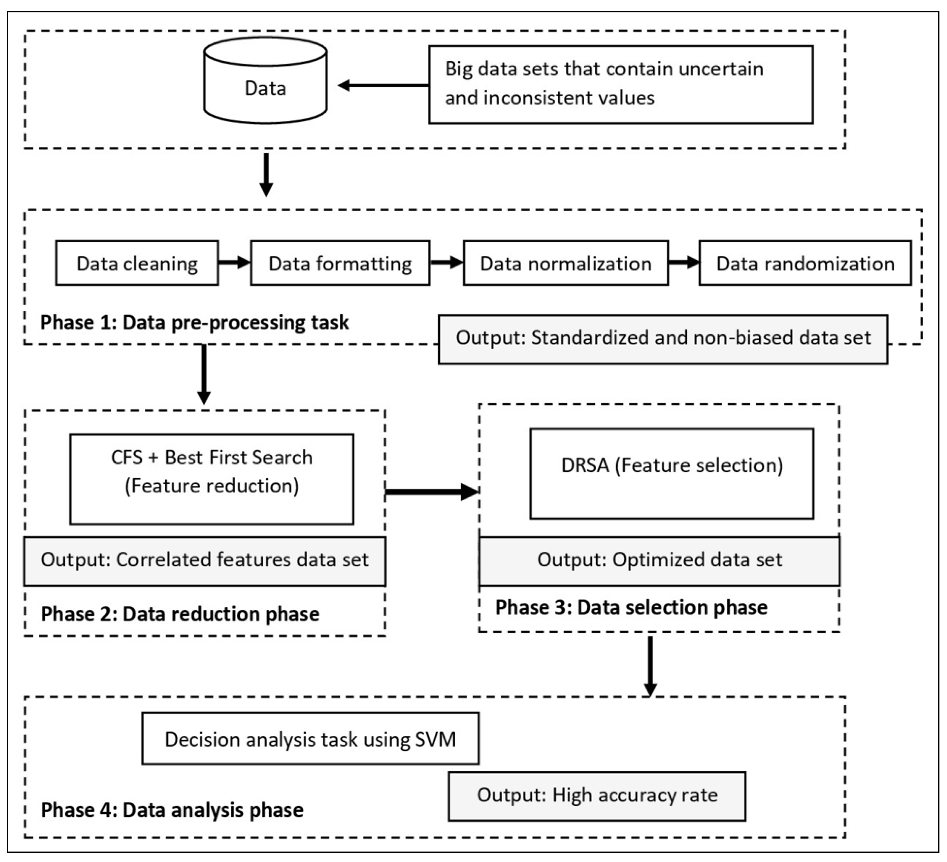
In this section, we describe the proposed hybrid correlation-based feature selection model. The model consisted of two main phases: the data reduction phase and the data selection phase. Several processes were employed to support these two phases: data pre-processing and data analysis. The purpose of developing this framework was to develop a hybrid feature selection method to deal with uncertain data of large volumes. The hybrid aspect was at the data reduction and data selection phases; these two phases can sometimes be combined according to the selected method. The main reason for separating the data reduction and data selection phase in this study was to have a double layer of data filtering before the data analysis phase was carried out. These phases were separated to deal with two different conditions: (i) to deal with large data issues; and (ii) to eliminate uncertain data values. Furthermore, these two layers of the data filtering process help the classifier cleanse the data from the uncertainty problem and reduce the volume of big data. Hence, a practical decision can be made. Figure 1 displays the architecture of the proposed method containing four phases that include the pre-processing data phase, feature reduction phase, feature selection phase, and the data analysis phase. Each of the phases is explained in the following subsections.

Accordingly, this method aims to provide an effective hybrid process that would generate high performance in the decision analysis task. The said task can be described as any data analysis process that uses data in decision-making, such as classification and clustering. This proposed method implements the SVM as a classifier in the classification process, and the NN multilayer perceptron algorithm as the benchmark classifier. The neural network (NN) classifier has also been used as a classifier in previous experimental work. All phases were executed sequentially, beginning from the data pre-processing task to the data analysis task.

3.1. Phase 1: Data Pre-Processing Task

In the pre-processing data phase, the collected data went through several processes to form the dataset for the data analysis phase. In this phase, several processes were involved in preparation for the data analysis phase, such as data formatting, data normalisation, and data randomisation. Data formatting will set the pattern of data based on the software or methods used in the analysis phase. Usually, the data are presented in a tabular format consisting of rows and columns or using an $mxn$ matrix format. The last column of the table will be saved for the decision class. This process is carried out before the data normalisation is executed. The reason for conducting the normalisation process was to standardise the value of each column. Normally, secondary datasets that are available in any resource have been formatted according to the owner of the data. For example, some datasets consisted of mix values such as numerical and text. These values need to be standardised either by transforming the text into a numerical type or vice versa. In this study, all non-numerical data values have been transformed into a numerical format using MS. Excel. The results of the standardised process were used to reduce the usage of computer memory and to increase the speed of the computer-processing task. Furthermore, the process of normalisation was undertaken to increase the accuracy rate of the classification and to avoid generating an imbalanced dataset. Some of the collected datasets were originally organised by the owner, such as by grouping the same class together and not in a randomised order, which might lead to bias result. Therefore, data randomisation was carried out as a final pre-processing task where all data rows were organised randomly based on the specified classes. The randomisation process will restructure the data order into a new ordered place. This phase resulted in producing a standardised and non-biased dataset.

3.2. Phase 2: Data Reduction Phase

This phase was initiated once the data had undergone the pre-processing task. This phase aimed to reduce the number of dysfunctional or unimportant features to be used in the decision analysis process. The data reduction phase is an essential task in the big data analysis process as it will reduce and filter unnecessary data either by its attribute or instance type. This phase also reduces the burden of the following phases in the analysis task, such as saving the used memory space and increasing the processing speed. Before the data reduction phase was conducted, the numbers of instances of each dataset were evaluated. Here, if the number of instances was more than 10,000, they would be divided into several subgroups. These subgroups will then undergo the same process of reduction using the CFS-BFS method. This concept is known as the ‘user compute rule data decomposition technique’. The idea of dividing the data instances is based on the parallel processing concept implemented in many big data processing phases, such as MapReduce [11,62,63]. The process of performing the decomposition technique in this study was undertaken in adopting the following steps:

• Identify the number of instances or rows;
• Test the number of instance values as either greater or equal to 10,000;
• Proceed to the CFS and best first search (BFS) data reduction process if the number of instances was less than 10,000;
• The data will be decomposed into several subgroups by dividing the rows by 10,000;
• The hybrid CFS and BFS feature reduction process is executed to generate the sub-datasets; and
• Merge all subgroups by considering the highest optimised attribute set generated by each subgroup.

The CFS method, integrated with the BFS search algorithm, was applied to complete this phase by identifying the important features based on the heuristic search and determining the correlation between the features and class. All uncorrelated features were excluded from the feature set. As an output, CFS returned the heuristic merit of a feature subset for a number of features. The subset that returned the highest value of heuristic merit was then used in the data reduction task. This output was next evaluated using the BFS to identify the highest correlation between the features [34].

The overall process of the data reduction phase was undertaken by simplifying the following steps and algorithm, as shown in Algorithm 1:

• Standardised and non-biased datasets were used as input data in the data reduction process with the CFS and BFS hybrid methods;
• Next, CFS selected the optimal attribute by looking at the heuristic merit and subsequently passing the result to BFS;
• BFS then evaluated the heuristic merit by looking at the highest correlation value between the available attributes;
• The lowest correlated value of attributes was then eliminated;
• The highest correlated value attributes were selected as an optimal reduction set.

Algorithm 1: Hybrid feature reduction process

Input: Pre-processed and decomposed dataset, S Output: Optimised reduction sets, R 1 Input the dataset, S. 2 Heuristic merit identification process by CFS. Output: Sub-output: optimal value for each attribute, S1. 3 Heuristic merit evaluation process by BFS. 4 Identification of the highest correlation value, $HS1$ between the listed attributes, $S1$. 5 Remove the attributes with the lowest correlation value, $LS1$. 6 Select the highest correlated value attributes as optimal reduction sets, $HS{1}_a...H{S}_n$.

The output of this phase was a subset of the dataset containing several features that highly correlate with the class; the output might be one or more sets of attributes. Here, if the dataset was decomposed, the most optimised reduction set was selected by looking at the highest number of features at each reduction set. This optimised reduction set was then used as input for the data selection phase. The dataset, which was decomposed in the earlier phase, was integrated again for the next data selection phase. The integration of all subsets will be based on the optimised set that has been generated during the reduction phase.

3.2.1. Phase 3: Data Selection Phase

In this phase, the most optimised features in the dataset were selected. The DRSA was applied to analyse the complete dataset to select the most optimised feature set. The DRSA is capable of analysing multiple criteria datasets [64]. In the analysis process, the DRSA requires information on the preferences of the attribute to form a decision model. The preference of the attribute was represented as ‘if-then decision rules’ being referred by the DRSA in obtaining the information [65]. The DRSA then converted the information into table defined by four values:

• A finite set of objects;
• A finite set of attributes (condition and decision attributes);
• Value set of attributes; and
• Information function.

Based on these four important values, the DRSA estimated the upward and downward unions in order to identify the consistency of the information table. The inconsistent set from the information table was then eliminated. Next, the DRSA identified the reduction set from the consistent sets of the information table, where the reduction set represented the same quality as the original condition set. As such, it was suitable to implement the DRSA in identifying the uncertain and inconsistent values of the dataset. These values were then eliminated from the dataset for optimisation. However, the most optimised dataset can sometimes consist of more than one dataset as they may have a different position order despite comprising the same number of features. This is due to the weightage values generated for each feature being different at each iteration. The first set of optimised feature sets was selected as the most optimised dataset. Notably, this concept has been implemented previously and proven effective in previous works by [66,67,68].

The output of the data selection phase was the most optimised dataset; this can be defined as the set of data that has been cleared from uncertain and inconsistent values, consisting of features that correlate with each other and its class. This optimised dataset then became an input for the analysis phase. The generated output was also validated using information gained from the attribute evaluation and principal component methods. The validation task looked for the number of selected features in the optimised dataset. The optimised dataset then will be used during the integration process for all subset of dataset before the data analysis phase being conducted.

3.2.2. Phase 4: Data Analysis Phase

The data analysis phase, being the last phase, is a process of feature analysis according to the specified problem, such as classification and clustering. A classification problem was used as the specified analysis problem in this paper. Before the classification task was conducted, the most optimised dataset needed to be prepared according to the selected software and method requirements. The SVM classifier was used in the analysis task and was chosen given its ability in returning good classification results based on the previous work when compared to the NN classifier [69]. The results of this phase were presented using the classification accuracy rate and were compared with the results of the NN classifier. This phase also showed whether the proposed method had assisted the classifier in the classification task or not.

3.3. Definition of the Whole Proposed Method

The overall process of this study involved four main phases, (i) data pre-processing task, (ii) data reduction phase, (iii) data selection phase, and (iv) data analysis phase. The main part is the data reduction phase and selection phase where several feature selection methods are combined to serve as an attribute selector before the data analysis phase is executed. The following definitions describe the construction of the CFS-DRSA feature selection method and the decision analysis process.

Definition of the CFS-BFS feature selection method:

Definition 2.

Given a dataset M where M is a pre-processed dataset generated after the pre-processing phase. Let $\left\{M_1,M_2,...,M_n\right\}\in M$. All elements will be assigned heuristic merit by CFS for the identification of the relevant elements using the BFS method. The elements $\left\{M_1,M_2,...,M_n\right\}$ then will be evaluated by looking at the highest and the lowest correlation value between the listed elements and the defined elements’ classes. The highest value between the element will remain as an optimal set, and the lowest value will be eliminated.

Example 1.

Given a set M that consisted of $F,G,H,I,J$ attributes. These attributes will be given a value by CFS based on the correlation value between attribute and defined classes. Let say $\left\{F,H,J\right\}$ hold the highest correlation values and $\left\{G,I\right\}$ hold the lowest correlation values, $\left\{F,H,J\right\}$ will be selected as a new reduction attribute set and $\left\{G,I\right\}$ will be eliminated from the attribute list.

Definition of DRSA data selection process:

Definition 3.

The output from the CFS-BFS data reduction process will be an input to the DRSA selection process. Given the set $M1$, the reduction attribute set consists of $\left\{M{1}_1,M{1}_2,...,M{1}_n\right\}$ elements. These elements will then be transformed into four values: A finite set of objects, a finite set of attributes, a value set of attributes and information function. DRSA then will estimate the upward and downward unions using dominance relation to identify the consistency value set. Any element that is not consistent will be eliminated [29].

Example 2.

Given $M1$ = $\left\{F,H,J\right\}$. After the DRSA evaluation process, $F,J$ is defined as a consistent set; meanwhile, H is not consistent. H then will be eliminated and $F,J$ will become a new optimised attribute set. If $F,H,J$ elements are consistent, then there will be no element to be eliminated.

Definition of the whole decision-making process:

Definition 4.

Set A is constructed using four elements $P,Q,R,S$. Then A can be represented as $A=\left\{P,Q,R,S\right\}$. Set A is defined as a union operation of all four elements that serially executed one after another. The phases are defined as follows: $A=P\cup Q\cup R\cup S$. A can be implemented in any decision making process and could deal with large datasets.

Example 3.

The process of decision analysis A can be executed by combining P that represents the data pre-processing task, Q as the data reduction phase, R as the data selection phase and S as the data analysis phase. All the phases $P,Q,R,S$ need to be executed sequentially to achieve significance classification results.

4. Results and Discussion

4.1. Experimental Work

The experimental work in this study was conducted according to the proposed architecture of a personal computer possessing an Intel Core i5-8250U CPU at 1.60 GHz and 4 GB of memory using a 64 bit Windows 10 operating system. The architecture was constructed based on the MapReduce architecture proposed by [11,62]. Both authors have implemented big data hardware and software in executing experimental work. The proposed work in this study attempts to use a standard machine learning software and processor given there are limited software applications that have been used to execute the experimental work. Microsoft Excel (2016) was used to achieve the pre-processing phase, while Waikato Environment for Knowledge Analysis (WEKA) version 3.8.3 was used to conduct the data reduction and data analysis phase, and jMAF was applied for the data selection phase. Ten datasets with a different volume of features and instances were randomly selected to evaluate the proposed method’s effectiveness. The datasets were the secondary sets that were downloaded from the UC Irvine Machine Learning Repository (https://archive.ics.uci.edu/ml/index.php, accessed on 25 May 2020). The datasets were apportioned as 70:30 (where 70 holds the training set and 30 holds the testing set). All datasets consist of various characteristics such as multivariate, time-series, uni-variate and the sequential type and appropriate for the experimental process. The selection of the various data characteristics will indirectly test the proposed method’s capability in dealing with multiple kinds of data values. Additionally, the different volume of the features and instances is also being implemented to test the proposed method’s credibility in selecting the optimised features with different instances by having different kind of data types like numeric and text. Thus, the results obtained from the experimental work will demonstrate whether the proposed method is effective to be implemented for the big data analysis process or not. The following are a brief description of each selected dataset.

The Arcene dataset consisted of 200 instances, (a subset of 900 original instances) representing a sample of cancer (ovarian and prostate) and healthy patients. The features value consisted of the pre-defined mass value of abundant proteins in human blood sera. The human activity recognition dataset (HAR) included an individual’s daily activities wearing a smartphone device with embedded sensors. The data values hold time and frequency with a feature vector of the domain variables having a distracting feature value. MADELON is an artificial dataset consisting of 32 groups of data points that are placed on the vertices of a five-dimensional hypercube. Moreover, it has redundant and distracting features that test the feature selection method’s ability in classifying the data into −1 or +1. ’Walking activity’ records the frequency of the accelerometer from human walking activities. This dataset tests the feature selection in identifying individuals based on motion patterns. The Abalone dataset consisted of multivariate data, which are from categorical, integer and real data type. The dataset is appropriate for use in the classification and prediction processes by considering the physical measurements to determine the age of Abalone. Another five datasets Contraceptive, Ecoli, Haberman, Lymphography and Penbased.

Table 2. Datasets description.

Datasets	Number of Instances	Number of Features	Data Type	Missing Values	Data Characteristics
Arcene	200	10,001	Numeric	No	Multivariate
HAR	10,299	562	Numeric	No	Time-Series
MADELON	2600	501	Numeric	No	Multivariate
Walking activity	149,332	5	Numeric	No	Univariate,
					Sequential, Time-Series
Abalone	4177	8	Numeric, Text	No	Multivariate
Contraceptive	1473	9	Numeric	No	Multivariate
Ecoli	336	8	Numeric	No	Multivariate
Haberman	306	3	Numeric, Text	No	Multivariate
Lymphography	148	18	Numeric, Text	No	Multivariate
Penbased	10,992	16	Numeric	No	Multivariate

lists the characteristics of all datasets used in the experimental work.

4.2. Results Discussion

The performance of the proposed approach in the classification process was compared using different datasets and different data reduction methods for validation purposes. The proposed method as a combination of CFS and DRSA was compared with another set of combinations, which were: (i) classifier subset evaluation with evolutionary search (CSE-ES); and (ii) classifier subset evaluation with the genetic search (CSE-GS). Both evolutionary search and genetic search algorithms are relatively well-known in handling complex task and optimisation problems [70,71]. The proposed models were labelled as Method 1 (M1) and Method 2 (M2) representing CSE-ES, while Method 3 (M3) noted the combination of CSE-GS. The results were then analysed based on the number of features chosen as an optimised dataset, the performance of the classification accuracy rate, computational time and also mean absolute error (MAE). The accuracy rate was calculated based on the formulation given in Equation (1) using true positive (TP), true negative (TN), false positive (FP), and false negative (FN). The accuracy rate reflects the classifier’s output in classifying the dataset into the appropriate class.

$$Accuracy=\frac{TP+TN}{TP+TN+FP+FN}$$

(2)

4.3. Results on the Number of Features in the Optimised Dataset

To ensure that the proposed work performed the reduction process, it is necessary to record the number of attributes that have been reduced. Table 2 lists the number of optimised features in the dataset once the experimental work had been conducted using three combination methods. The results were divided into two categories: the data reduction phase implemented in phase 2, and the data selection phase implemented in phase 3. Both categories listed the number of features once the dataset had undergone phases 2 and 3 in sequence. The original attribute was subjected to two filtering processes: reduction and selection of features, as indicated in the previous section. As depicted in

Table 3. Number of optimised features after went through phase 2 and phase 3.

Datasets	Attributes	Reduction Phase			Selection Phase
		M1	M2	M3	M1	M2	M3
Arcene	10,001	76	470	1146	70	465	1144
Har	562	57	1	17	56	1	3
Madelon	501	12	2	10	12	2	10
Walking activity	5	3	NA	1	3	1	1
Abalone	8	3	NA	NA	NA	-	-
Contraceptive	9	3	NA	NA	2	-	-
Ecoli	8	6	NA	1	-	-	-
Haberman	3	1	NA	NA	-	-	-
Lymphography	18	5	NA	1	3	7	-
Penbased	16	14	NA	NA	5	5	5

, vast differences were observed between the number of original features and the number of features once the data had undergone the reduction phase. Several features of the three datasets, Arcene, Har, and Madelon had a significant reduction. Most probably these three datasets might have consisted of uncorrelated, uncertain and inconsistent values. The other datasets showed that the number of original features was acceptable in the analysis process. Methods (M2) and (M3) were unable to perform the analysis process on certain datasets and was labelled ‘not available’ (NA) due to the non-deterministic polynomial time (NP) problem, given the efficiency issue of the algorithm. These results showed that the number of features and instances affected the reduction and selection processes, particularly when the algorithm was incorrectly selected.

4.4. Classification Results

The performances of the proposed methods were presented using the classification accuracy rate percentage. The classification process was conducted by splitting the instance value into 70:30 ratio (training (70) and testing (30) groups). The classifier will used the same set of the attribute that has been generated by the employed hybrid feature selection methods. The results are presented in

Table 4. Classification results on all datasets using SVM classifier.

Datasets	Accuracy (100%)
	M1	M2	M3
Arcene	50.00	50.00	50.00
HAR	94.10	41.70	48.40
MADELON	48.60	49.50	48.60
Walking activity	85.70	59.10	59.10
Abalone	99.40	99.40	99.40
Contraceptive	48.00	53.20	53.20
Ecoli	65.40	65.40	65.40
Haberman	66.30	68.50	68.50
Lymphography	93.20	93.20	93.20
Penbased	13.90	13.30	13.30

and

Table 5. Classification results on all datasets using neural network classifier.

Datasets	Accuracy (100%)
	M1	M2	M3
Arcene	91.70	85.00	88.00
HAR	96.30	39.60	48.30
MADELON	76.00	48.60	51.90
Walking activity	81.70	59.00	59.00
Abalone	99.40	99.40	99.40
Contraceptive	46.40	52.00	52.00
Ecoli	83.20	83.20	83.20
Haberman	67.40	69.60	69.60
Lymphography	97.70	95.50	93.20
Penbased	80.10	79.10	79.70

, where M1 represents the proposed method, which is a combination of CFS and DRSA. Meanwhile, M2 represents the combination of classifier subset evaluation with evolutionary search (CSE-ES), and M3 represents the combination of the classifier subset evaluation with the genetic search (CSE-GS).

Table 4 indicates that all feature selection methods unsuccessfully assisted the SVM classifier in achieving a high accuracy rate during the classification process, except for the Abalone dataset, which returned 99.4%, the Lymphography dataset returning 93.2% and the HAR dataset which returned 94.1%. The obtained results indicate that all three methods were unable to achieve high classification accuracy especially M2 and M3 for all datasets. The average accuracy rate of obtained results was almost identical, 59.32% for M2 and 59.9% for M3. M1 achieved more than 50% accuracy rate, which returned 66.45%, 8% better than the other two methods. Furthermore, it was shown that both benchmark methods were inadequate in dealing with most of the datasets, which consisted of multivariate, time-series, and sequential datasets. Therefore, to verify this hypothesis on the SVM classifier and the type of data issues, the analysis phase was repeated with the implementation of an NN classifier; the NN is popularly acknowledged as a good classifier, with implementation in previous studies, such as in [69]. The results are shown in Table 5.

The results in Table 5 show the classification process using an NN, indicating that the obtained results are better than the SVM results for all three methods. However, there is a significant difference between the SVM results and when applying the proposed method, especially in the Arcene, MADELON, and Penbased datasets where all methods returned lower than 50% for SVM but higher for NN. This might be influenced by the type of data characteristics where all three datasets are multivariate types and consist of large number of data and attributes compared to other multivariate datasets that SVM was unable to handle. The NN successfully classified all datasets with the proposed hybrid CFS’s assistance, and the DRSA features extracting method except for the Contraceptive dataset by returning 82.06%. The Contraceptive dataset is about Indonesian women selecting a contraceptive method based on demographic and socioeconomic features. It has 9 original attributes and is reduced into 3 after going trough the reduction and selection process. The attributes such as age, education background, husband occupation, religion and media exposure failed to provide a strong value itself in identifying the correct choice of contraceptive method. Thus, reducing the numbers of attributes might reduce the NN learning ability during the classification process. This outcome also indicates that, for any dataset that consists of a small attribute, the pre-processing phase is not necessary to be conducted for eliminating uncertain values. Overall, the results also demonstrate that the proposed method is a suitable companion of the NN compared to the SVM classifier when dealing with large datasets.

4.5. Computational Time Is Taken in the Classification Process

The performance of the proposed method was also evaluated based on the computational time taken during the classification process. To be specific, the computational time is divided into two parts. The first is the time taken for the selected method to build the model. Second is the time taken for the model to test on the testing dataset. The time taken recorded in this experiment is based on the computational time from the second part achieved by all specified dataset methods.

Table 6. Computational time taken of SVM, NN and DL on testing datasets.

Datasets	SVM (s)			NN (s)			DL (s)
	M1	M2	M3	M1	M2	M3	M1 Only
Arcene	0.02	0.03	0.05	0	0.04	0.22	0.03
HAR	2.13	1.34	1.37	0.05	0.01	0.01	0.46
MADELON	0.34	0.17	0.30	0.01	0.01	0.01	0.21
Walking activity	9.24	5.34	5.34	0.03	0.03	0.03	5.69
Abalone	0.17	0.02	0.02	0.01	0.08	0.08	0.13
Contraceptive	0.07	0.04	0.04	0.01	0.01	0.01	0.05
Ecoli	0.01	0.01	0.01	0.01	0.01	0.01	0.01
Haberman	0.01	0.01	0.01	0.01	0.01	0.01	0.02
Lymphography	0.01	0.01	0.01	0.01	0.01	0.01	0.01
Penbased	0.05	0.06	0.06	0.01	0.01	0.01	0.11

demonstrates the specific times taken for the proposed method (M1), the pre-setting methods (M2 and M3) and the DL method on the testing datasets. As shown, the computational times for the SVM and NN on the testing datasets for the proposed method show a significant difference, where the time taken by the NN was much better compared to the SVM for all datasets, with the average time on SVM is 1.205 s and 0.016 s for NN. Therefore, these results indicate that the SVM was somewhat time-consuming in analysing large datasets instead of large attribute datasets, which can be seen in the time taken to process HAR and Walking activity datasets. For the NN, however, the number of instances or attributes did not influence its capability in analysing the whole optimised dataset, including HAR and Walking activity which the SVM had taken longer to process. Accordingly, the NN with the use of the multilayer perceptron algorithm was more appropriate in handling big datasets as it carried out the analysis process with a high accuracy rate while taking less computational time. In addition, the computational times of NN were also compared with DL. This is done in order to evaluate the performance of DL which is an enhancement of NN. The algorithm of DL which is used in this evaluation process is taken from the WEKA software named DeepLearning4J algorithm that implements multi-layer perceptrons and capable to handle multi-value of data. Overall, DL requires a short processing time for all datasets except for Walking activity. DL took only 0.672 s which is faster than SVM but slower than NN on the average total computational time for all datasets. The longer time needed for DL to analyse all the datasets could be caused by the number of attributes that needed to be analysed and the classification process. These results have shown that the capability of NN in analysing multiple characteristics of datasets with the assistance of the feature selection method was successful.

4.6. Overall Results

Since two different sets of experimental works were executed (SVM and NN), it indicates that the classifier, the size and characteristics of the data influenced the decision analysis result. Another benchmarking analysis that involved DL, one of the most reputable algorithms in analysing large datasets was conducted to support these findings. However, the process of reduction and selection was not conducted for DL due to the algorithm’s nature, where the feature selection process is executed during the learning process in the classification phase.

Table 7. Accuracy rates between SVM, NN and DL.

Datasets	Accuracy (100%)
	SVM	NN	DL
Arcene	50.00	91.70	78.30
HAR	94.10	96.25	97.31
MADELON	48.60	76.00	53.20
Walking activity	85.70	81.70	2.60
Abalone	99.40	99.40	0.72
Contraceptive	48.00	46.4	51.13
Ecoli	65.35	83.17	79.20
Haberman	66.30	67.39	30.43
Lymphography	93.18	97.72	18.18
Penbased	13.90	80.10	88.48

illustrates the average classification accuracy results returned by three methods of all datasets for SVM, NN and DL classifiers where the average accuracy rate for SVM is 66.5%, NN 82.06% and DL 49.96%.

The results show that the classifiers equally achieved significant results for the HAR dataset by returning a greater accuracy rate of 94% even though the attribute had been reduced to 90%. This might be influenced by the dataset’s size, where more than 10,000 instances could supply sufficient information to the classifier. Arcene was found to have the highest number of features among the other datasets, and the NN successfully proved its ability to classify large features compared to DL using the selected attribute set determined by the proposed work. Furthermore, the NN proved its capability in analysing a different variety of values of large datasets, able to contribute to the healthcare field. Surprisingly, DL was unable to achieve high-performance on Walking activity, Abalone and Lymphography datasets even though no pre-processing phase was conducted. This may be caused by the number of attributes for these three datasets, which is too small to be analysed during the classification learning process. Overall, the results have shown that NN, with the assistance of the proposed work, was able to achieve a significant accuracy rate consistently compared to the other two combinations, SVM and DL.

In addition, the performance of the proposed method was also evaluated using mean absolute error (MAE) measurements, which are employed to identify the error rate of the testing set of the overall dataset and for continuous variables. MAE was also used to evaluate the quality of the machine learning method. The MAE is calculated based on the average over the test sample of the absolute differences between the prediction and actual observation where all individual differences have equal weight. If the value is smaller (usually in the range of zero and infinity), it indicates that the analysis process and the proposed method are performed well.

$$\mathrm{MAE}=\frac{{\sum }_{(u,i)\in T^{\left|r_{u,i}-{\widehat{r}}_{u,i}\right|}}}{\left|T\right|}$$

(3)

Table 8. Mean absolute error of the proposed work with SVM classifier.

Datasets	Mean Absolute Error
	M1	M2	M3
Arcene	0.5000	0.5000	0.5000
HAR	0.0195	0.1945	0.1721
MADELON	0.5141	0.5051	0.5141
Walking activity	0.013	0.0372	0.0491
Abalone	0.0064	0.0064	0.0064
Contraceptive	0.3469	0.3122	0.3122
Ecoli	0.0860	0.0860	0.0860
Haberman	0.3370	0.3152	0.3152
Lymphography	0.0682	0.0682	0.0682
Penbased	0.1721	0.1733	0.1733

,

Table 9. Mean absolute error of the proposed work with neural network classifier.

Datasets	Mean Absolute Error
	M1	M2	M3
Arcene	0.1092	0.1526	0.1324
HAR	0.0134	0.2124	0.1927
MADELON	0.2631	0.5018	0.5040
Walking activity	0.0239	0.0372	0.0491
Abalone	0.0150	0.0150	0.0150
Contraceptive	0.3886	0.3594	0.3594
Ecoli	0.0576	0.0576	0.0576
Haberman	0.4063	0.3745	0.3745
Lymphography	0.0202	0.0551	0.0911
Penbased	0.0492	0.0540	0.0540

and

Table 10. Mean absolute error of deep learning classification process.

Datasets	Mean Absolute Error
Arcene	0.2704
HAR	0.0120
MADELON	0.4742
Walking activity	0.0876
Abalone	0.9701
Contraceptive	0.3840
Ecoli	0.1152
Haberman	0.6083
Lymphography	0.6924
Penbased	0.0550

display the MAE of the proposed work with SVM and NN and its benchmarking method, DL. Overall, the MAE rates of the NN are better compared to the SVM and DL. The average MAE rates for the proposed work on each classifier are 0.21 for the SVM, 0.13 for the NN and 0.37 for the DL, as shown in the tables. The obtained MAE rates also indicate that the Abalone dataset was successfully classified with the optimised datasets returning the lowest MAE values for both classifiers but not for DL. DL returned the highest MAE for Abalone, and therefore, failed to classify the dataset correctly where it only returned an accuracy rate of 0.72%.

4.7. Comparison of Results between Proposed Work and Other Benchmark Methods

The average results of the proposed work for each classifier and datasets except the Walking activities were also compared with other similar research works. This is because, to the best of our knowledge, the Walking activities dataset has not been used in experimental work related to the feature selection process. Most research tends to use the HAR dataset instead of the Walking-activities dataset, given they are similar with regard to their data characteristics and background. In this study, both HAR and Walking activities were used for the purpose of evaluating the ability of the proposed work in handling the large size of the datasets either the attribute or the instance.

Table 11. Accuracy rates between proposed work and benchmark models.

Datasets	Accuracy (100%)
	PSVM	PNN	BM1	BM2	BM3	BM4
Arcene	50	91.7	NA	87.22	NA	80.2
HAR	94.1	96.25	59.48	NA	NA	NA
MADELON	48.6	76	NA	90.57	NA	NA
Abalone	99.4	99.4	NA	NA	19.84	NA
Contraceptive	48	46.4	NA	NA	42.97	NA
Penbased	13.9	80.1	NA	NA	99.39	NA

shows the average accuracy rates between the proposed work and the selected benchmark methods; the latter were selected based on similar findings to that of the proposed work in this study with recent enhanced well-known algorithms. The proposed work is labelled with proposed support vector machine (PSVM), representing the proposed work with the SVM classifier, while proposed neural network (PNN) represents the proposed work with the NN network classifier. The benchmark methods are labelled BM1, BM2 and BM3, where BM1 is the method proposed by [72], BM2 is the method proposed by [73], BM3 is the work proposed by [74] and BM4 proposed by [75]. In BM1, the proposed feature selection is based on the unsupervised deep sparse feature selection, which is used as an efficient iterative algorithm to solve the non-smooth, convex model and to obtain global optimisation with the specified convergence rate. BM2 proposed a multi-agent consensus-MapReduce-based attribute reduction algorithm (MCMAR) with co-evolutionary quantum PSO with self-adaptive memeplexes. Whereas BM3 proposed an instance selection by using locality-sensitive hashing technique for a big dataset with the implementation of K-nearest- neighbour (kNN) as a classifier, and BM4 proposed a feature selection based on ABC and gradient boosting decision tree.

As shown in Table 11, the results of the proposed work with the NN classifier outperformed on three datasets, Arcene, HAR, and Abalone, which were compared to the other three benchmark methods. It indicates that NN and the proposed work can achieve a better result when combined in dealing with large datasets. Several numbers are not available in the results labelled as NA. However, the proposed work with a NN is unable to outperform BM2 on the MADELON dataset and BM3 on the Penbased dataset. Surprisingly, BM2 successfully classified the MADELON dataset achieving a high accuracy rate; this is because BM2 was implemented in a high-performance computer with Apache Hadoop architecture to execute the entire analysis process considering all features of the dataset. The proposed method was also unable to outperform the BM3 for the Penbased dataset, where the BM3 returned almost 100% of the accuracy rate. It has been shown that the BM3 was suitable for handling constant values such as feature vectors compared to NN, which returned only 80.1%. Even though the proposed method has a lower accuracy rate on the MADELON dataset than BM2, it indicates that an accuracy rate higher than 70% can be achieved during the analysis process when reducing the original dataset features. This result also indicates that a significant classification accuracy rate can be achieved without using complex data analysis architecture.

4.8. Results of the Statistical Analysis

To validate the overall results, statistical analysis one way ANOVA, Turkey HSD test was conducted for both classification results with SVM, NN and DL classifiers. All three classifiers were compared with 10 average accuracy values. The P-value returned 0.048 which is lower than the significance level (means), 0.05 and the F-statistic returned 3.403. Therefore, the outcome of this test indicated that among these three classifiers, one achieved a statistically significant result, the NN classifier, even though the p-value has a slight difference with the significance level. This result has also proved that the NN classifier could obtain better results with the assistance of the feature selection process.

5. Conclusions

Analysing big data requires many complex processes, including data pre-processing, data reduction, and data selection, all of which have their own complex phases that need further analysis using effective methods. Therefore, data scientists must propose an effective and efficient approach, method, or any other method to assist correct decision-making. This paper proposed an alternative data extracting method integrating the CFS method with the assistance of the BFS algorithm and the DRSA was named as a hybrid CFS-DRSA method. Ten multivariate datasets were used to evaluate the efficiency of the proposed method. The results indicate that the hybrid CFS-DRSA method could be used for the big data extracting process.

This proposed work has overcame and contributed in two issues associated with big data: (i) large data volumes, and (ii) the different variety of datasets. Firstly, CFS-DRSA was able to identify the uncorrelated and inconsistent attributes during the decision analysis process. Therefore, only the optimised attribute will be retained and used for the decision-making task. Secondly, with the combination with any classifiers like NN, CFS-DRSA can assist decision-analysts in making an effective decision in any application, particularly those involving big data such as the internet of things (IoT), healthcare, business operations and transportation systems. Third, theoretically, the combination of CFS and DRSA and the whole process provides an alternative to any researchers or even decision makers in dealing with large datasets, especially with hardware and software restrictions. Moreover, it could be a constructive guideline for any novice researchers new to the decision analysis process to follow the provided steps and algorithms.

The results also show that it is essential to construct and select a suitable approach appropriately in conducting effective decision-making. For example, if datasets consist of imbalanced and inconsistent datasets, a suitable method capable of handling that kind of problem should be applied to avoid low-performance accuracy. Therefore, the proposed feature extracting method should be considered as an alternative solution in data analysis process and a step-by-step guideline in feature selection process. The researchers especially the novice could refer to the proposed framework and algorithm could follow this work when dealing with big data and the analysis tools.

Overall, it can be concluded that a large dataset requires a pre-processing phase especially on feature selection process to increase the performance of the hardware, software and the analysis method such as classifier. However, there are a few limitations to this proposed work: (i) the experiments were executed using a personal computer with low specification which unable to return a few results when using certain methods and algorithms, (ii) the proposed algorithms were executed serially, thus, it needs to be repeated several time if more than one dataset being tested, and (iii) several software applications such as WEKA, Ms. Excel and jMAF were needed to execute the entire process.

In the future, it will be more beneficial if the proposed method could be implemented and tested using a high-performance computer. Thus, the computational time could be decreased especially when the parallel computing approach is included. It is also preferable to apply large memory space so that the larger size of data could be tested and the development of one unique software that able to precisely execute all the defined processes. Finally, another combination of recent well-known feature selection methods could be tested using the same datasets.