
Estimation of Compressible Channel Impulse Response for OFDM Modulated Transmissions


Abstract
:1. Introduction
- to complement the DFT-based scheme with an additional moving average filter in order to perform the final CIR coefficients selection in groups (Section 3.3);
- to determine the moving average filter order using the relationship between approximation and estimation parts of the MSE error (Section 3.3);
- to perform a comparison analysis between the proposed method and the related ones using simulation tests in OFDM system model (Section 4)
2. System and Channel Models
3. DFT-Based LS Channel Estimation Methods
3.1. General Principle
3.2. Improvements in the Related Methods
3.2.1. Methods Controlled with Noise Energy
3.2.2. Methods Controlled with Residual Error Energy
3.3. Proposed Modification
4. Numerical Experiments and Performance Analysis
4.1. Simulation Parameters
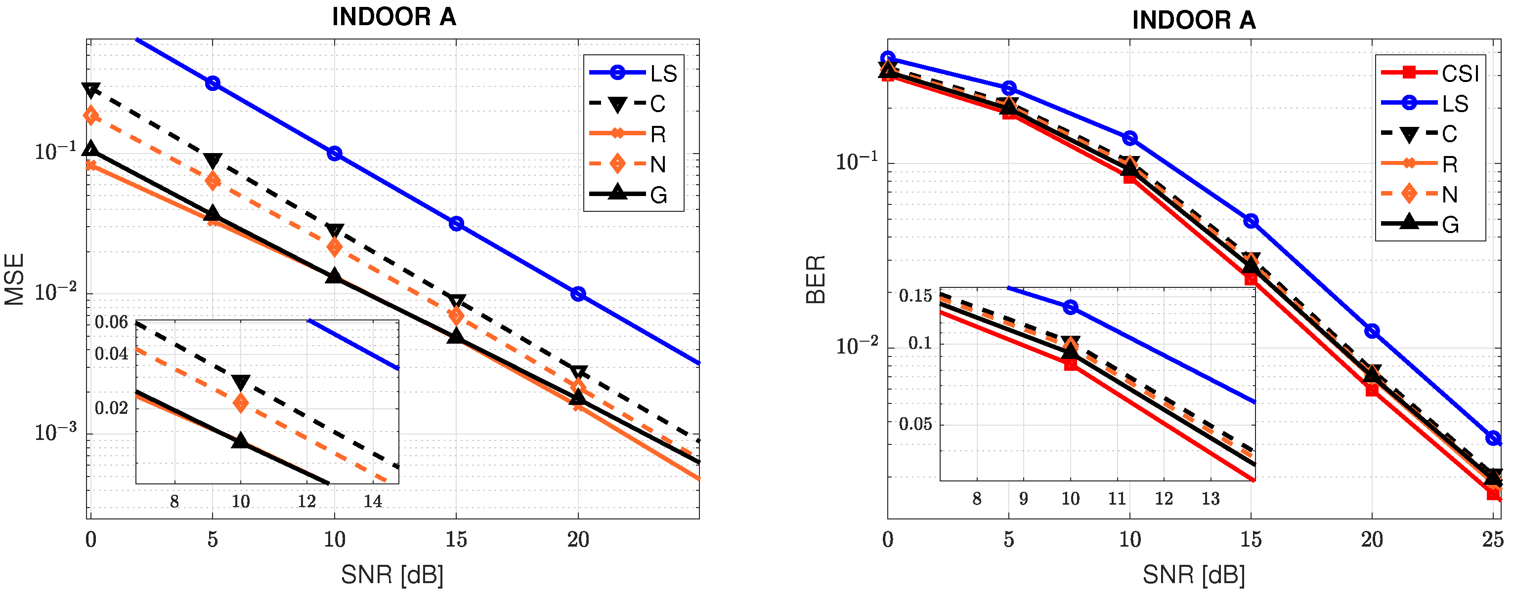
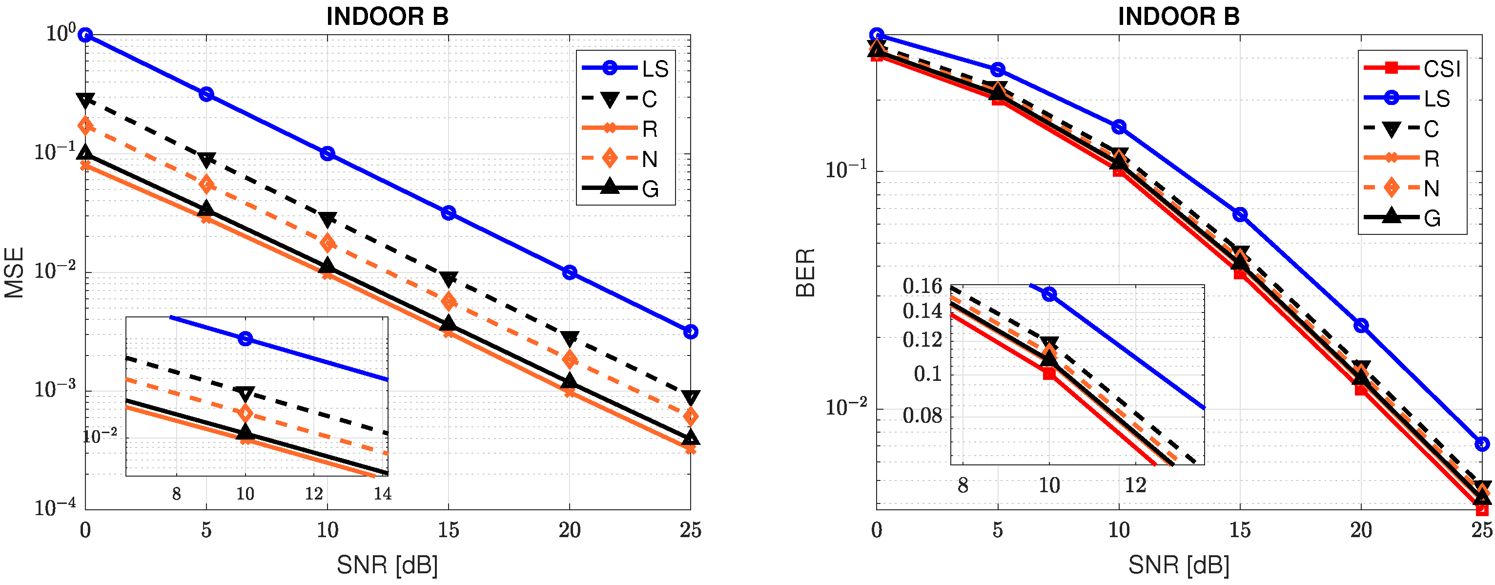
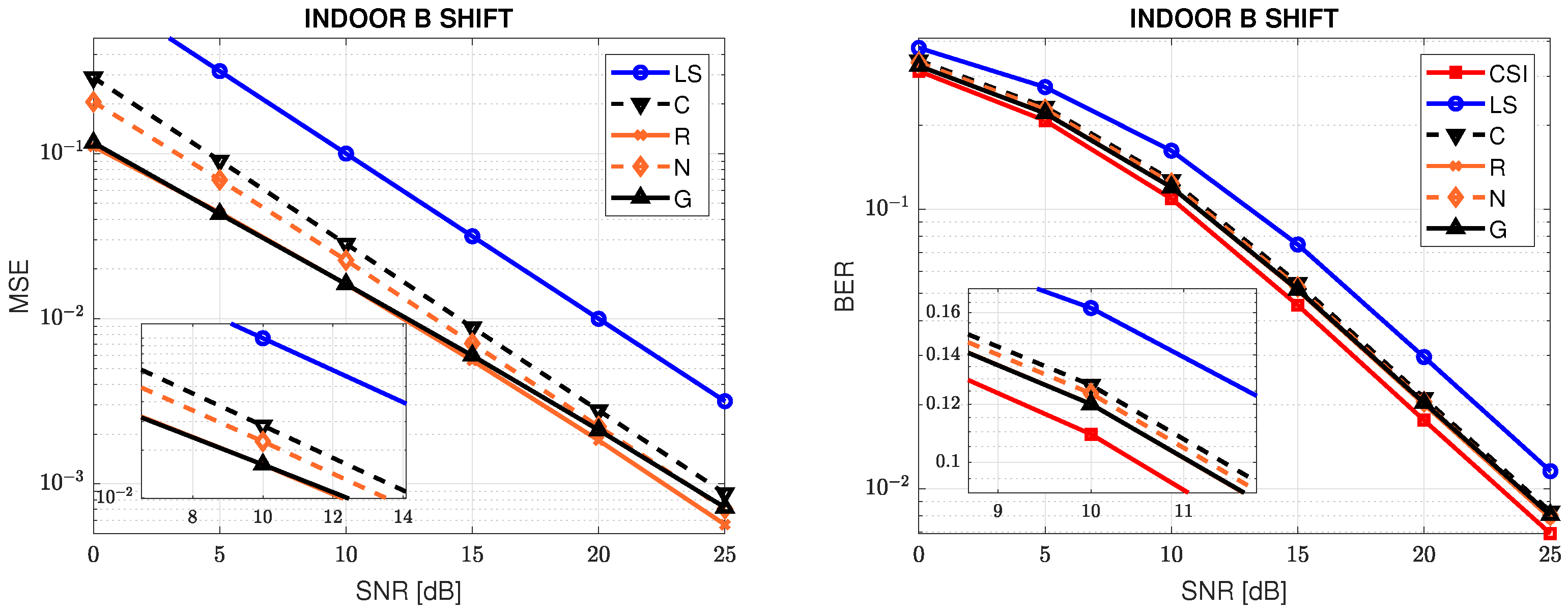
- CSI
- —full CSI available;
- LS
- —classic LS estimation method [7];
- C
- —the basic DFT-based method. The LS impulse response limited to M samples [9];
- N
- —noise energy-controlled DFT-based method with individual assignment of impulse response coefficients [14];
- R
- —residual error-controlled DFT-based method with impulse response reconstruction in groups (the authors’ modification proposed in [13]);
- G
- —the modification proposed in this article.
4.2. Results and Discussion
5. Computational Complexity Issues
- C1
- LS estimate of the frequency characteristics. It requires N complex multiplications;
- C2
- CIR calculation using N-point IFFT. The complexity is proportional to ;
- C3
- Initial selection of M consecutive CIR coefficients according to energy maximization rule. real number multiplications and N additions for the coefficients energy calculation, and additions and comparisons for the final coefficients selection are required;
- C4
- Noise power estimation according to (14) ( real number additions);
- S1
- Coefficients sorting. The coefficients of are sorted in terms of their energy. The maximum time complexity depends on implemented sorting methods and varies from to [25];
- S2
- Length U of the moving average filter. This step is performed iteratively until inequality (27) is met. Every iteration consumes a single addition and comparison. The number of iterations is proportional to SNR and corresponds to the length U.
- S3
- Fine coefficients selection out of M-element set. This processing step implements (21). additions, and the comparisons are required.
6. Conclusions
Author Contributions
Funding
Acknowledgments
Conflicts of Interest
Abbreviations
| AWGN | Additive White Gaussian Noise |
| BER | Bit Error Rate |
| CIR | Channel Impulse Response |
| CP | Cyclic Prefix |
| CS | Compressed Sensing |
| CSI | Channel State Information |
| DFT | Discrete Fourier Transform |
| FFT | Fast Fourier Transform |
| IoT | Internet of Things |
| ISI | Intersymbol Interferences |
| LDPC | Low-Density Parity Check |
| LMMSE | Linear Minimum Mean Square Error |
| LS | Least Squares |
| MIMO | Multiple Input Multiple Output |
| MSE | Mean Square Error |
| OFDM | Orthogonal Frequency Division Multiplexing |
| OMP | Orthogonal Matching Pursuit |
| QAM | Quadrature Amplitude Modulation |
| QPSK | Quadrature Phase Shift Keying |
| SNR | Singnal-Noise Ratio |
| ZF | Zero Forcing |
Appendix A
References
- Wang, Z.; Giannakis, G. Wireless multicarrier communications. IEEE Signal Process. Mag. 2000, 17, 29–48. [Google Scholar] [CrossRef]
- Liu, Y.; Tan, Z.; Hu, H.; Cimini, L.; Li, G. Channel Estimation for OFDM. IEEE Commun. Surv. Tutor. 2014, 16, 1891–1908. [Google Scholar] [CrossRef]
- Ozdemir, M.; Arslan, H. Channel estimation for wireless ofdm systems. IEEE Commun. Surv. Tutor. 2007, 9, 18–48. [Google Scholar] [CrossRef]
- Salvo Rossi, P.; Romano, G.; Ciuonzo, D.; Palmieri, F. Gain design and power allocation for overloaded MIMO-OFDM systems with channel state information and iterative multiuser detection. In Proceedings of the 2011 8th International Symposium on Wireless Communication Systems, Aachen, Germany, 6–9 November 2011; pp. 769–773. [Google Scholar] [CrossRef]
- Choi, J.Y.; Jo, H.S.; Mun, C.; Yook, J.G. Preamble-Based Adaptive Channel Estimation for IEEE 802.11p. Sensors 2019, 19, 2971. [Google Scholar] [CrossRef] [PubMed] [Green Version]
- Wang, T.; Hussain, A.; Cao, Y.; Gulomjon, S. An Improved Channel Estimation Technique for IEEE 802.11p Standard in Vehicular Communications. Sensors 2019, 19, 98. [Google Scholar] [CrossRef] [PubMed] [Green Version]
- Coleri, S.; Ergen, M.; Puri, A.; Bahai, A. Channel estimation techniques based on pilot arrangement in OFDM systems. IEEE Trans. Broadcast. 2002, 48, 223–229. [Google Scholar] [CrossRef] [Green Version]
- Savaux, V.; Louët, Y. LMMSE channel estimation in OFDM context: A review. IET Signal Process. 2017, 11, 123–134. [Google Scholar] [CrossRef]
- Edfors, O.; Sandell, M.; van de Beek, J.J.; Wilson, S.K.; Börjesson, P.O. Analysis of DFT-Based Channel Estimators for OFDM. Wirel. Pers. Commun. 2000, 12, 55–70. [Google Scholar] [CrossRef]
- Failli, M. Digital Land Mobile Radio Communications COST 207; Technical Report; Publications Office European Communities: Brussels, Luxembourg, 1989. [Google Scholar]
- Wan, L.; Qiang, X.; Ma, L.; Song, Q.; Qiao, G. Accurate and Efficient Path Delay Estimation in OMP Based Sparse Channel Estimation for OFDM With Equispaced Pilots. IEEE Wirel. Commun. Lett. 2019, 8, 117–120. [Google Scholar] [CrossRef]
- Crespo Marques, E.; Maciel, N.; Naviner, L.; Cai, H.; Yang, J. A Review of Sparse Recovery Algorithms. IEEE Access 2019, 7, 1300–1322. [Google Scholar] [CrossRef]
- Dziwoki, G.; Kucharczyk, M.; Izydorczyk, J. Modified OMP Algorithm for Compressible Channel Impulse Response Estimation. In Computer Networks; Gaj, P., Sawicki, M., Suchacka, G., Kwiecień, A., Eds.; Springer International Publishing: Cham, Switzerland, 2018; pp. 161–170. [Google Scholar]
- Kang, Y.; Kim, K.; Park, H. Efficient DFT-based channel estimation for OFDM systems on multipath channels. IET Commun. 2007, 1, 197–202. [Google Scholar] [CrossRef]
- Gu, F.; Fan, Y.; Wang, L.; Tan, X.; Wei, J. A Universal Channel Estimation Algorithm Based on DFT Smoothing Filtering. IEEE Access 2019, 7, 129883–129891. [Google Scholar] [CrossRef]
- Dziwoki, G.; Kucharczyk, M. On a sparse approximation of compressible signals. Circuits Syst. Signal Process. 2020, 39, 2232–2243. [Google Scholar] [CrossRef] [Green Version]
- Sułek, W. Non-binary LDPC Decoders Design for Maximizing Throughput of an FPGA Implementation. Circuits Syst. Signal Process. 2016, 35, 4060–4080. [Google Scholar] [CrossRef]
- Sułek, W. Protograph Based Low-Density Parity-Check Codes Design With Mixed Integer Linear Programming. IEEE Access 2019, 7, 1424–1438. [Google Scholar] [CrossRef]
- Watanabe, K.; Higuchi, S.; Maruta, K.; Ahn, C.J. Performance of polar codes with MIMO-OFDM under frequency selective fading channel. In Proceedings of the 2017 20th International Symposium on Wireless Personal Multimedia Communications (WPMC), Bali, Indonesia, 17–20 December 2017; pp. 107–111. [Google Scholar] [CrossRef]
- Guidelines for Evaluation of Radio Transmission Technologies for IMT-2000; Technical Report Rec.ITU-R M.1225; International Telecommunication Union: Geneva, Switzerland, 1997.
- Tropp, J.; Gilbert, A. Signal Recovery From Random Measurements Via Orthogonal Matching Pursuit. IEEE Trans. Inf. Theory 2007, 53, 4655–4666. [Google Scholar] [CrossRef] [Green Version]
- Haykin, S.O. Adaptive Filter Theory; Prentice Hall: Bergen, NJ, USA, 1996. [Google Scholar]
- Rappaport, T.S. Wireless Communications: Principles and Practice; Prentice Hall: Bergen, NJ, USA, 2002. [Google Scholar]
- Zhong, Z.; Fan, L.; Ge, S. FDD Massive MIMO Uplink and Downlink Channel Reciprocity Properties: Full or Partial Reciprocity? In Proceedings of the GLOBECOM 2020-2020 IEEE Global Communications Conference, Taipei, Taiwan, 7–11 December 2020; pp. 1–5. [Google Scholar] [CrossRef]
- Cormen, T.H.; Leiserson, C.E.; Rivest, R.L.; Stein, C. Introduction to Algorithms; The MIT Press: Cambridge, MA, USA, 2009. [Google Scholar]
- Dey, I.; Ciuonzo, D.; Rossi, P.S. Wideband Collaborative Spectrum Sensing Using Massive MIMO Decision Fusion. IEEE Trans. Wirel. Commun. 2020, 19, 5246–5260. [Google Scholar] [CrossRef]


| CIR Estimation Method | Single/In groups CIR Coefficients Reconstruction Approach | Noise/Residual Energy Based Error Metric |
|---|---|---|
| Classical DFT-based [9] | −/+ | −/− |
| Modified DFT-based [14,15] | +/− | +/− |
| Classical CS [12] | +/− | −/+ |
| Block CS [13] | −/+ | −/+ |
| Proposed | –/+ | +/– |
| Parameter | Value |
|---|---|
| Carrier frequency | = 2 GHz |
| Sampling frequency | = 10 MHz |
| Active subchannels | N = 128 |
| FFT size | N = 128 |
| Cyclic prefix length | M = 32 (samples) |
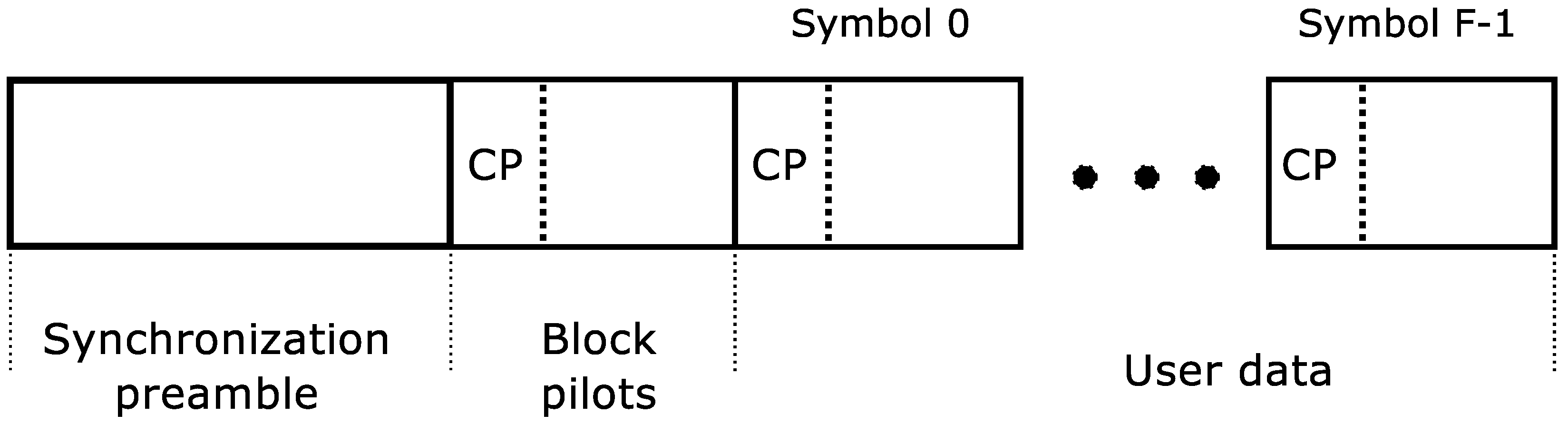
| Synchronization sequence | P = 256 (samples) |
| Synchronization factor | |
| Block-pilot OFDM symbols per frame | 1 |
| Pilot constellation | QPSK |
| Data OFDM symbols per frame | F = 50 |
| Frame duration | μs |
| Data constellation | 16-QAM, 64-QAM |
| Data frames per transmission | 50 |
| Maximum speed | v = 10 km/h |
| Doppler spread | Hz |
| Coherence time [23] | ms |
| SNR range | dB with 5 dB step |
| Channel | Average Relative Paths Delays [ns] | Average Paths Gains [dB] |
|---|---|---|
| Indoor A [20] | [0, 50, 110, 170, 290, 310] | [0, −3, −10, −18, −26, −32] |
| Indoor B [20] | [0, 100, 200, 300, 500, 700] | [0, −3.6, −7.2, −10.8, −18, −25.2] |
| Indoor B Shift | [50, 150, 250, 350, 450, 750] | [0, −3.6, −7.2, −10.8, −18, −25.2] |
| Outdoor-To-Indoor A [20] | [0, 110, 190, 410] | [0, −9.7, −19.2, −22.8] |
| BER | Indoor A | Indoor B | Indoor B Shift | Outdoor-to-Indoor A |
|---|---|---|---|---|
| 0.1 | 0.3 dB | 0.2 dB | 0.2 dB | 0.3 dB |
| 0.01 | 0.1 dB | 0.2 dB | 0 dB | 0.2 dB |
| SNR | Indoor A | Indoor B | Indoor B Shift | Outdoor-to-Indoor A |
|---|---|---|---|---|
| 0 dB | 5 | 5 | 7 | 4 |
| 5 dB | 6 | 5 | 9 | 4 |
| 10 dB | 8 | 6 | 11 | 5 |
| 15 dB | 11 | 7 | 14 | 6 |
| 20 dB | 14 | 7 | 15 | 7 |
| 25 dB | 15 | 8 | 17 | 8 |
| BER | Indoor A | Indoor B | Indoor B Shift | Outdoor-to-Indoor A |
|---|---|---|---|---|
| 0.1 | 0 dB | 0.05 dB | 0.01 dB | 0.1 dB |
| 0.01 | 0.04 dB | 0.07 dB | 0.11 dB | 0.05 dB |
Publisher’s Note: MDPI stays neutral with regard to jurisdictional claims in published maps and institutional affiliations. |
© 2021 by the authors. Licensee MDPI, Basel, Switzerland. This article is an open access article distributed under the terms and conditions of the Creative Commons Attribution (CC BY) license (https://creativecommons.org/licenses/by/4.0/).
Share and Cite
Dziwoki, G.; Kucharczyk, M. Estimation of Compressible Channel Impulse Response for OFDM Modulated Transmissions. Electronics 2021, 10, 2781. https://doi.org/10.3390/electronics10222781
Dziwoki G, Kucharczyk M. Estimation of Compressible Channel Impulse Response for OFDM Modulated Transmissions. Electronics. 2021; 10(22):2781. https://doi.org/10.3390/electronics10222781
Chicago/Turabian StyleDziwoki, Grzegorz, and Marcin Kucharczyk. 2021. "Estimation of Compressible Channel Impulse Response for OFDM Modulated Transmissions" Electronics 10, no. 22: 2781. https://doi.org/10.3390/electronics10222781
APA StyleDziwoki, G., & Kucharczyk, M. (2021). Estimation of Compressible Channel Impulse Response for OFDM Modulated Transmissions. Electronics, 10(22), 2781. https://doi.org/10.3390/electronics10222781