TRIG: Transformer-Based Text Recognizer with Initial Embedding Guidance

Abstract

Scene text recognition (STR) is an important bridge between images and text, attracting abundant research attention. While convolutional neural networks (CNNS) have achieved remarkable progress in this task, most of the existing works need an extra module (context modeling module) to help CNN to capture global dependencies to solve the inductive bias and strengthen the relationship between text features. Recently, the transformer has been proposed as a promising network for global context modeling by self-attention mechanism, but one of the main short-comings, when applied to recognition, is the efficiency. We propose a 1-D split to address the challenges of complexity and replace the CNN with the transformer encoder to reduce the need for a context modeling module. Furthermore, recent methods use a frozen initial embedding to guide the decoder to decode the features to text, leading to a loss of accuracy. We propose to use a learnable initial embedding learned from the transformer encoder to make it adaptive to different input images. Above all, we introduce a novel architecture for text recognition, named TRansformer-based text recognizer with Initial embedding Guidance (TRIG), composed of three stages (transformation, feature extraction, and prediction). Extensive experiments show that our approach can achieve state-of-the-art on text recognition benchmarks.

1. Introduction

STR, aiming to read the text in natural scenes, is an important and active research field in computer vision [1,2]. Text reading can obtain semantic information from images, playing a significant role in a variety of vision tasks, such as image retrieval, key information extraction, and document visual question answering.

Among the feature extraction module of existing text recognizers, convolutional architectures remain dominant. For example, ASTER [3] uses ResNet [4] and SRN [5] uses FPN [6] to aggregate hierarchical feature maps from ResNet50. As we all know, the text has linguistic information and almost every character has a relationship with each other. So features with global contextual information can decode more accurate characters. Unfortunately, the convolutional neural network has an inductive bias on locality for the design of the kernel. It lacks the ability to model long-range dependencies, hence text recognizers should use context modeling structures to gain better performance. It is a common practice that Bi-directional LSTM (BiLSTM) [7] is effective to enhance context modeling. Such context modeling modules introduce additional complexity and operations. So a question comes: Why not replace CNN with another network which can model long-range dependencies in a feature extractor without an additional context modeling module?

With the introduction of the transformer [8], the question has an answer. Recently, it has been proposed to regard an image as a sequence of patches and aggregate feature in global context by self-attention mechanisms [9]. Therefore, we propose to use a pure transformer encoder as the feature extractor instead of CNN. Due to the ability of dynamic attention, global context, and better generalization of the transformer, the transformer encoder can provide global and robust features without the extra context modeling module. By this way, we can simplify the four-stage STR framework (transformation stage, feature extraction stage, context modeling stage, and prediction stage) proposed in Baek et al. [10] to three stages by removing the need for a context modeling module. Our extensive experiments prove the effectiveness of the three-stage architecture. It shows that the additional context modeling module degrades performance rather than any gain and the feature extractor exactly models long-range dependencies when using the transformer encoder.

Despite the strong ability of the transformer, the high demand for memory and computation resources may cause difficulty in the training and inference process. For example, the authors of Vision Transformer (ViT) [9] used extensive computing resources to train their model (about 230 TPUv3-core-days for the ViT-L/16). It is hard for researchers to access such huge resources. The main reason for the high complexity of the transformer is the self-attention mechanism inside. Complexity and sequence length are squared. Therefore, reducing the sequence length can effectively reduce the complexity. With the consideration of efficiency, we do not simply use the square patch size proposed in the ViT-like backbone used in image classification, segmentation, and object detection [11,12,13,14]. Instead, we propose the 1-D split to split the picture into rectangle patches whose height is the same as the input image, shown in Figure 1c. In this way, the image can convert to a sequence of patches (1-D split) whose length is shorter than the 2-D split (the height of patch size is smaller than the input image). The design of patch size has the advantage of fewer Multiply Accumulate operations (MACs), which leads to faster training and inference with fewer resources.

The prediction stage is another important part of the text recognizer, which decodes the feature to text. An attention-based sequence decoder is commonly used in previous works and has a hidden state embedding to guide the decoder. Recent methods [3,15,16] use the frozen zero embedding to initialize the hidden state, which remains the same when different images are inputted, influencing the accuracy of the decoder. To make the hidden state of the decoder adaptive to different inputs, we propose a learnable initial embedding learned from the transformer encoder to dynamically learn information from images. The adaptive initial embedding can guide the decoding process to reach better accuracy.

To sum up, this paper presents three main contributions:

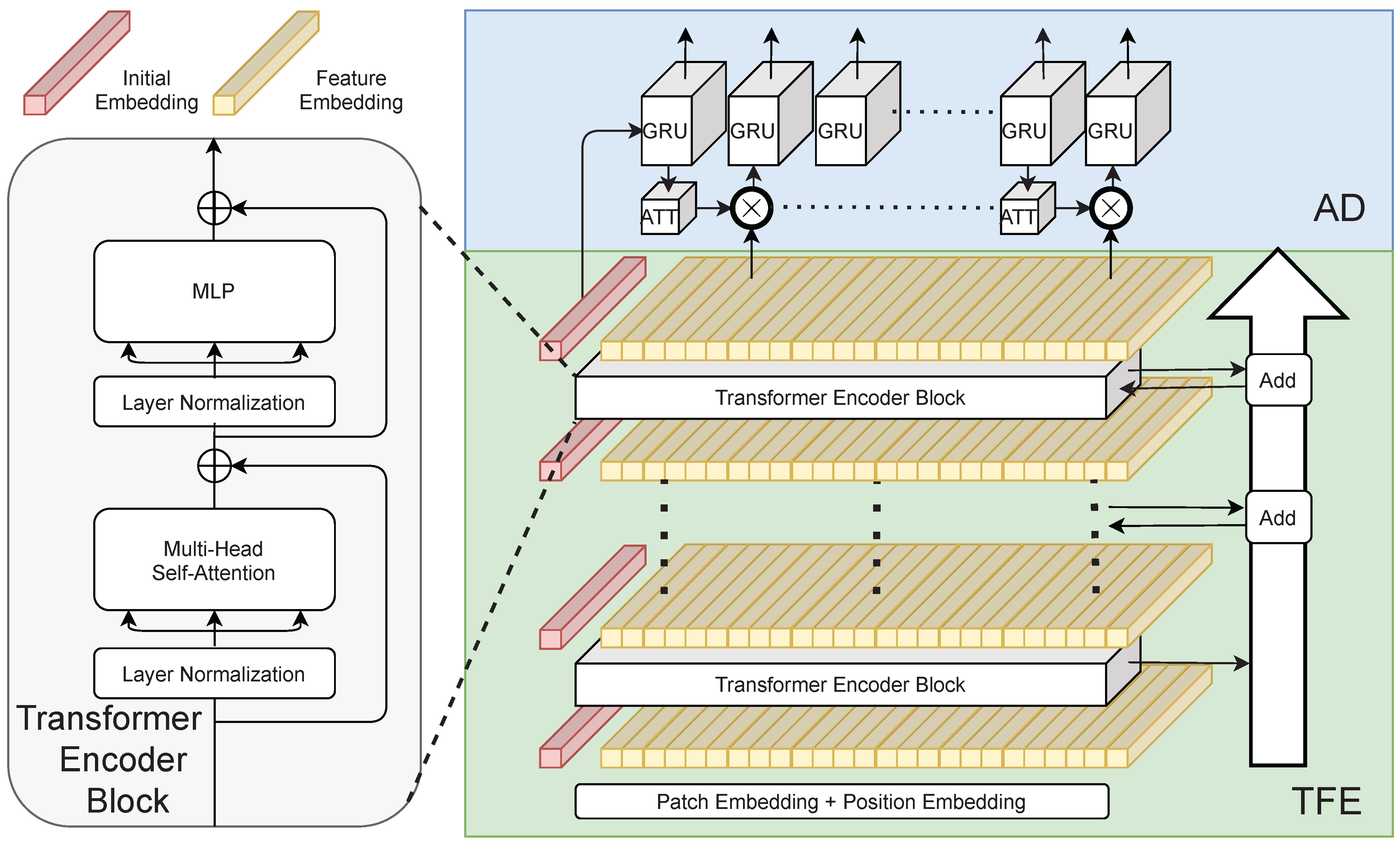
• We propose a novel three-stage architecture for text recognition, TRIG, namely Transformer-based text recognizer with Initial embedding Guidance. TRIG leverages the transformer encoder to extract global context features without an additional context modeling module used in CNN-based text recognizers. Extensive experiments on several public scene text benchmarks demonstrate the proposed framework can achieve state-of-the-art (SOTA) performance.
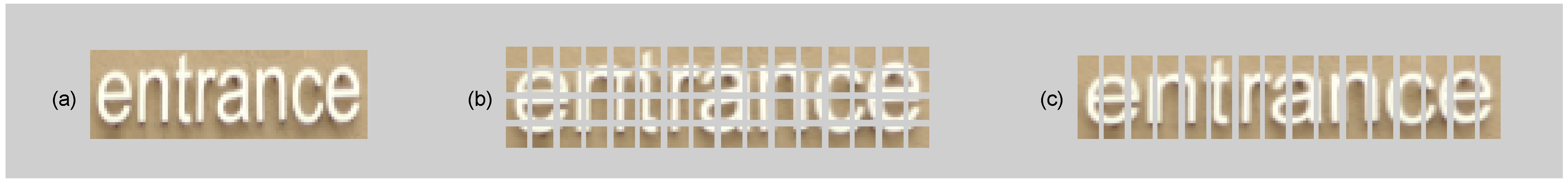
• A 1-D split is designed to divide the text image as a sequence of rectangle patches with the consideration of efficiency.
• We propose a learnable initial embedding to dynamically learn information from the whole image, which can be adaptive to different input images and precisely guide the decoding process.

2. Related Work

Most traditional scene text recognition methods [17,18,19,20,21] adopt a bottom-up approach, which first detects individual characters with a sliding window and classifies them by using hand-crafted features. With the development of deep learning, top-down methods were proposed. These approaches can be roughly divided into two categories by applying a transformer or not, namely transformer-free methods and transformer-based methods.

2.1. Transformer-Free Methods

Before the proposal of the transformer, STR methods only use CNN and recurrent neural network (RNN) to read the text. CRNN [22] extracts feature sequences using CNN, and then encodes the sequence by RNN. Finally, Connectionist Temporal Classification (CTC) [23] decodes the sequence to the text results. By design, this method is hard to address curve or rotated text. To deal with it, Aster proposes the method of spatial transformer networks (STN) [24] with the 1-D attention decoder. Without spatial transformation [15,25], propose methods to handle irregular text recognition by 2-D CTC decoder or 2-D attention decoder. Furthermore, segmentation-based methods [26] can also be used to read text, which should be supervised by character-level annotations. SEED [27] uses semantic information which is supervised by a pre-trained language model to guide the attention decoder.

2.2. Transformer-Based Methods

The transformer, first applied to the field of machine translation and natural language processing, is a type of neural network mainly based on the self-attention mechanism. Inspired by NLP success, ViT applies a pure transformer to tackle the image classification tasks and attains comparable results. Then, Data-efficient Image Transformers (DeiT) [11] achieves competitive accuracy with no external data. Unlike ViT and DeiT, the detection transformer (DETR) [28] uses both the encoder and decoder parts of the transformer. DETR is a new framework of end-to-end detectors, which attains comparable accuracy and inference speed with Faster R-CNN [29].

We summarize four ways to use a transformer in STR. (a) Master [16] uses the decoder of the transformer to predict output sequence. It owns a better training efficiency. In the training stage, a transformer decoder can predict out all-time steps simultaneously by constructing a triangular mask matrix. (b) a transformer can be used to translate from one language to another. So SATRN [30] and NRTR [31] adopt the encoder-decoder of the transformer to address the cross-modality between the image input and text output. The image input represents features extracted by shallow CNN. In addition, SATRN proposes two new changes in the transformer encoder. It uses an adaptive 2D position encoding and adds convolution in feedforward layer. (c) SRN [5] not only adopts the transformer encoder to model context but also uses it to reason semantic. (d) the transformer encoder works as a feature extractor including context modeling. Our work uses this method of using the transformer encoder. It is different from recent methods.

3. Methodology

This section describes our three-stage text recognition model, TRIG, in full detail. As shown in Figure 2, our approach TRIG consists of three stages: Transformation, Transformer feature extractor, and attention decoder. TRA rectifies the input text by a thin-plate spline (TPS) [32]. TFE provides robust visual features. AD decodes the feature map to characters. First, we describe the stage of TRA. Second, we show the details of the stage of TFE. Then, the AD stage is presented. After that, we introduce the loss function. Finally, we analyze the efficiency of our method with different patch sizes.

3.1. Transformation

Transformation is a stage to rectify the input text images by rectification module. This module uses a shallow CNN to predict several control points, and then TPS transformation is applied to diverse aspect ratios of text lines. In this way, the perspective and curve text can be rectified. Note, the picture becomes the size of $32\times 100$ here.

3.2. Transformer Feature Extractor

The TFE is illustrated in Figure 3. In this stage, the transformer encoder is used to extract effective and robust features. First, the rectified image is split into patches. Unlike the square size of patches in [9,11,12,13,14], the rectified image is split into rectangle patches, whose size is $h\times w$ (h is same as the height of the rectified image). Then the rectified image $X\in {\mathbb{R}}^{H\times W\times C}$, where $H,W,C$ is the height, width, and channel of the rectified image, can be mapped to a sequence $X_s\in {\mathbb{R}}^{(H\times W÷(h\times w\left)\right)\times (3\times h\times w)}$. Then, a trainable linear projection $W_E$$\in {\mathbb{R}}^{(3\times h\times w)\times D}$ (embedding matrix) is used to obtain the patch embeddings $E\in {\mathbb{R}}^{(H\times W÷(h\times w\left)\right)\times D}$, where D is the dimension of patch embeddings. The transcription procedure is given by:

$$E=X_s{W}_E$$

(1)

In our implementation, we use a patch size of $32\times 4$ and thus the feature dimension of patch sequence is $32\times 4\times 3=384$. The size of the rectified image is $32\times 100$, so the length of patch sequence is $(32\times 100)÷(32\times 4)=25$. After that the patch sequence is projected using a linear mapping function with a projection matrix $W_E\in {\mathbb{R}}^{384\times 512}$, resulting in the patch embeddings $E\in {\mathbb{R}}^{25\times 512}$.

Initial embedding $E_{init}$ is a trainable vector, appended to the sequence of patch embeddings, which goes through transformer encoder blocks, and is then used to guide the attention decoder. Similar to the role of class token in ViT, we introduce a trainable vector $E_{init}$ called Initial embedding. In order to encode the position information of each patch embeddings, we use the standard learnable position embeddings. The position embedding can be parameterized by a learnable positional embedding table. For example, position i has i-th position embedding in the embedding table. The position embeddings $E_{pos}$ have the same dimension D as patch embeddings. At last, the input feature embeddings $F_0$$\in {\mathbb{R}}^{(H\times W÷(h\times w)+1)\times D}$ is the sum of position embeddings and patch embeddings:

$$F_0=concat(E_{init},E)+E_{pos}$$

(2)

Transformer encoder blocks are applied to the obtained input feature embeddings $F_0$. As we all know, the transformer encoder block consists of multi-head self-attention (MSA) and multi-layer perceptron (MLP). Following the architecture from ViT, layer normalization (LN) is applied before MSA and MLP. The MLP contains two linear transformations layers with a GELU non-linearity. The dimension of input and output is the same, and the dimension of the inner-layer is four times the output dimension. The transformer encoder block can be represented as following equations:

$$\begin{array}{ccc}\hfill F_l^{{}^{\prime }}=MSA\left(LN\left(F_{l-1}\right)\right)+F_{l-1},& \hfill & \hfill l=1,2\dots L\end{array}$$

(3)

$$\begin{array}{ccc}\hfill F_l=MLP\left(LN\left(F_l^{{}^{\prime }}\right)\right)+F_l^{{}^{\prime }},& \hfill & \hfill l=1,2\dots L\end{array}$$

(4)

where l denotes the index of blocks, and L is the index of the last block. The dimension of $F_l$ and $F_l^{{}^{\prime }}$ is D and $4D$.

To obtain better performance, we add a Residual add module. The Residual add module uses skip edge to connect MSA modules in adjacent blocks, following Realformer [33]. The multi-head process can be unified as:

$$\begin{array}{c}\hfill MultiHead(Q,K,V,P)=Concat(hea{d}_1,\dots hea{d}_h)W^O\\ \hfill hea{d}_i=Attention(Q{W}_i^Q,K{W}_i^K,V{W}_i^V,P)\end{array}$$

(5)

$$\begin{array}{c}\hfill =Softmax(\frac{Q{W}_i^Q{\left(K{W}_i^K\right)}^T}{\sqrt{d_k}}+P)V{W}_i^V.\end{array}$$

(6)

where query matrix Q, key matrix K and value matrix V are linearly projected by $W_i^Q$, $W_i^K$, $W_i^V$. P is the previous attention score $\frac{Q{W}_i^Q{\left(K{W}_i^K\right)}^T}{\sqrt{d_k}}+P^{{}^{\prime }}$ in the previous block.

After transformer feature extraction, the feature map $F_L=[f_{init},f_1,f_2,\dots f_N]$ can be obtained. Please note that f means feature embedding. N denotes the index of feature embeddings without $f_{init}$.

3.3. Attention Decoder

The architecture is illustrated in Figure 3. We use an attention decoder to decode the sequence of the feature map. $f_{init}$ is used to initialize the RNN decoder and $[f_1,f_2,\dots ,f_N]$ is used as the input of the decoder. First, we obtain an attention map from the feature map and the internal state from RNN:

$$\begin{array}{c}\hfill e_{t,i}=w^{T}tanh(W_d{s}_{t-1}+V_d{f}_i+b)\end{array}$$

(7)

$$\begin{array}{c}\hfill {\alpha }_{t,i}=\frac{exp\left(e_{t,i}\right)}{{\sum }_{i^{{}^{\prime }}=1}^n{e}_{t,i^{\prime }}}\end{array}$$

(8)

where $b,w,W_d,V_d$ are trainable parameters, $s_{t-1}$ is the hidden state of the recurrent cell within the decoder at time t. Specifically, $s_0$ is equivalent to $f_{\mathit{init}}$.

Then, we use attention map to element-wise product the feature map $[f_1,f_2,\dots ,f_N]$, and combine all of them to obtain a vector $g_t$ which called a glimpse:

$$\begin{array}{c}\hfill g_t=\sum _{i=1}^n{\alpha }_{t,i}{f}_i\end{array}$$

(9)

Next, RNN is used to produce an output vector and a new state vector. The recurrent cell of the decoder is fed with:

$$\begin{array}{c}\hfill (x_t,s_t)=RNN(s_{t-1},[g_t,f\left(y_{t-1}\right)]),\end{array}$$

(10)

where $[g_t,f\left(y_{t-1}\right)]$ denotes the concatenation between $g_t$ and the one-hot embedding of $y_{t-1}$.

Here, we use GRU [34] as our recurrent unit. At last, the probability for a given character can be expressed as:

$$\begin{array}{c}\hfill p\left(y_t\right)=softmax(W_0{x}_t+b_o).\end{array}$$

(11)

3.4. Training Loss

Here, we use the standard cross-entropy loss, which can be defined as:

$$\begin{array}{c}\hfill L_{CE}=-\sum _{t=1}^T\left(logp\left(y_t\right|I)\right),\end{array}$$

(12)

where $y_1,y_2,\dots ,y_T$ is the groundtruth text represented by a character sequence.

3.5. Efficiency Analysis

For the TFE, we assume that the hidden dimension of the TFE is D and that the input sequence length is T. The complexity of self-attention and MLP is $O(T^2\times D)$ and $O(T\times D^2)$. Comparing the 1-D split (rectangle patch with the size of 32 × 4) with the 2-D split (square patch with the size of 4 × 4), the sequence lengths are, respectively, 26 and 201, when the input image is 32 × 100. As ${201}^2\gg {26}^2$ and $201>26$, the complexity and MACs of the 2-D split are far more than the 1-D split. The MACs of TFE are, respectively, 1.641 G and 12.651 G, when using 1-D split and 2-D split.

For the decoder, the complexity gap between 1 and D split and 2-D split comes from the process of obtaining an attention map and glimpse. We assume that the sequence length is T. The complexities are both $O\left(T\right)$. Therefore, the shorter sequence has lower complexity. The MACs of AD using the 1-D split is 0.925 G when it is 5.521 G using the 2-D split.

Based on the above analysis, we propose to use a 1-D split to increase efficiency.

4. Experiments

In this section, we demonstrate the effectiveness of our proposed method. First, we give a brief introduction to the datasets and the implementation details. Then, our method is compared with state-of-the-art methods on several public benchmark datasets. Next, we make some discussions on our method. Finally, we perform ablation studies to analyze the performance of different settings.

4.1. Dataset

In this paper, models are only trained on two public synthetic datasets MJSynth (MJ) [35] and SynText (ST) [36] without any additional synthetic dataset, real dataset or data augmentation. There are 7 scene text benchmarks chosen to evaluate our models.

MJ contains 9 million word box images, which is generated from a lexicon of 90 K English words.

ST is a synthetic text dataset generate by an engine proposed in [36]. We obtain 7 million text lines from this dataset for training.

IIIT5K (IIIT) [37] contains scene texts and born-digital images, which are collected from the website. It consists of 3000 images for evaluation.

Street View Text (SVT) [38] is collected from the Google Street View. It contains 647 images for evaluation, some of which are severely corrupted by noise and blur or have low resolution.

ICDAR 2003 (IC03) [39] have two different versions of the dataset for evaluation: versions with 860 or 867 images. We use 867 images for evaluation.

ICDAR 2013 (IC13) [40] contains 1015 images for evaluation.

ICDAR 2015 (IC15) [41] contains 2077 images, captured by Google Glasses, some of which are noisy, blurry, and rotated or have low resolution. Researchers have used two different versions for evaluation: 1811 and 2077 images. We use both of them.

SVT-Perspective (SVTP) [21] contains 645 cropped images for evaluation. Many of the images contain perspective projections due to the prevalence of non-frontal viewpoints.

CUTE80 (CUTE) [42] contains 288 cropped images for evaluation. Many of these are curved text images.

4.2. Implementation Details

The proposed TRIG is implemented in the PyTorch framework and trained on two RTX2080Ti GPUs with 11 GB memory. As for the training details, we do not perform any type of pre-training. The decoder recognizes 97 character classes, including digits, upper-case and lower-case letters, 32 ASCII punctuation marks, end-of-sequence (eos) symbol, padding symbol, and unknown symbol. We adopt the AdaDelta optimizer and the decayed learning rate. Our model is trained on ST and MJ for 24 epochs with a batch size of 640, the learning rate is set to 1.0 initially and decayed to 0.1 and 0.01 at the 19th and the 23rd epoch. The batch is sampled 50% from ST and 50% from MJ. All images are resized to $64\times 256$ during both training and testing. We use the IIIT dataset to select our best model.

At inference, we resize the images to the same size as for training. Furthermore, we use beam search by maintaining five candidates with the top accumulative scores at every step to decode.

4.3. Comparison with State-of-the-Art

We compare our methods with previous state-of-the-art methods on several benchmarks. The results are shown in

Table 1. Comparison with SOTA methods. ’SA’, ’R’ indicates using SynthAdd dataset or real datasets apart from MJ and ST. ’A’ means using data augmentation when training. For a fair comparison, reported results using additional data or data augmentation are not taken into account. Top accuracy for each benchmark is shown in bold. The average accuracy is calculated on seven datasets and IC15 using the version which contains 2077 images.

Method	Training Data	IIIT 3000	SVT 647	IC03 867	IC13 1015	IC15 1811	IC15 2077	SVTP 645	CUTE 288	Average
CRNN [22]	MJ	78.2	80.8	-	86.7	-	-	-	-	-
FAN [43]	MJ + ST	87.4	85.9	94.2	93.3	-	70.6	-	-	-
ASTER [3]	MJ + ST	93.4	89.5	94.5	91.8	76.1	-	78.5	79.5	-
SAR [15]	MJ + ST	91.5	84.5	-	91.0	-	69.2	76.4	83.3	-
ESIR [44]	MJ + ST	93.3	90.2	-	91.3	76.9	-	79.6	83.3	-
MORAN [45]	MJ + ST	91.2	88.3	95.0	92.4	-	68.8	76.1	77.4	84.5
SATRN [30]	MJ + ST	92.8	91.3	96.7	94.1	-	79	86.5	87.8	89.2
DAN [46]	MJ + ST	94.3	89.2	95.0	93.9	-	74.5	80.0	84.4	87.7
RobustScanner [47]	MJ + ST	95.3	88.1	-	94.8	-	77.1	79.2	90.3	-
PlugNet [48]	MJ + ST	94.4	92.3	95.7	95.0	82.2	-	84.3	85.0	-
AutoSTR [49]	MJ + ST	94.7	90.9	93.3	94.2	81.8	-	81.7	-	-
GA-SPIN [50]	MJ + ST	95.2	90.9	-	94.8	82.8	79.5	83.2	87.5	-
MASTER [16]	MJ + ST + R	95	90.6	96.4	95.3	-	79.4	84.5	87.5	90.0
GTC [51]	MJ + ST + SA	95.5	92.9	-	94.3	82.5	-	86.2	92.3	-
SCATTER [52]	MJ + ST + SA + A	93.9	90.1	96.6	94.7	-	82.8	87	87.5	90.5
RobustScanner [47]	MJ + ST + R	95.4	89.3	-	94.1	-	79.2	82.9	92.4	-
SRN [5]	MJ + ST + A	94.8	91.5	-	95.5	82.7	-	85.1	87.8	-
TRIG	MJ + ST	95.1	93.8	95.3	95.2	84.8	81.1	88.1	85.1	90.8

. Even compared to reported results using additional real or private data and data augmentation, we achieve satisfying performance. Compared with other methods trained only by MJ and ST, our method achieves the best results on four datasets including SVT, IC13, IC15, and SVTP. TRIG provides an accuracy of +1.5 percentage point (pp, 93.8% vs. 92.3%) on SVT, +0.2 pp (95.2% vs. 95.0%) on IC13, +1.6 pp (81.1% vs. 79.5%) on IC15 and +1.6 pp (88.1% vs. 86.5%) on SVTP. Here, accuracy means the success rate of word predictions. For example, 99% accuracy means that 990 out of 1000 words are correctly recognized.

4.4. Discussion

4.4.1. Discussion on Training Procedures

Our method TRIG needs long training epochs. We train TRIG and ASTER with the same learning rate and optimizer for 24 epochs. The whole training procedure takes a week. The learning rate, which is 1.0, drops by a factor of 10 after 19 and 23 epochs. As shown in Figure 4, the accuracy of TRIG on IIIT is lower than ASTER in the preceding epoch and better than ASTER after 14 epochs. At last, the accuracy of TRIG on IIIT and its average accuracy on all datasets is 0.8pp and 2pp higher than ASTER. We can conclude that the transformer feature extractor needs longer epochs to train to improve the accuracy. Because the transformer does not have properties such as CNN (i.e., shift, scale, and distortion invariance).

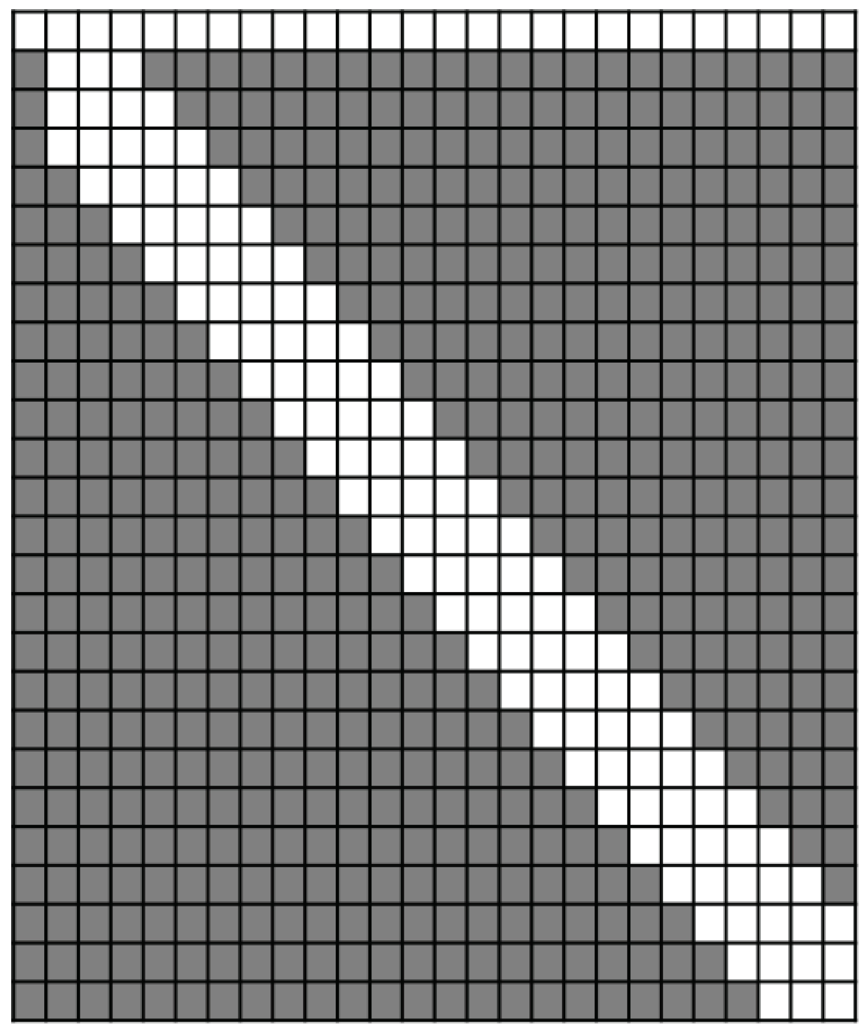
4.4.2. Discussion on Long-Range Dependencies

The decoder of the transformer uses triangle masks to promise that the prediction of one-time step t can only access the output information of its previous steps. Taking inspiration from this, we use the mask to let the transformer encoder only access the nearby feature embeddings. By this, the transformer encoder will have a small reception. We empirically analyze the performance of long-range dependencies by comparing two kinds of methods with or without masks, demonstrated in

Table 2. Performance comparison with mask and context modeling module. There are two kinds of decoder, CTC and attention decoder. All models are trained on two synthetic datasets. The batch size is 896 and the training step is 300,000. The number of blocks in TFE is 6 and skip attention is not used.

Mask	Context Modeling	Decoder	IIIT 3000	SVT 647	IC03 867	IC13 2015	IC15 2077	SVTP 645	CUTE 288
×	✓	CTC	85.0	80.4	91.7	89.6	65.8	70.5	69.4
✓	×	CTC	85.6	80.5	90.9	88.4	63.1	65.6	67.7
×	×	CTC	86.5	82.1	92.0	89.6	65.9	71.9	71.2
×	✓	Attn	87.9	86.7	92.3	90.8	71.9	79.4	72.9
✓	×	Attn	86.7	83.5	91.6	89.5	70.7	78.5	67.7
×	×	Attn	89.5	88.6	93.7	92.5	74.1	79.2	76.4

. The detail of the mask is shown in Figure 5. We observe the decrease of accuracy when using mask no matter CTC decoder and attention decoder. It indicates that long-range dependencies are related to effectiveness and the feature extractor of our method can capture long-range dependencies.

4.4.3. Discussion on Extra Context Modeling Module

As the effective module of context modeling is used in STR networks, we consider whether we need an extra context modeling module when using the transformer encoder to extract features. After the transformer feature extractor, a context modeling module (BiLSTM) is added. As shown in Table 2, the accuracy of almost all data sets is lower than methods without BiLSTM (except +0.2pp on SVTP); therefore, we conclude that it is not necessary to add BiLSTM after the transformer feature extractor to the model context, because the transformer feature extractor has an implicit ability to model context. An extra context modeling module may break the context modeling that the model has implicitly learned.

4.4.4. Discussion on Patch Size

Table 3. Performance comparison with different patch size. ’Average’ denotes the average accuracy of seven standard benchmarks. * indicates that the model did not converge, possibly because sequence length is too short to decode.

	Patch Size	Sequence Length	Average
1-D split	32 × 2	1 × 50	80.9
1-D split	32 × 4	1 × 25	83.5
1-D split	32 × 5	1 × 20	81.0
1-D split	32 × 10	1 × 10	81.7
1-D split	32 × 20	1 × 5	0.1 *
2-D split	16 × 4	2 × 25	81.9
2-D split	8 × 4	4 × 25	73.5
2-D split	4 × 4	8 × 25	76.7

shows the average accuracy in seven scene text benchmarks with different patch sizes when the models are trained with the same settings. The number of blocks in TFE is 6 and the batch size is 192. The training step of all models is 300,000 and skip attention is not used. The transformation stage is used for 1-D split because it loses the information on height dimension. The rest of the methods do not use a transformation stage, because the feature map is 2-D and a 2-D attention decoder can be used for it to have a glimpse of the character feature. When using 1-D split, the method with the patch size of $32\times 4$ is better than other patch sizes. Therefore, we set this patch size as the patch size of TRIG. Furthermore, our method with 1-D split (patch size of 32 $\times 4$) achieves better average accuracy than 2-D split (patch size of 16 $\times$4, 8 × 4, and 4 × 4). Therefore, the design of 1-D split of rectangle patch with the transformation stage can work better than the other patch size with the 2-D attention decoder.

4.4.5. Discussion on Initial Embedding

To illustrate how the learnable initial embedding helps TRIG improve performance, we collect some individual cases from the benchmark datasets to compare the predictions of TRIG with and without the learnable initial embedding. As shown in Figure 6, the prediction without initial embedding guided may lose the first character or mispredict the first character while TRIG with initial embedding predicts the right character. Furthermore, the initial embedding can also bring the benefit to decode all characters, such as ’starducks’ to ’starbucks’.

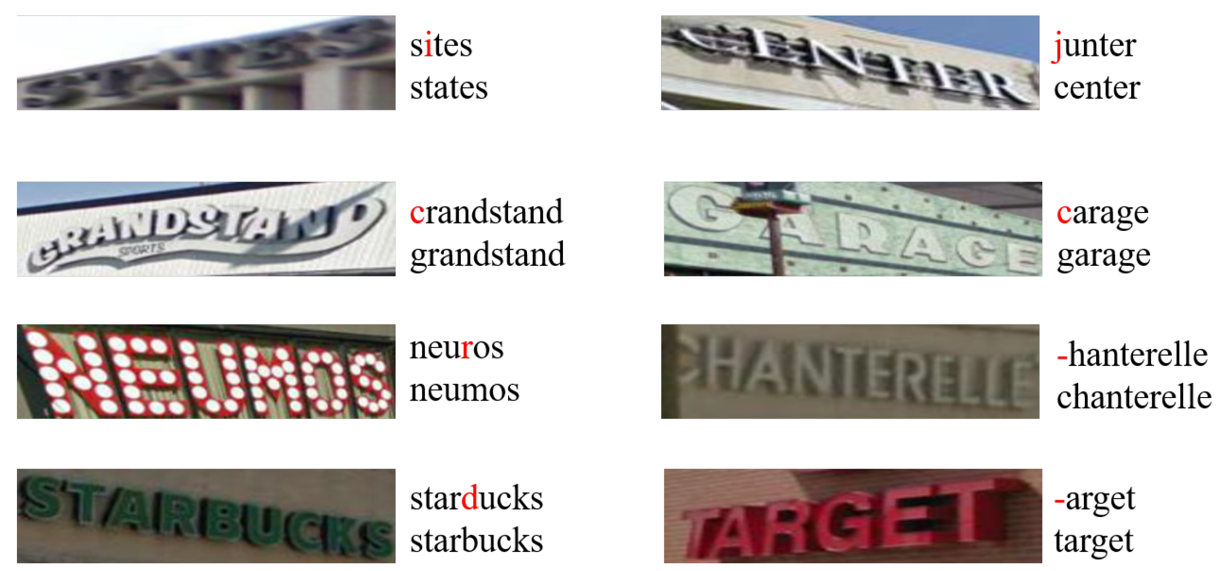
4.4.6. Discussion on Attention Visualization

Figure 7 shows the attention map from each embedding to the input images. We used Attention Rollout [53] following ViT. We averaged the attention weights of TRIG across all heads and recursively compute the attention matrix. At last, we can get pixel attribution for embeddings in (b). The first row shows what part of the rectified picture is responsible for the initial embedding. Furthermore, the rest of the rows represent the attention map of feature embeddings $[f_1,f_2,\dots ,f_N]$. The initial embedding is mainly relevant to the first character. For each feature embedding, some of the features come from adjacent embeddings and others come from distant embeddings. According to Figure 7, we can roughly learn how the transformer feature extractor extract features and model long-range dependencies.

4.4.7. Discussion on Efficiency

To verify the efficiency of our model, we compare the MACs, parameters, GPU memory, and inference speed of our model using 1-D split (square patch with the size of 4 × 4) and 2-D split (rectangle patch with the size of 32 × 4) and ASTER. The result is shown in

Table 4. Efficiency comparison between ASTER and TRIG. MACS, model parameters, gpu memory cost, and speed are compared.

Method	MACs G	#Param. M	GPU Memory (Train) m	GPU Memory (Inference) m	Inference Time ms/Image
ASTER	1.6	21.0	1509	3593	19.5
TRIG	2.6	68.1	2579	1855	16.2
2-D split	18.2	68.0	8717	1929	37.6

. The MACs of TRIG with 1-D split and training GPU memory cost (the batch size is 32) are 7 times and 3.4 times of the method with 2-D split. Furthermore, the speed of TRIG is faster than ASTER. The speed performance is tested on GeForce GTX 1080 Ti GPU.

4.5. Ablation Study

In this section, we perform a series of experiments to evaluate the impact of blocks, heads, embedding dimension, initial embedding guide, and skip attention on recognition performance. All models are trained from scratch on two synthetic datasets. The results are reported on seven standard benchmarks and shown in Tabel

Table 5. Performance comparison with different settings. ’Initial guidance’ indicates the initial embedding guidance. ’Skip attention’ denotes the skip attention in the TFE. ’Average’ means the average accuracy of seven standard benchmarks. * denotes the setting of TRIG shown in Table 1.

Blocks	Heads	Embedding Dimension	Initial Guidance	Skip Attention	Average
6	16	512	×	×	89.2
6	16	512	×	✓	89.8 (+0.6)
12	16	256	×	×	89.4 (+0.2)
12	8	256	×	✓	90.1 (+0.9)
12	16	256	×	✓	90.4 (+1.2)
12	16	512	×	×	89.5 (+0.3)
12	16	512	✓	×	89.6 (+0.4)
12	16	512	×	✓	90.6 (+1.4)
12	16	512	✓	✓	90.8 (+1.6) *
24	16	512	✓	✓	90.6 (+1.4)

. We can make the following observations: (1) The TRIG with 12 blocks is better than the model of six blocks. The performance can be improved by stacking more transformer encoder blocks. However, when transformer encoder goes deeper, the stacking blocks cannot increase the performance (the average accuracy of 24 blocks decreases by 0.2 pp). The accuracy may reach the bottleneck. It is expected that stacking blocks lead to more challenging training procedures. (2) Initial embedding can bring gains to the model on average accuracy no matter skip attention is applied or not. This shows the effectiveness of initial embedding guidance. (3) Skip attention is important to accuracy. Regardless of the depth of the feature extractor, the addition of skip attention brings gains to the performance. (4) When other conditions are guaranteed to be the same, the average accuracy of 16 heads is better than the condition of 8 heads. Besides, the average accuracy of 512 dimensions is better than 256 dimensions.

5. Conclusions

In this work, we propose a three-stage transformer-based text recognizer with initial embedding guidance named TRIG. In contrast to the existing STR network, this method only uses transformer feature extractor to extract robust features and does not need a context modeling module. A 1-D split is designed to divide text images. Besides, we propose a learnable initial embedding learned from transformer encoder to guide the attention decoder. Extensive experiments demonstrate that our method sets the new state of the art on several benchmarks.

We also demonstrate that the longer training epochs and long-range dependencies are essential to TRIG.

We consider three promising directions for future work. First, a better transformer architecture that is more suitable for Scene text recognition can be designed to extract more robust features. For example, a transformer can be designed as a pyramid structure such as CNN or some other structure. Second, we see potential in using a transformer in an end-to-end text spotting system. Third, TRIG can be improved to solve the problem about other languages [54] and hand-written (cursive) text recognition [55,56].

References

1. Long, S.; He, X.; Yao, C. Scene Text Detection and Recognition: The Deep Learning Era. Int. J. Comput. Vis. 2021, 129, 161–184. [Google Scholar] [CrossRef]
2. Zhu, Y.; Yao, C.; Bai, X. Scene text detection and recognition: Recent advances and future trends. Front. Comput. Sci. 2016, 10, 19–36. [Google Scholar] [CrossRef]
3. Shi, B.; Yang, M.; Wang, X.; Lyu, P.; Yao, C.; Bai, X. ASTER: An Attentional Scene Text Recognizer with Flexible Rectification. IEEE Trans. Pattern Anal. Mach. Intell. 2019, 41, 2035–2048. [Google Scholar] [CrossRef] [PubMed]
4. He, K.; Zhang, X.; Ren, S.; Sun, J. Deep Residual Learning for Image Recognition. In Proceedings of the 2016 IEEE Conference on Computer Vision and Pattern Recognition, Las Vegas, NV, USA, 27–30 June 2016; pp. 770–778. [Google Scholar] [CrossRef] [Green Version]
5. Yu, D.; Li, X.; Zhang, C.; Liu, T.; Han, J.; Liu, J.; Ding, E. Towards Accurate Scene Text Recognition With Semantic Reasoning Networks. In Proceedings of the 2020 IEEE/CVF Conference on Computer Vision and Pattern Recognition, Seattle, WA, USA, 13–19 June 2020; pp. 12110–12119. [Google Scholar] [CrossRef]
6. Lin, T.; Dollár, P.; Girshick, R.B.; He, K.; Hariharan, B.; Belongie, S.J. Feature Pyramid Networks for Object Detection. In Proceedings of the 2017 IEEE Conference on Computer Vision and Pattern Recognition, CVPR 2017, Honolulu, HI, USA, 21–26 July 2017; pp. 936–944. [Google Scholar] [CrossRef] [Green Version]
7. Hochreiter, S.; Schmidhuber, J. Long Short-Term Memory. Neural Comput. 1997, 9, 1735–1780. [Google Scholar] [CrossRef] [PubMed]
8. Vaswani, A.; Shazeer, N.; Parmar, N.; Uszkoreit, J.; Jones, L.; Gomez, A.N.; Kaiser, L.; Polosukhin, I. Attention is All you Need. In Proceedings of the Advances in Neural Information Processing Systems 30: Annual Conference on Neural Information Processing Systems 2017, Long Beach, CA, USA, 4–9 December 2017; Neural Information Processing Systems: San Diego, CA, USA, 2017; pp. 5998–6008. [Google Scholar]
9. Dosovitskiy, A.; Beyer, L.; Kolesnikov, A.; Weissenborn, D.; Zhai, X.; Unterthiner, T.; Dehghani, M.; Minderer, M.; Heigold, G.; Gelly, S.; et al. An Image is Worth 16x16 Words: Transformers for Image Recognition at Scale. In Proceedings of the 9th International Conference on Learning Representations, ICLR 2021, Virtual Event. Vienna, Austria, 3–7 May 2021. [Google Scholar]
10. Baek, J.; Kim, G.; Lee, J.; Park, S.; Han, D.; Yun, S.; Oh, S.J.; Lee, H. What Is Wrong with Scene Text Recognition Model Comparisons? Dataset and Model Analysis. In Proceedings of the 2019 IEEE/CVF International Conference on Computer Vision, ICCV 2019, Seoul, Korea, 27 October–2 November 2019; pp. 4714–4722. [Google Scholar] [CrossRef] [Green Version]
11. Touvron, H.; Cord, M.; Douze, M.; Massa, F.; Sablayrolles, A.; Jégou, H. Training data-efficient image transformers & distillation through attention. In Proceedings of the 38th International Conference on Machine Learning, ICML 2021; Virtual Event; Austria, 18–24 July 2021, International Conference on Machine Learning: San Diego, CA, USA, 2021; Volume 139, pp. 10347–10357. [Google Scholar]
12. Beal, J.; Kim, E.; Tzeng, E.; Park, D.H.; Zhai, A.; Kislyuk, D. Toward Transformer-Based Object Detection. arXiv 2020, arXiv:2012.09958. [Google Scholar]
13. Zhao, H.; Jiang, L.; Jia, J.; Torr, P.H.S.; Koltun, V. Point Transformer. arXiv 2020, arXiv:2012.09164. [Google Scholar]
14. Valanarasu, J.M.J.; Oza, P.; Hacihaliloglu, I.; Patel, V.M. Medical Transformer: Gated Axial-Attention for Medical Image Segmentation. In Lecture Notes in Computer Science, Proceedings of the Medical Image Computing and Computer Assisted Intervention—MICCAI 2021-24th International Conference, Strasbourg, France, 27 September–1 October 2021; de Bruijne, M., Cattin, P.C., Cotin, S., Padoy, N., Speidel, S., Zheng, Y., Essert, C., Eds.; Part I; Springer: Berlin/Heidelberg, Germany, 2021; Volume 12901, pp. 36–46. [Google Scholar] [CrossRef]
15. Li, H.; Wang, P.; Shen, C.; Zhang, G. Show, Attend and Read: A Simple and Strong Baseline for Irregular Text Recognition. In Proceedings of the Thirty-Third AAAI Conference on Artificial Intelligence, AAAI 2019, Honolulu, HI, USA, 27 January–1 February 2019; AAAI Press: Palo Alto, CA, USA, 2019; pp. 8610–8617. [Google Scholar] [CrossRef] [Green Version]
16. Lu, N.; Yu, W.; Qi, X.; Chen, Y.; Gong, P.; Xiao, R.; Bai, X. MASTER: Multi-aspect non-local network for scene text recognition. Pattern Recognit. 2021, 117, 107980. [Google Scholar] [CrossRef]
17. Coates, A.; Carpenter, B.; Case, C.; Satheesh, S.; Suresh, B.; Wang, T.; Wu, D.J.; Ng, A.Y. Text Detection and Character Recognition in Scene Images with Unsupervised Feature Learning. In Proceedings of the 2011 International Conference on Document Analysis and Recognition, Beijing, China, 18–21 September 2011; pp. 440–445. [Google Scholar] [CrossRef] [Green Version]
18. Wang, K.; Belongie, S.J. Word Spotting in the Wild. In Lecture Notes in Computer Science, Proceedings of the Computer Vision-ECCV 2010, 11th European Conference on Computer Vision, Heraklion, Crete, Greece, 5–11 September 2010; Daniilidis, K., Maragos, P., Paragios, N., Eds.; Part I; Springer: Berlin/Heidelberg, Germany, 2010; Volume 6311, pp. 591–604. [Google Scholar] [CrossRef]
19. Lee, C.; Bhardwaj, A.; Di, W.; Jagadeesh, V.; Piramuthu, R. Region-Based Discriminative Feature Pooling for Scene Text Recognition. In Proceedings of the 2014 IEEE Conference on Computer Vision and Pattern Recognition, CVPR 2014, Columbus, OH, USA, 23–28 June 2014; IEEE Computer Society: Washington, DC, USA, 2014; pp. 4050–4057. [Google Scholar] [CrossRef]
20. Mishra, A.; Alahari, K.; Jawahar, C.V. Top-down and bottom-up cues for scene text recognition. In Proceedings of the 2012 IEEE Conference on Computer Vision and Pattern Recognition, Providence, RI, USA, 16–21 June 2012; IEEE Computer Society: Washington, DC, USA, 2012; pp. 2687–2694. [Google Scholar] [CrossRef] [Green Version]
21. Phan, T.Q.; Shivakumara, P.; Tian, S.; Tan, C.L. Recognizing Text with Perspective Distortion in Natural Scenes. In Proceedings of the IEEE International Conference on Computer Vision, ICCV 2013, Sydney, Australia, 1–8 December 2013; IEEE Computer Society: Washington, DC, USA, 2013; pp. 569–576. [Google Scholar] [CrossRef]
22. Shi, B.; Bai, X.; Yao, C. An End-to-End Trainable Neural Network for Image-Based Sequence Recognition and Its Application to Scene Text Recognition. IEEE Trans. Pattern Anal. Mach. Intell. 2017, 39, 2298–2304. [Google Scholar] [CrossRef] [PubMed] [Green Version]
23. Graves, A.; Fernández, S.; Gomez, F.J.; Schmidhuber, J. Connectionist temporal classification: Labelling unsegmented sequence data with recurrent neural networks. In Proceedings of the Twenty-Third International Conference (ICML 2006), Pittsburgh, PA, USA, 25–29 June 2006; Cohen, W.W., Moore, A.W., Eds.; ACM: New York, NY, USA, 2006; Volume 148, pp. 369–376. [Google Scholar] [CrossRef]
24. Jaderberg, M.; Simonyan, K.; Zisserman, A.; Kavukcuoglu, K. Spatial Transformer Networks. In Proceedings of the Advances in Neural Information Processing Systems 28: Annual Conference on Neural Information Processing Systems 2015, Montreal, QC, Canada, 7–12 December 2015; Cortes, C., Lawrence, N.D., Lee, D.D., Sugiyama, M., Garnett, R., Eds.; Neural Information Processing Systems: San Diego, CA, USA, 2015; pp. 2017–2025. [Google Scholar]
25. Wan, Z.; Xie, F.; Liu, Y.; Bai, X.; Yao, C. 2D-CTC for Scene Text Recognition. arXiv 2019, arXiv:1907.09705. [Google Scholar]
26. Liao, M.; Lyu, P.; He, M.; Yao, C.; Wu, W.; Bai, X. Mask TextSpotter: An End-to-End Trainable Neural Network for Spotting Text with Arbitrary Shapes. IEEE Trans. Pattern Anal. Mach. Intell. 2021, 43, 532–548. [Google Scholar] [CrossRef] [PubMed] [Green Version]
27. Qiao, Z.; Zhou, Y.; Yang, D.; Zhou, Y.; Wang, W. SEED: Semantics Enhanced Encoder-Decoder Framework for Scene Text Recognition. In Proceedings of the 2020 IEEE/CVF Conference on Computer Vision and Pattern Recognition, Seattle, WA, USA, 13–19 June 2020; pp. 13525–13534. [Google Scholar] [CrossRef]
28. Carion, N.; Massa, F.; Synnaeve, G.; Usunier, N.; Kirillov, A.; Zagoruyko, S. End-to-End Object Detection with Transformers. In Lecture Notes in Computer Science, Proceedings of the Computer Vision-ECCV 2020-16th European Conference, Glasgow, UK, 23–28 August 2020; Vedaldi, A., Bischof, H., Brox, T., Frahm, J., Eds.; Part I; Springer: Cham, Switzerland, 2020; Volume 12346, pp. 213–229. [Google Scholar] [CrossRef]
29. Ren, S.; He, K.; Girshick, R.B.; Sun, J. Faster R-CNN: Towards Real-Time Object Detection with Region Proposal Networks. IEEE Trans. Pattern Anal. Mach. Intell. 2017, 39, 1137–1149. [Google Scholar] [CrossRef] [PubMed] [Green Version]
30. Lee, J.; Park, S.; Baek, J.; Oh, S.J.; Kim, S.; Lee, H. On Recognizing Texts of Arbitrary Shapes with 2D Self-Attention. In Proceedings of the 2020 IEEE/CVF Conference on Computer Vision and Pattern Recognition, CVPR Workshops 2020, Seattle, WA, USA, 14–19 June 2020; pp. 2326–2335. [Google Scholar] [CrossRef]
31. Sheng, F.; Chen, Z.; Xu, B. NRTR: A No-Recurrence Sequence-to-Sequence Model for Scene Text Recognition. In Proceedings of the 2019 International Conference on Document Analysis and Recognition, ICDAR 2019, Sydney, Australia, 20–25 September 2019; pp. 781–786. [Google Scholar] [CrossRef] [Green Version]
32. Bookstein, F.L. Principal Warps: Thin-Plate Splines and the Decomposition of Deformations. IEEE Trans. Pattern Anal. Mach. Intell. 1989, 11, 567–585. [Google Scholar] [CrossRef] [Green Version]
33. He, R.; Ravula, A.; Kanagal, B.; Ainslie, J. RealFormer: Transformer Likes Residual Attention. In Proceedings of the Findings of the Association for Computational Linguistics: ACL/IJCNLP 2021, Online Event. 1–6 August 2021; Zong, C., Xia, F., Li, W., Navigli, R., Eds.; Association for Computational Linguistics: Stroudsburg, PA, USA, 2021; pp. 929–943. [Google Scholar] [CrossRef]
34. Cho, K.; van Merrienboer, B.; Gülçehre, Ç.; Bahdanau, D.; Bougares, F.; Schwenk, H.; Bengio, Y. Learning Phrase Representations using RNN Encoder-Decoder for Statistical Machine Translation. In Proceedings of the 2014 Conference on Empirical Methods in Natural Language Processing, EMNLP 2014, Doha, Qatar, 25–29 October 2014; Moschitti, A., Pang, B., Daelemans, W., Eds.; A Meeting of SIGDAT, a Special Interest Group of the ACL. ACL: Stroudsburg, PA, USA, 2014; pp. 1724–1734. [Google Scholar] [CrossRef]
35. Jaderberg, M.; Simonyan, K.; Vedaldi, A.; Zisserman, A. Synthetic Data and Artificial Neural Networks for Natural Scene Text Recognition. arXiv 2014, arXiv:1406.2227. [Google Scholar]
36. Gupta, A.; Vedaldi, A.; Zisserman, A. Synthetic Data for Text Localisation in Natural Images. In Proceedings of the 2016 IEEE Conference on Computer Vision and Pattern Recognition, CVPR 2016, Las Vegas, NV, USA, 27–30 June 2016; IEEE Computer Society: Washington, DC, USA, 2016; pp. 2315–2324. [Google Scholar] [CrossRef] [Green Version]
37. Mishra, A.; Alahari, K.; Jawahar, C.V. Scene Text Recognition using Higher Order Language Priors. In Proceedings of the British Machine Vision Conference, BMVC 2012, Surrey, UK, 3–7 September 2012; Bowden, R., Collomosse, J.P., Mikolajczyk, K., Eds.; BMVA Press: Durham, UK, 2012; pp. 1–11. [Google Scholar] [CrossRef] [Green Version]
38. Wang, K.; Babenko, B.; Belongie, S.J. End-to-end scene text recognition. In Proceedings of the IEEE International Conference on Computer Vision, ICCV 2011, Barcelona, Spain, 6–13 November 2011; Metaxas, D.N., Quan, L., Sanfeliu, A., Gool, L.V., Eds.; IEEE Computer Society: Washington, DC, USA, 2011; pp. 1457–1464. [Google Scholar] [CrossRef]
39. Lucas, S.M.; Panaretos, A.; Sosa, L.; Tang, A.; Wong, S.; Young, R.; Ashida, K.; Nagai, H.; Okamoto, M.; Yamamoto, H.; et al. ICDAR 2003 robust reading competitions: Entries, results, and future directions. Int. J. Doc. Anal. Recognit. 2005, 7, 105–122. [Google Scholar] [CrossRef]
40. Karatzas, D.; Shafait, F.; Uchida, S.; Iwamura, M.; Bigorda, L.G.; Mestre, S.R.; Mas, J.; Mota, D.F.; Almazán, J.; de las Heras, L. ICDAR 2013 Robust Reading Competition. In Proceedings of the 12th International Conference on Document Analysis and Recognition, ICDAR 2013, Washington, DC, USA, 25–28 August 2013; IEEE Computer Society: Washington, DC, USA, 2013; pp. 1484–1493. [Google Scholar] [CrossRef] [Green Version]
41. Karatzas, D.; Gomez-Bigorda, L.; Nicolaou, A.; Ghosh, S.K.; Bagdanov, A.D.; Iwamura, M.; Matas, J.; Neumann, L.; Chandrasekhar, V.R.; Lu, S.; et al. ICDAR 2015 competition on Robust Reading. In Proceedings of the 13th International Conference on Document Analysis and Recognition, ICDAR 2015, Nancy, France, 23–26 August 2015; IEEE Computer Society: Washington, DC, USA, 2015; pp. 1156–1160. [Google Scholar] [CrossRef]
42. Risnumawan, A.; Shivakumara, P.; Chan, C.S.; Tan, C.L. A robust arbitrary text detection system for natural scene images. Expert Syst. Appl. 2014, 41, 8027–8048. [Google Scholar] [CrossRef]
43. Cheng, Z.; Bai, F.; Xu, Y.; Zheng, G.; Pu, S.; Zhou, S. Focusing Attention: Towards Accurate Text Recognition in Natural Images. In Proceedings of the IEEE International Conference on Computer Vision, ICCV 2017, Venice, Italy, 22–29 October 2017; IEEE Computer Society: Washington, DC, USA, 2017; pp. 5086–5094. [Google Scholar] [CrossRef] [Green Version]
44. Zhan, F.; Lu, S. ESIR: End-To-End Scene Text Recognition via Iterative Image Rectification. In Proceedings of the IEEE Conference on Computer Vision and Pattern Recognition, CVPR 2019, Long Beach, CA, USA, 16–20 June 2019; pp. 2059–2068. [Google Scholar] [CrossRef] [Green Version]
45. Luo, C.; Jin, L.; Sun, Z. MORAN: A Multi-Object Rectified Attention Network for scene text recognition. Pattern Recognit. 2019, 90, 109–118. [Google Scholar] [CrossRef]
46. Wang, T.; Zhu, Y.; Jin, L.; Luo, C.; Chen, X.; Wu, Y.; Wang, Q.; Cai, M. Decoupled Attention Network for Text Recognition. In Proceedings of the Thirty-Fourth AAAI Conference on Artificial Intelligence, AAAI 2020, New York, NY, USA, 7–12 February 2020; AAAI Press: Palo Alto, CA, USA, 2020; pp. 12216–12224. [Google Scholar]
47. Yue, X.; Kuang, Z.; Lin, C.; Sun, H.; Zhang, W. RobustScanner: Dynamically Enhancing Positional Clues for Robust Text Recognition. In Lecture Notes in Computer Science, Proceedings of the Computer Vision-ECCV 2020-16th European Conference, Glasgow, UK, 23–28 August 2020; Vedaldi, A., Bischof, H., Brox, T., Frahm, J., Eds.; Part XIX; Springer: Cham, Switzerland, 2020; Volume 12364, pp. 135–151. [Google Scholar] [CrossRef]
48. Mou, Y.; Tan, L.; Yang, H.; Chen, J.; Liu, L.; Yan, R.; Huang, Y. PlugNet: Degradation Aware Scene Text Recognition Supervised by a Pluggable Super-Resolution Unit. In Lecture Notes in Computer Science, Proceedings of the Computer Vision-ECCV 2020-16th European Conference, Glasgow, UK, 23–28 August 2020; Vedaldi, A., Bischof, H., Brox, T., Frahm, J., Eds.; Part XV; Springer: Cham, Switzerland, 2020; Volume 12360, pp. 158–174. [Google Scholar] [CrossRef]
49. Zhang, H.; Yao, Q.; Yang, M.; Xu, Y.; Bai, X. AutoSTR: Efficient Backbone Search for Scene Text Recognition. In Lecture Notes in Computer Science, Proceedings of the Computer Vision-ECCV 2020-16th European Conference, Glasgow, UK, 23–28 August 2020; Vedaldi, A., Bischof, H., Brox, T., Frahm, J., Eds.; Part XXIV; Springer: Cham, Switzerland, 2020; Volume 12369, pp. 751–767. [Google Scholar] [CrossRef]
50. Zhang, C.; Xu, Y.; Cheng, Z.; Pu, S.; Niu, Y.; Wu, F.; Zou, F. SPIN: Structure-Preserving Inner Offset Network for Scene Text Recognition. In Proceedings of the Thirty-Fifth AAAI Conference on Artificial Intelligence, AAAI 2021, Virtual Event. Vienna, Austria, 2–9 February 2021; AAAI Press: Palo Alto, CA, USA, 2021; pp. 3305–3314. [Google Scholar]
51. Hu, W.; Cai, X.; Hou, J.; Yi, S.; Lin, Z. GTC: Guided Training of CTC towards Efficient and Accurate Scene Text Recognition. In Proceedings of the Thirty-Fourth AAAI Conference on Artificial Intelligence, AAAI 2020, The Thirty-Second Innovative Applications of Artificial Intelligence Conference, IAAI 2020, The Tenth AAAI Symposium on Educational Advances in Artificial Intelligence, EAAI 2020, New York, NY, USA, 7–12 February 2020; AAAI Press: Palo Alto, CA, USA, 2020; pp. 11005–11012. [Google Scholar]
52. Litman, R.; Anschel, O.; Tsiper, S.; Litman, R.; Mazor, S.; Manmatha, R. SCATTER: Selective Context Attentional Scene Text Recognizer. In Proceedings of the 2020 IEEE/CVF Conference on Computer Vision and Pattern Recognition, CVPR 2020, Seattle, WA, USA, 13–19 June 2020; pp. 11959–11969. [Google Scholar] [CrossRef]
53. Abnar, S.; Zuidema, W.H. Quantifying Attention Flow in Transformers. In Proceedings of the 58th Annual Meeting of the Association for Computational Linguistics, ACL 2020, Online. 5–10 July 2020; Jurafsky, D., Chai, J., Schluter, N., Tetreault, J.R., Eds.; Association for Computational Linguistics: Stroudsburg, PA, USA, 2020; pp. 4190–4197. [Google Scholar] [CrossRef]
54. Sun, Y.; Liu, J.; Liu, W.; Han, J.; Ding, E.; Liu, J. Chinese Street View Text: Large-Scale Chinese Text Reading With Partially Supervised Learning. In Proceedings of the 2019 IEEE/CVF International Conference on Computer Vision, ICCV 2019, Seoul, Korea, 27 October–2 November 2019; pp. 9085–9094. [Google Scholar] [CrossRef] [Green Version]
55. Huang, J.; Haq, I.U.; Dai, C.; Khan, S.; Nazir, S.; Imtiaz, M. Isolated Handwritten Pashto Character Recognition Using a K-NN Classification Tool based on Zoning and HOG Feature Extraction Techniques. Complexity 2021, 2021, 5558373. [Google Scholar] [CrossRef]
56. Khan, S.; Hafeez, A.; Ali, H.; Nazir, S.; Hussain, A. Pioneer dataset and recognition of Handwritten Pashto characters using Convolution Neural Networks. Meas. Control 2020, 53, 2041–2054. [Google Scholar] [CrossRef]
Figure 1. Difference between 1 and D split and 2-D split. (a) A rectified text image. (b) 2-D split: The text image is split into square patches proposed in the ViT-like backbone. (c) 1-D split: The text image is split into rectangle patches whose height is the same as the height of the rectified image. Using the same patch dimension, the 1-D split is more efficient than the 2-D split.
Electronics 10 02780 g001
Figure 2. The overview of three-stage text recognizer, TRIG. The first stage is transformation (TRA), which is used to rectify text images. The second stage is a Transformer Feature Extractor (TFE), aiming to extract effective and robust features and implicitly model context. The third stage is an attention decoder (AD), which is used to decode the sequence of features into characters. Text can be predicted from the image by TRIG.
Electronics 10 02780 g002
Figure 3. The detailed architectures of the TFE and AD module. TFE consists of Patch Embedding, Position Embedding, Transformer Encoder Blocks, and Residual add module. The skip edge in the Residual add module connects Multi-Head Self-Attention modules in adjacent Transformer Encoder Blocks. Here, ⊗ denotes matrix multiplication, ⊕ denotes broadcast element-wise addition.
Electronics 10 02780 g003
Figure 4. The accuracy on IIIT between TRIG (Ours) and ASTER during the training process.
Electronics 10 02780 g004
Figure 5. The detail of the mask used in the transformer encoder. The gray square denotes the mask. The first row means initial embedding which can see all embeddings. The remaining features can only see other features of the window size.
Electronics 10 02780 g005
Figure 6. Right cases of TRIG with/without initial embedding guided. The predictions are placed along the right side of the images. The top string is the prediction of TRIG without the initial embedding guidance. The bottom string is the prediction of TRIG.
Electronics 10 02780 g006
Figure 7. The attention visualization of TFE. (a) Examples of rectified images. (b) The attention map of initial embedding and each embedding in feature map extracted with the transformer encoder.
Electronics 10 02780 g007