Iterative Learning Sliding Mode Control for UAV Trajectory Tracking

Abstract

This paper presents a novel iterative learning sliding mode controller (ILSMC) that can be applied to the trajectory tracking of quadrotor unmanned aerial vehicles (UAVs) subject to model uncertainties and external disturbances. Here, the proposed ILSMC is integrated in the outer loop of a controlled system. The control development, conducted in the discrete-time domain, does not require a priori information of the disturbance bound as with conventional SMC techniques. It only involves an equivalent control term for the desired dynamics in the closed loop and an iterative learning term to drive the system state toward the sliding surface to maintain robust performance. By learning from previous iterations, the ILSMC can yield very accurate tracking performance when a sliding mode is induced without control chattering. The design is then applied to the attitude control of a 3DR Solo UAV with a built-in PID controller. The simulation results and experimental validation with real-time data demonstrate the advantages of the proposed control scheme over existing techniques.

1. Introduction

In recent years, the interest in developing and utilizing unmanned aerial vehicles (UAVs) has been growing, with numerous applications in practice, such as mapping [1,2], inspection, search and rescue [3,4], construction automation [5], and agricultural surveillance [6]. When a quadrotor drone performs a desired trajectory, accurate tracking is highly necessary. In trajectory tracking control, feedback linearization (FL) has been widely used [7,8]. This control method works well under the assumption of known system dynamics. When faced with large uncertainties and disturbances, FL-based approaches may lead to poor tracking performance, and other advanced control laws are required. An adaptive feedback linearization controller was applied in [9], allowing for adjustments of the control parameters to enhance control performance. Robust control methods were also developed to improve control performance [10]. A backstepping controller was introduced in [11] to improve the tracking accuracy and robustness of UAVs’ attitude control, wherein the external disturbances are estimated using a nonlinear disturbance observer.

Sliding mode control (SMC), a well-known control method for improving system robustness, has been successfully applied to various control systems [12,13] in general and particularly to UAVs [14,15]. However, information on disturbance bounds is required in these techniques. Adaptive SMC was developed to overcome this requirement [16]. This approach still reveals the main disadvantage of SMC, i.e., control signals usually present a chattering behavior, especially when dealing with large uncertainties and disturbances, which often require excessively high control gains. Various techniques have been suggested as a remedy, mostly using an approximation of the sign function to avoid or reduce chattering with some trade-offs with system robustness for control signal smoothing. Deep-learning-based techniques with convolutional neural networks have recently shown promise in learning systems that are subject to highly complex and time-varying uncertainties, for example, in vision-based applications such as in robust face tracking [17]. For control in robotic manipulators, a deep convolutional neural network was developed to integrate learning schemes into a fractional-order terminal sliding-mode controller for enhancing tracking accuracy [18]. Although the deep learning methods can achieve high-quality performance with continuous control signals, a major disadvantage is the high computational cost incurred for implementing a deep neural network.

Iterative learning control (ILC) is an effective technique for dealing with repetitive tasks. It allows for learning from system data to update the control input repeatedly to improve system performance [19]. Through trial-based learning, ILC is able to achieve highly accurate tracking performance even with large model uncertainties and disturbances. Unlike nonlearning control techniques, the system in ILC is reset to zero after the system reaches the final time, and then repeatedly follows the same reference again. Thereby, the control input can be adjusted through the repetitions to result in perfect tracking. Since ILC can learn from the system response to provide feedforward control in the iteration domain, it is more robust and can effectively compensate for model uncertainties and unknown disturbances, particularly iteration-invariant disturbances [20].

The application of iterative cybernetics, first proposed in [21], has emerged for iterative learning control in robotic systems [22], later developed for industrial control [23]. In the past decades, ILC has become an effective tool in various control systems, such as robot arm manipulators [24], chemical batch processes [25], wafer scanner systems [26], and video-rate atomic force microscopy [27]. Unlike other learning techniques such as artificial neural networks, which obtain the inverse dynamics from a training set [28] or adaptive controller, which tunes the control parameters [29,30], requiring a time-consuming process, ILC updates the control input from the information from previous executions and can hence converge quickly after a limited number of repetitions [19]. Moreover, as ILC does not require a system model, it is quite beneficial in practical applications that deal with unknown characteristics.

In this paper, integrating the learning capacity of ILC with the strong robustness of SMC, we propose a novel iterative learning sliding mode controller (ILSMC) to achieve high-accuracy trajectory tracking for UAVs while retaining strong robustness as well as alleviating control chattering. In terms of iterative control, several existing techniques have been introduced for UAVs. In [31], a plug-in controller was designed and implemented in aerial robots. Although the average tracking error is reduced for periodic reference trajectories, the technique does not concern the effect of disturbances. In [32], fuzzy PID-typed ILC was introduced; where fuzzy logic is used to tune the control parameters, high-accuracy tracking performance is hard to attain in comparison to other rigorous control strategies. In [33], optimization-based ILC was developed to improve the UAV trajectory tracking performance. In this approach, learning and filtering schemes are formulated into convex optimal problems. Although the two-step convex optimization problem can be solved using software, it involves high computational complexity.

The proposed ILSMC offers a simpler design, and thus is more robust and effective. The main contributions of this work include (i) the comprehensive development of an iterative learning term with fast convergence after several iterations to compensate for system uncertainties and unknown disturbances, and (ii) the integration of ILC and SMC schemes to a built-in PID controller in cascade to yield high performance for quadcopter trajectory tracking.

This paper is structured as follows: The control development of ILSMC is presented in Section 2. The convergence and stability analysis of the proposed learning algorithm is also provided in this section. Next, Section 3 presents system modeling, including kinematic and quadcopter dynamics. Then, the integration of ILSMC with PID control for the UAV is described in Section 4. Section 5 provides numerical simulation results, and Section 6 presents experimental validation with real-time data. Finally, a conclusion is drawn in Section 7.

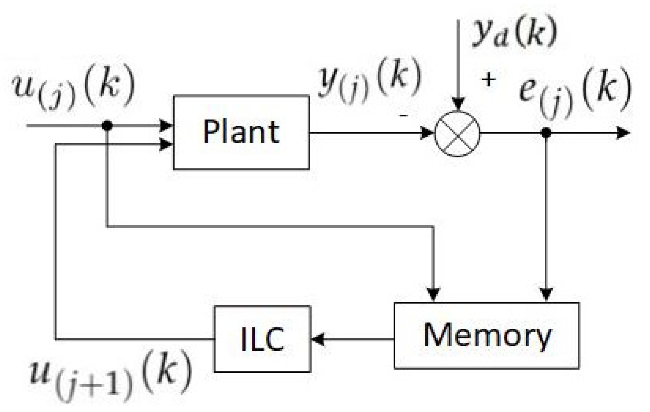
2. Iterative Learning Sliding Mode Control

Iterative learning control (ILC) is a tracking control strategy for systems performing repetitive tasks, which are commonly required in industry. This technique aims to generate a feedforward control signal so that the system can learn from the previous responses to improve tracking performance and repeatedly eliminate disturbance after each iteration. The basic structure of an ILC is depicted in Figure 1 for an iteration number j. At this iteration, the input $u_{\left(j\right)}\left(k\right)$ and the deviation $e_{\left(j\right)}\left(k\right)$ between the reference $y_d\left(k\right)$ and the output $y_{\left(j\right)}\left(k\right)$ are stored to compute the control signal for the next iteration, with k starting from an initial time instant ($k=0$). In this section, an iterative learning sliding mode control scheme is designed to deal with large uncertainties and disturbances.

2.1. ILSMC Design

Consider the following general discrete-time control system:

$$\left\{\begin{array}{c}{x}_{1_{\left(j\right)}}(k+1)=x_{1_{\left(j\right)}}\left(k\right)+{\mathsf{\Delta }}_t{x}_{2_{\left(j\right)}}\left(k\right),\hfill \\ x_{2_{\left(j\right)}}(k+1)=f\left(x_{\left(j\right)}\left(k\right)\right)+{\mathsf{\Delta }}_{t}B\left[u_{\left(j\right)}\left(k\right)+d_{\left(j\right)}\left(k\right)\right],\hfill \end{array}\right.$$

(1)

where k is the time instant and ${\mathsf{\Delta }}_t$ is the sampling period. The subscript j denotes the iteration index, also called trial, run, cycle, or repetition in the ILC literature. The system state vector is $x_{\left(j\right)}\left(k\right)={\left[\begin{array}{cc}{x}_{1_{\left(j\right)}}\left(k\right)& x_{2_{\left(j\right)}}\left(k\right)\end{array}\right]}^T\in {\mathbb{R}}^{2m}$, where m is the dimension of state $x_{1_{\left(j\right)}}\left(k\right)$, $x_{2_{\left(j\right)}}\left(k\right)$ is its derivative, $u_{\left(j\right)}\left(k\right)\in {\mathbb{R}}^m$ is the control signal, $B\in {\mathbb{R}}^{m\times m}$ is a positive definite matrix, and $f(.)$ is a vector function. The influence of parameter variations and loading conditions, model uncertainties and external disturbances can be lumped into a vector $d_{\left(j\right)}\left(k\right)$. In each iteration, the input and state variables comprise an N-sample sequence each, where N is a finite number of samples.

Definition 1.

At iteration j, an exogenous input ${\delta }_{\left(j\right)}\left(k\right)$ is called iteration-invariant if it occurs repeatedly over iterations, or persistent within the iteration domain, that is, ${\delta }_{\left(1\right)}\left(k\right)={\delta }_{\left(2\right)}\left(k\right)=\dots ={\delta }_{\left(j\right)}\left(k\right)$ for all $k=\{0,1,...,N-1\}$.

To proceed with the ILC methodology, the following assumption [20,27,34] is made:

Assumption 1.

In this paper, the lumped disturbance $d_{\left(j\right)}\left(k\right)$ is assumed to be iteration-invariant.

In this paper, an ILSMC law is developed aiming to drive the tracking error asymptotically to zero from any initial condition and under external disturbances $d_{\left(j\right)}\left(k\right)$. The control algorithm consists of two steps. The first step is to induce a desired sliding surface to drive a learning sliding function to zero after some iterations regardless of external disturbance and system uncertainties. In the second step, the tracking error of the system is driven to zero in the sliding mode associated with the control sliding function. Instead of using a discontinuous gain as in the conventional SMC methodology, here, an iteration learning process is involved; hence, a priori information of the disturbance bound is not required, and chattering is fully alleviated.

The control design is initiated by considering the tracking error in an iteration as

$$e_{\left(j\right)}\left(k\right)={\left[\begin{array}{cc}{e}_{1\left(j\right)}\left(k\right)& e_{2\left(j\right)}\left(k\right)\end{array}\right]}^T=x_{\left(j\right)}\left(k\right)-x_d\left(k\right),$$

(2)

where $x_d\left(k\right)={\left[\begin{array}{cc}{x}_{1d}\left(k\right)& x_{2d}\left(k\right)\end{array}\right]}^T$ is the desired trajectory vector, which is also iteration-invariant during the execution of repetitive tasks.

Let us define the control sliding function as:

$${\sigma }_{\left(j\right)}\left(k\right)=e_{2\left(j\right)}\left(k\right)+c{e}_{1\left(j\right)}\left(k\right),$$

(3)

where $c=diag\left(c_i\right)\in {\mathbb{R}}^{m\times m}$, $c_i>0$.

By denoting

$${\mathsf{\Delta }}_{{\sigma }_{\left(j\right)}}\left(k\right)=\left[{\sigma }_{\left(j\right)}(k+1)-{\sigma }_{\left(j\right)}\left(k\right)\right]{\mathsf{\Delta }}_t^{-1},$$

(4)

we have from (3):

$$\begin{array}{cc}\hfill {\sigma }_{\left(j\right)}(k+1)& =e_{2\left(j\right)}(k+1)+c{e}_{1\left(j\right)}(k+1)\hfill \\ \hfill & =x_{2\left(j\right)}(k+1)-x_{2d}(k+1)+c{e}_{1\left(j\right)}(k+1).\hfill \end{array}$$

(5)

Substituting (1), (3), and (5) into (4) yields:

$$\begin{array}{cc}\hfill {\mathsf{\Delta }}_{{\sigma }_{\left(j\right)}}\left(k\right)& =\left[f\left(x_{\left(j\right)}\left(k\right)\right)+{\mathsf{\Delta }}_{t}B\left[u_{\left(j\right)}\left(k\right)+d_{\left(j\right)}\left(k\right)\right]-x_{2d}(k+1)\right.\hfill \\ \hfill & \left.+c\left[e_{1\left(j\right)}(k+1)-e_{1\left(j\right)}\left(k\right)\right]-e_{2\left(j\right)}\left(k\right)\right]{\mathsf{\Delta }}_t^{-1}.\hfill \end{array}$$

(6)

By using the forward Euler method for discretization, we also have

$$e_{1_{(}j)}(k+1)=e_{1\left(j\right)}\left(k\right)+{\mathsf{\Delta }}_t{e}_{2\left(j\right)}\left(k\right)\Rightarrow e_{1_{(}j)}(k+1)-e_{1\left(j\right)}\left(k\right)={\mathsf{\Delta }}_t{e}_{2\left(j\right)}\left(k\right).$$

(7)

Applying (7) into (6) produces:

$$\begin{array}{cc}\hfill {\mathsf{\Delta }}_{{\sigma }_{\left(j\right)}}\left(k\right)=[f\left(x_{\left(j\right)}\left(k\right)\right)& +{\mathsf{\Delta }}_{t}B(u_{\left(j\right)}\left(k\right)+d_{\left(j\right)}\left(k\right))\hfill \\ \hfill & -x_{2d}(k+1)+(c{\mathsf{\Delta }}_t-1)e_{2\left(j\right)}\left(k\right)]{\mathsf{\Delta }}_t^{-1}.\hfill \end{array}$$

(8)

2.1.1. Equivalent Control

Now let us consider the following dynamics to be induced by the learning process:

$$S_{\left(j\right)}\left(k\right)={\mathsf{\Delta }}_{{\sigma }_{\left(j\right)}}\left(k\right)+\mu {\sigma }_{\left(j\right)}\left(k\right)=0,$$

(9)

where $\mu >0$ is a control parameter. Substituting (8) into (9) yields:

$$\begin{array}{cc}\hfill [f\left(x_{\left(j\right)}\left(k\right)\right)& +{\mathsf{\Delta }}_{t}B(u_{\left(j\right)}\left(k\right)+d_{\left(j\right)}\left(k\right))-x_{2d}(k+1)\hfill \\ \hfill & +(c{\mathsf{\Delta }}_t-1)e_{2\left(j\right)}\left(k\right)]{\mathsf{\Delta }}_t^{-1}+\mu {\sigma }_{\left(j\right)}\left(k\right)=0.\hfill \end{array}$$

(10)

In nominal conditions of the system under no model error or disturbance, the equivalent control of the system is described by:

$$u_{e{q}_{\left(j\right)}}\left(k\right)={\left({\mathsf{\Delta }}_{t}B\right)}^{-1}\left[-f\left(x_{\left(j\right)}\left(k\right)\right)+x_{2d}(k+1)-(c{\mathsf{\Delta }}_t-1)e_{2\left(j\right)}\left(k\right)-{\mathsf{\Delta }}_t\mu {\sigma }_{\left(j\right)}\left(k\right)\right].$$

(11)

2.1.2. Learning Control

In the learning step, to drive the system trajectories toward the sliding surface (9) regardless of disturbances, an iterative learning scheme is introduced using the stored data from previous iterations as:

$$\begin{array}{cc}\hfill u_{il{c}_{\left(j\right)}}\left(k\right)& ={\left({\mathsf{\Delta }}_{t}B\right)}^{-1}\sum _{i=0}^{j-1}\lambda S_{\left(i\right)}\left(k\right)\hfill \\ \hfill & =u_{il{c}_{(j-1)}}\left(k\right)-{\left({\mathsf{\Delta }}_{t}B\right)}^{-1}\lambda S_{(j-1)}\left(k\right),\hfill \end{array}$$

(12)

where the initial iterations $u_{il{c}_{\left(0\right)}}\left(k\right)=0$ and $\lambda >0$ are a design parameter for the learning rate.

From (11) and (12), the ILSMC law is described by:

$$u_{\left(j\right)}\left(k\right)=u_{e{q}_{\left(j\right)}}\left(k\right)+u_{il{c}_{\left(j\right)}}\left(k\right).$$

(13)

We summarize the ILSMC design in the following theorem:

Theorem 1.

For a discrete-time system (1) with sampling period ${\mathsf{\Delta }}_t$ subject to iteration-invariant disturbance $d_{\left(j\right)}\left(k\right)$, under the iterative learning sliding mode control (13) comprising the equivalent control (11) and learning control (12), if the control parameter μ and learning rate λ are respectively chosen such that $0<\mu <2/{\mathsf{\Delta }}_t$, $0<\lambda <2$ and $\lambda \ne 1$, then the tracking error (2) is driven to zero at a sufficiently large number of iterations and the control system is asymptotically stable.

Proof. 

By substituting (8) and (11)–(13) into (9), we obtain:

$$S_{\left(j\right)}\left(k\right)=-\sum _{i=0}^{j-1}\lambda S_{\left(i\right)}\left(k\right)+{\mathsf{\Delta }}_{t}B{d}_{\left(j\right)}\left(k\right).$$

(14)

Similarly,

$$S_{(j-1)}\left(k\right)=-\sum _{i=0}^{j-2}\lambda S_{\left(i\right)}\left(k\right)+{\mathsf{\Delta }}_{t}B{d}_{(j-1)}\left(k\right).$$

(15)

According to the Assumption, as $d_{\left(j\right)}\left(k\right)$ is iteration-invariant, from (14) and (15), we have:

$$\begin{array}{cc}\hfill S_{\left(j\right)}\left(k\right)& -S_{(j-1)}\left(k\right)=-\lambda S_{(j-1)}\left(k\right)\hfill \\ \hfill \iff S_{\left(j\right)}\left(k\right)& =(1-\lambda )S_{(j-1)}\left(k\right)={(1-\lambda )}^2{S}_{(j-2)}\left(k\right)\hfill \\ \hfill & =\dots ={(1-\lambda )}^j{S}_{\left(0\right)}\left(k\right).\hfill \end{array}$$

(16)

From (16), the iterative learning algorithm converges to 0 at large values of the iteration number under the condition $\left|1-\lambda \right|<1$. Therefore, if the learning rate $\lambda$ is selected to satisfy $0<\lambda <2$ and $\lambda \ne 1$, we have

$$\underset{j\to \infty }{lim}{S}_{\left(j\right)}\left(k\right)=\underset{j\to \infty }{lim}{(1-\lambda )}^j{S}_{\left(0\right)}\left(k\right)=0.$$

(17)

By substituting ${\mathsf{\Delta }}_{{\sigma }_{\left(j\right)}}\left(k\right)$ into $S_{\left(j\right)}\left(k\right)$, Equation (9) can be rewritten as

$$S_{\left(j\right)}\left(k\right)={\mathsf{\Delta }}_t^{-1}{\sigma }_{\left(j\right)}(k+1)-(1-\mu {\mathsf{\Delta }}_t){\mathsf{\Delta }}_t^{-1}{\sigma }_{\left(j\right)}\left(k\right),$$

(18)

whereby $S_{\left(j\right)}\left(k\right)\to 0$, with a proper selection of the learning rate $\lambda$ and at an adequate number of iterations j, the sliding function (3) becomes:

$$\begin{array}{cc}\hfill {\sigma }_{\left(j\right)}\left(k\right)& \to (1-\mu {\mathsf{\Delta }}_t){\sigma }_{\left(j\right)}(k-1)\hfill \\ \hfill & ={(1-\mu {\mathsf{\Delta }}_t)}^2{\sigma }_{\left(j\right)}(k-2)=\dots ={(1-\mu {\mathsf{\Delta }}_t)}^k{\sigma }_{\left(j\right)}\left(0\right),\hfill \end{array}$$

(19)

where ${\sigma }_{\left(j\right)}\left(0\right)$ is the initial value of ${\sigma }_{\left(j\right)}\left(k\right)$ at the jth iteration. Therefore, given a positive constant $\mu$ with $0<\mu <2/{\mathsf{\Delta }}_t$, the sliding function ${\sigma }_{\left(j\right)}\left(k\right)$ in (19) approaches zero at a sufficiently large value of k. Thus, since the sliding function ${\sigma }_{\left(j\right)}\left(k\right)$ as defined in (3) is driven to zero after some iterations j, a sliding mode is induced from the selection of parameter $c>0$. It follows that

$$\underset{j,k\to \infty }{lim}{e}_{\left(j\right)}\left(k\right)=0.$$

(20)

Notably, the asymptotic convergence of the tracking error $e_{\left(j\right)}\left(k\right)$ here does not come from the switching of the control signal with a high discontinuous gain as in conventional SMC, but is a result of the proposed learning process (12). Hence, the sliding mode (3) induced for the tracking error can retain system robustness in the face of uncertainties and disturbances while avoiding the high-frequency switching of the control signal. This is the reason why the proposed ILSMC can achieve highly accurate tracking without control chattering. The tracking performance then depends on the convergence of the learning process, governed by the learning rate $\lambda$.

To verify the system stability, let us consider the control sliding function ${\sigma }_{\left(j\right)}\left(k\right)$ at iteration j. According to [35], the discrete-time control system will be asymptotically stable if, for all its entries $\left[{\sigma }_{\left(j\right)}\left(k\right)\right]$:

$$\left\{\begin{array}{c}[{\sigma }_{\left(j\right)}(k+1)-{\sigma }_{\left(j\right)}\left(k\right)]Sign\left(\left[{\sigma }_{\left(j\right)}\left(k\right)\right]\right)<0,\hfill \\ {\sigma }_{\left(j\right)}(k+1)+{\sigma }_{\left(j\right)}\left(k\right)]Sign\left(\left[{\sigma }_{\left(j\right)}\left(k\right)\right]\right)\ge 0,\hfill \end{array}\right.$$

(21)

where $Sign(·)$ is the signum function.

To verify the above conditions, from (18), we have,

$${\sigma }_{\left(j\right)}(k+1)=(1-\mu {\mathsf{\Delta }}_t){\sigma }_{\left(j\right)}\left(k\right).$$

(22)

We obtain, accordingly

$${\sigma }_{\left(j\right)}(k+1)-{\sigma }_{\left(j\right)}\left(k\right)=-\mu {\mathsf{\Delta }}_t{\sigma }_{\left(j\right)}\left(k\right).$$

(23)

Therefore, the first condition of (21) is satisfactory as

$$-\mu {\mathsf{\Delta }}_t\left[{\sigma }_{\left(j\right)}\left(k\right)\right]Sign\left(\left[{\sigma }_{\left(j\right)}\left(k\right)\right]\right)<0.$$

(24)

From (22), we also have

$${\sigma }_{\left(j\right)}(k+1)+{\sigma }_{\left(j\right)}\left(k\right)=(2-\mu {\mathsf{\Delta }}_t){\sigma }_{\left(j\right)}\left(k\right),$$

(25)

and with the choice $0<\mu <2/{\mathsf{\Delta }}_t$, the second condition of (21) is also satisfactory since

$$(2-\mu {\mathsf{\Delta }}_t)\left[{\sigma }_{\left(j\right)}\left(k\right)\right]Sign\left(\left[{\sigma }_{\left(j\right)}\left(k\right)\right]\right)\ge 0.$$

(26)

Therefore, the control system is asymptotically stable. The proof is completed. □

Remark 1.

From (16), to quickly induce a sliding surface, a high rate of convergence is required, subject to the condition $\left|1-\lambda \right|<1$. This condition is similar to the ILC convergence condition presented in the frequency domain [36]. On one hand, the closer λ is to 1, the faster the convergence in the learning step. On the other hand, under the effect of noise and nonrepeating disturbances, a rapid learning rate could affect robustness. In practice, one can choose λ as close to 1 for fast convergence and gradually lower this value if required to reduce the system sensitivity.

Remark 2.

The learning process can be terminated upon satisfaction of a required tracking performance index (TPI), e.g., when the integral time absolute error (ITAE) of the control error satisfies the requirement for tracking performance for a specific task of the system.

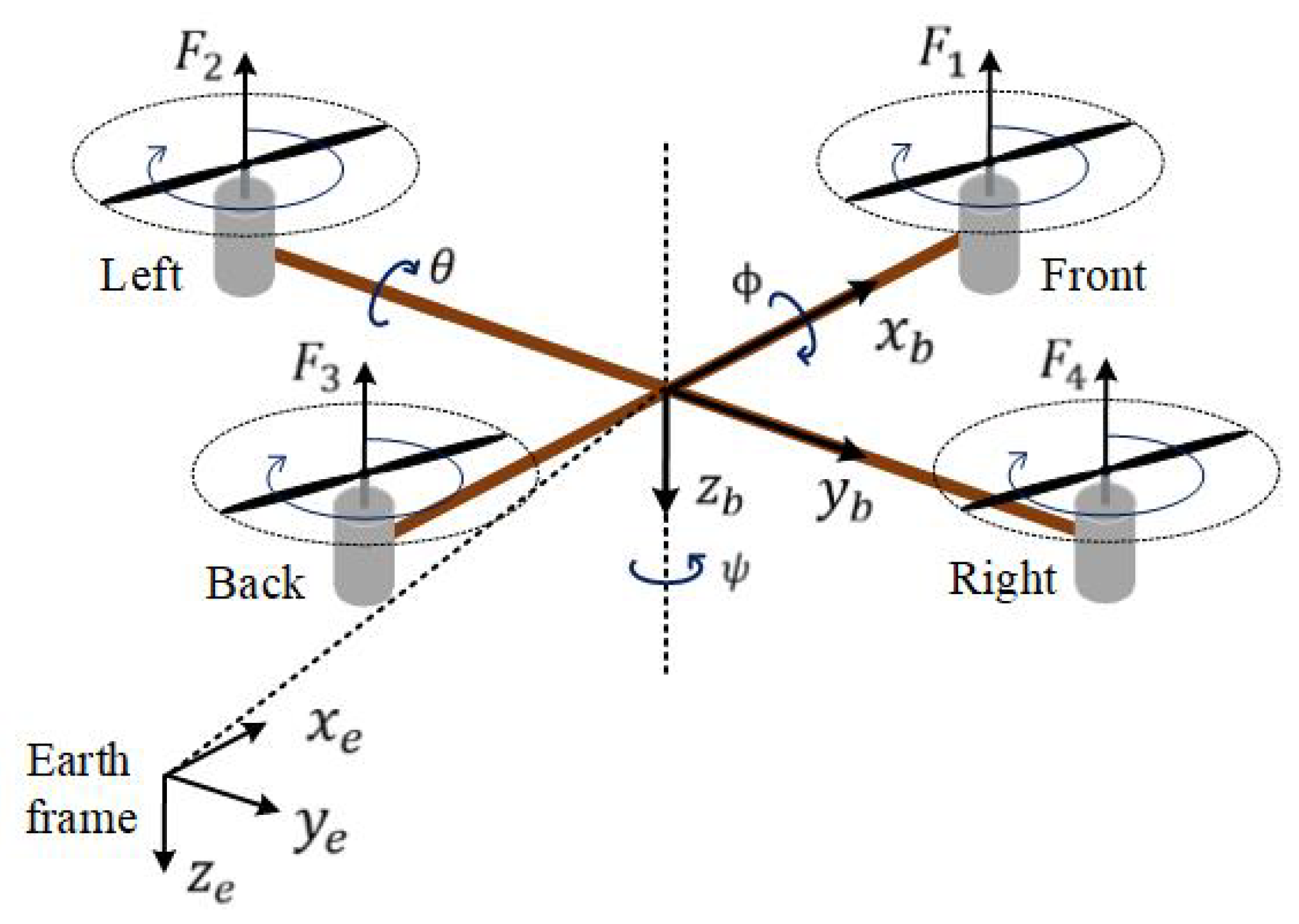
3. System Description and Modeling

The UAV employed in this study was a quadcopter with a symmetric rigid structure and driven by four motors, as shown in Figure 2. For the quadcopter, the pitch angle, varied in accordance with the quadcopter’s longitudinal motion, is controlled by adjusting the front and rear propellers’ velocities, which generate the force $F_1$ and $F_3$. Meanwhile, its lateral displacement is governed by the roll angle, which is controlled through the right and left rotors’ speeds, resulting in the forces $F_2$ and $F_4$. Finally, the yaw angle, associated with the UAV yaw motion, is regulated by the difference between torques generated by these pairs of rotors. In this work, we focused on the attitude tracking control, and thus, only the quadcopter orientation is considered here. The torques acting on the quadcopter include the thrust forces $\tau$, the gyroscopic torques caused by the rotation of the quadcopter’s rigid body ${\tau }_b$ and of four propellers ${\tau }_p$, as well as the torque due to aerodynamic friction ${\tau }_a$. Here, the propellers’ gyroscopic effects and the drag from air resistance are considered external disturbances.

3.1. Kinematics

As shown in the configuration in Figure 2, an earth frame, $\{x_e,y_e,z_e\}$, is fixed at the ground and a body frame, $\{x_b,y_b,z_b\}$, is attached to the CoG of the quadcopter, both with the z axis pointing downward. The position of the UAV’s mass center in the earth frame is defined by a vector $P={(x,y,z)}^T$. The UAV orientation is represented by angles ${(\varphi ,\theta ,\psi )}^T$, corresponding to roll, pitch, and yaw motion, respectively. For attitude control, these angles are limited as $\varphi \in [-\pi /2,\pi /2],\theta \in [-\pi /2,\pi /2]$ and $\psi \in [-\pi ,\pi ]$. With respect to the earth frame, the orientation of the quadcopter is obtained a rotation transformation resulting from successively rotating around the $x_b,y_b$ and $z_b$ axes, and characterized by an orthonormal rotation matrix R [37]:

$$R=\left[\begin{array}{ccc}{c}_{\psi }{c}_{\theta }& c_{\psi }{s}_{\theta }{s}_{\varphi }-s_{\psi }{c}_{\theta }& c_{\psi }{s}_{\theta }{c}_{\varphi }+s_{\psi }{s}_{\theta }\\ s_{\psi }{c}_{\theta }& s_{\psi }{s}_{\theta }{s}_{\varphi }+c_{\psi }{c}_{\theta }& s_{\psi }{s}_{\theta }{c}_{\varphi }-c_{\psi }{s}_{\theta }\\ -s_{\theta }& c_{\theta }{s}_{\varphi }& c_{\theta }{c}_{\varphi }\end{array}\right],$$

(27)

where $s_x$ and $c_x$ denote $sinx$ and $cosx$, respectively.

Denoting the angular velocity vector of the quadcopter in the body frame as ${\left({\omega }_{\varphi }{\omega }_{\theta }{\omega }_{\psi }\right)}^T$, the rotational kinematics can be obtained as follows [38]:

$${\left[\begin{array}{ccc}\dot{\varphi }& \dot{\theta }& \dot{\psi }\end{array}\right]}^T=W^{-1}{\left[\begin{array}{ccc}{\omega }_{\varphi }& {\omega }_{\theta }& {\omega }_{\psi }\end{array}\right]}^T,$$

(28)

where

$$W^{-1}=\left[\begin{array}{ccc}1& sin\varphi tan\theta & cos\varphi tan\theta \\ 0& cos\varphi & -sin\varphi \\ 0& sin\varphi sec\theta & cos\theta sec\theta \end{array}\right].$$

3.2. Quadcopter Dynamics

From the quadcopter description, the components of torque vector $\tau ={\left[{\tau }_{\varphi }{\tau }_{\theta }{\tau }_{\psi }\right]}^T$, corresponding to rotation in the roll, pitch, and yaw directions, respectively, are calculated as

$${\tau }_{\varphi }=l(F_2-F_4),$$

(29)

$${\tau }_{\theta }=l(-F_1+F_3),$$

(30)

$${\tau }_{\theta }=l(-F_1+F_3),$$

(31)

where l is the distance from each rotor to the CoG, and $\beta$ is the apparent radius for converting the force into the yaw torque.

From (29)–(31), the control inputs are described as:

$$\left[\begin{array}{c}{u}_{\varphi }\\ u_{\theta }\\ u_{\psi }\\ u_z\end{array}\right]=\left[\begin{array}{c}{\tau }_{\varphi }\\ {\tau }_{\theta }\\ {\tau }_{\psi }\\ F\end{array}\right]=\left[\begin{array}{cccc}0& l& 0& -l\\ -l& 0& l& 0\\ -\beta & \beta & -\beta & \beta \\ l& l& l& l\end{array}\right]\left[\begin{array}{c}{F}_1\\ F_2\\ F_3\\ F_4\end{array}\right],$$

(32)

where $u_{\varphi },u_{\theta }$, and $u_{\psi }$ are the roll, pitch, and yaw torques, respectively; $F={\sum }_{n=1}^4{F}_n$ is the lift force, representing the total thrust utilizing from the four motors. As the only attitude of the quadcopter is controlled, $u_z$ is assumed to balance with gravity.

The gyroscopic torque due to the rotation of the symmetric body of the quadcopter is described by [29]:

$${\tau }_b=-SI{\left[\begin{array}{ccc}{\omega }_{\varphi }& {\omega }_{\theta }& {\omega }_{\psi }\end{array}\right]}^T,$$

(33)

where

$$S=\left[\begin{array}{ccc}0& -{\omega }_{\psi }& {\omega }_{\theta }\\ {\omega }_{\psi }& 0& -{\omega }_{\varphi }\\ -{\omega }_{\theta }& {\omega }_{\varphi }& 0\end{array}\right]$$

is a skew-symmetric matrix. As shown in the configuration in Figure 2 with the body frame assigned to the quadcopter, given a mass point $m_i$ with its coordinates $(x_i,y_i,z_i)$ in the body, the quadcopter’s inertia can be obtained as a diagonal matrix:

$$I=\left[\begin{array}{ccc}\sum _i(y_i^2+z_i^2)m_i& 0& 0\\ 0& \sum _i(x_i^2+z_i^2)m_i& 0\\ 0& 0& \sum _i(x_i^2+y_i^2)m_i\end{array}\right]=\left[\begin{array}{ccc}{I}_{xx}& 0& 0\\ 0& I_{yy}& 0\\ 0& 0& I_{zz}\end{array}\right].$$

(34)

Accordingly, Equation (33) can be rewritten as

$${\tau }_b={\left[\begin{array}{ccc}(I_{yy}-I_{zz}){\omega }_{\theta }{\omega }_{\psi }& (I_{zz}-I_{xx}){\omega }_{\varphi }{\omega }_{\psi }& (I_{xx}-I_{yy}){\omega }_{\varphi }{\omega }_{\theta }\end{array}\right]}^T.$$

(35)

The gyroscopic torque due to the rotation of four propellers is determined as [29]:

$${\tau }_p={\left[\begin{array}{ccc}{I}_r{\omega }_r{\omega }_{\theta }& -I_r{\omega }_r{\omega }_{\varphi }& 0\end{array}\right]}^T,$$

(36)

where $I_r$ is the moment of inertia of the rotor of each motor, and ${\omega }_r=-{\omega }_{r1}+{\omega }_{r2}-{\omega }_{r3}+{\omega }_{r4}$ is the residual angular velocity, in which ${\omega }_{r1},\dots ,{\omega }_{r4}$ are the corresponding angular velocities of the propellers.

The air drag torque is calculated as [29]:

$${\tau }_a={\left[\begin{array}{ccc}{k}_{ax}{\omega }_{\theta }^2& k_{ay}{\omega }_{\varphi }^2& k_{az}{\omega }_{\psi }^2\end{array}\right]}^T,$$

(37)

where $k_{ax}$, $k_{ay}$, and $k_{az}$ are aerodynamic friction factors.

The dynamics of the quadcopter in attitude control can then be represented as:

$${\left[\begin{array}{ccc}{\dot{\omega }}_{\varphi }& {\dot{\omega }}_{\theta }& {\dot{\omega }}_{\psi }\end{array}\right]}^T=I^{-1}({\tau }_b+\tau +{\tau }_p-{\tau }_a).$$

(38)

Now, if the propeller gyroscopic and aerodynamic torques are considered as external disturbances, i.e.,

$$d={\left[\begin{array}{ccc}{d}_{\varphi }& d_{\theta }& d_{\psi }\end{array}\right]}^T={\tau }_p-{\tau }_a,$$

(39)

where $d_{\varphi }$, $d_{\theta }$, and $d_{\psi }$ are disturbance components, then substituting (32), (35), and (39) into (38) yields:

$${\dot{\omega }}_{\varphi }=I_{xx}^{-1}\left[(I_{yy}-I_{zz}){\omega }_{\theta }{\omega }_{\psi }+u_{\varphi }+d_{\varphi }\right],$$

(40)

$${\dot{\omega }}_{\theta }=I_{yy}^{-1}\left[(I_{zz}-I_{xx}){\omega }_{\varphi }{\omega }_{\psi }+u_{\theta }+d_{\theta }\right]$$

(41)

$${\dot{\omega }}_{\theta }=I_{yy}^{-1}\left[(I_{zz}-I_{xx}){\omega }_{\varphi }{\omega }_{\psi }+u_{\theta }+d_{\theta }\right].$$

(42)

To express the quadcopter dynamics via the orientation angles, the model can be simplified by considering $[{\omega }_{\varphi },{\omega }_{\theta },{\omega }_{\psi }]\approx [\dot{\varphi },\dot{\theta },\dot{\psi }]$. This approximation is acceptable since a minor model error can be adequately addressed by a good controller. Accordingly, the quadcopter model is obtained as:

$$\ddot{\varphi }=I_{xx}^{-1}\left[(I_{yy}-I_{zz})\dot{\theta }\dot{\psi }+u_{\varphi }+d_{\varphi }\right],$$

(43)

$$\ddot{\theta }=I_{yy}^{-1}\left[(I_{zz}-I_{xx})\dot{\varphi }\dot{\psi }+u_{\theta }+d_{\theta }\right],$$

(44)

$$\ddot{\psi }=I_{zz}^{-1}\left[(I_{xx}-I_{yy})\dot{\varphi }\dot{\theta }+u_{\psi }+d_{\psi }\right].$$

(45)

3.3. Discrete-Time Model

In the discrete-time domain, by considering the difference approximation for first and second derivatives using the forward Euler method, the transformed discrete-time model can be obtained as below:

$$\begin{array}{cc}\hfill \varphi (k+2)& =2\varphi (k+1)-\varphi \left(k\right)+I_{xx}^{-1}(I_{yy}-I_{zz})[\theta (k+1)-\theta \left(k\right)][\psi (k+1)-\psi \left(k\right)]\hfill \\ \hfill & +{\mathsf{\Delta }}_t^2{I}_{xx}^{-1}\left[u_{\varphi }\left(k\right)+d_{\varphi }\left(k\right)\right],\hfill \end{array}$$

(46)

$$\begin{array}{cc}\hfill \theta (k+2)& =2\theta (k+1)-\theta \left(k\right)+I_{yy}^{-1}(I_{zz}-I_{xx})[\varphi (k+1)-\varphi \left(k\right)][\psi (k+1)-\psi \left(k\right)]\hfill \\ \hfill & +{\mathsf{\Delta }}_t^2{I}_{yy}^{-1}\left[u_{\theta }\left(k\right)+d_{\theta }\left(k\right)\right],\hfill \end{array}$$

(47)

$$\begin{array}{cc}\hfill \psi (k+2)& =2\psi (k+1)-\psi \left(k\right)+I_{zz}^{-1}(I_{xx}-I_{yy})[\varphi (k+1)-\varphi \left(k\right)][\theta (k+1)-\theta \left(k\right)]\hfill \\ \hfill & +{\mathsf{\Delta }}_t^2{I}_{zz}^{-1}\left[u_{\psi }\left(k\right)+d_{\psi }\left(k\right)\right].\hfill \end{array}$$

(48)

Now, consider the system state vector $x\left(k\right)={\left[x_1\left(k\right)x_2\left(k\right)\right]}^T$ defined by:

$$x_1\left(k\right)={\left[\begin{array}{ccc}{\varphi }_1\left(k\right)& {\theta }_1\left(k\right)& {\psi }_1\left(k\right)\end{array}\right]}^T={\left[\begin{array}{ccc}\varphi \left(k\right)& \theta \left(k\right)& \psi \left(k\right)\end{array}\right]}^T,$$

(49)

$$x_2\left(k\right)={\left[\begin{array}{ccc}{\varphi }_2\left(k\right)& {\theta }_2\left(k\right)& {\psi }_2\left(k\right)\end{array}\right]}^T={\left[\begin{array}{ccc}\frac{\varphi (k+1)-\varphi \left(k\right)}{{\mathsf{\Delta }}_t}& \frac{\theta (k+1)-\theta \left(k\right)}{{\mathsf{\Delta }}_t}& \frac{\psi (k+1)-\psi \left(k\right)}{{\mathsf{\Delta }}_t}\end{array}\right]}^T.$$

(50)

From (46)–(50), we obtain the UAV state equation in discrete time of the form (1) as:

$$x_1(k+1)=x_1\left(k\right)+{\mathsf{\Delta }}_t{x}_2\left(k\right),$$

(51)

$$x_2(k+1)=f\left(x\left(k\right)\right)+{\mathsf{\Delta }}_{t}B[u\left(k\right)+d\left(k\right)],$$

(52)

where $f\left(x\left(k\right)\right)=x_2\left(k\right)+{\mathsf{\Delta }}_t{I}^{-1}{\tau }_b\left(k\right)$ and $B=I^{-1}$.

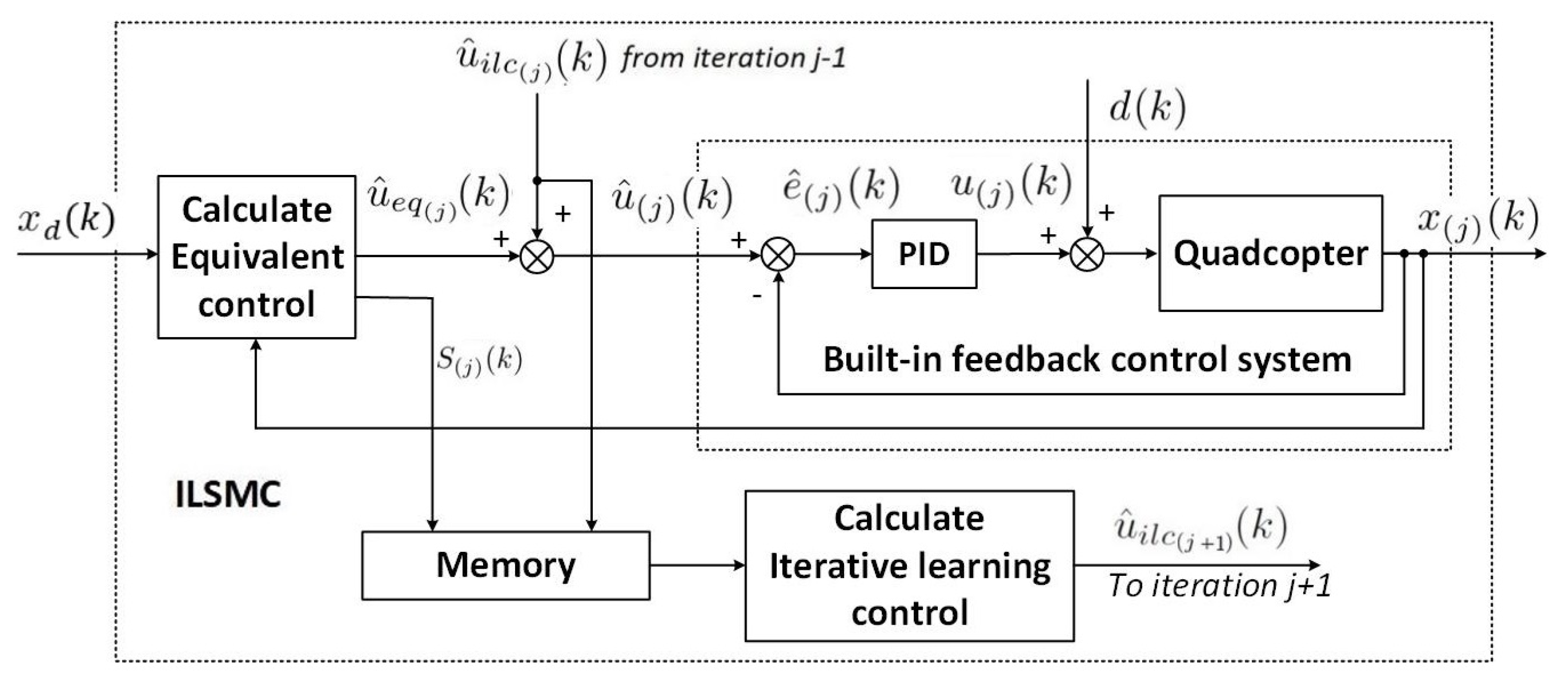
4. Integrated ILSMC for UAV Attitude Control

The proposed ILSMC was then applied to the outer loop of a quadcopter with a built-in PID controller in the inner loop for flight control. Here, the ILSMC is integrated in cascade control to improve the performance of the UAV trajectory tracking in dealing with noise, nonrepeating uncertainties, and disturbances. Figure 3 shows the block diagram of the proposed controller wherein the reference signal of a feedback controller is generated by the ILSMC signal ${\widehat{u}}_{\left(j\right)}\left(k\right)$ at a time instant k.

4.1. Inner-Loop PID Controller

As shown in Figure 3, the output of the quadcopter PID controller is computed as

$$u_{\left(j\right)}\left(k\right)=K_p\circ {\widehat{e}}_{\left(j\right)}\left(k\right)+K_i{\mathsf{\Delta }}_t\circ \sum _{\kappa =1}^k{\widehat{e}}_{\left(j\right)}\left(\kappa \right)+K_d{\mathsf{\Delta }}_t^{-1}\circ [{\widehat{e}}_{\left(j\right)}\left(k\right)-{\widehat{e}}_{\left(j\right)}(k-1)],$$

(53)

where ∘ denotes the elementwise Hadamard product; $K_p={\left[\begin{array}{c}{K}_{p_{\varphi }}{K}_{p_{\theta }}{K}_{p_{\psi }}\end{array}\right]}^T$, $K_i={\left[\begin{array}{c}{K}_{i_{\varphi }}{K}_{i_{\theta }}{K}_{i_{\psi }}\end{array}\right]}^T$, and $K_d={\left[\begin{array}{c}{K}_{d_{\varphi }}{K}_{d_{\theta }}{K}_{d_{\psi }}\end{array}\right]}^T$ are PID control parameters. The error of the PID feedback loop ${\widehat{e}}_{\left(j\right)}\left(k\right)$ is defined as

$${\widehat{e}}_{\left(j\right)}\left(k\right)={\widehat{u}}_{\left(j\right)}\left(k\right)-x_{\left(j\right)}\left(k\right),$$

(54)

where ${\widehat{u}}_{\left(j\right)}\left(k\right)$ is the ILSMC control signal.

Substituting (54) into (53) yields:

$$u_{\left(j\right)}\left(k\right)=D\circ {\widehat{u}}_{\left(j\right)}\left(k\right)+H\left(k\right),$$

(55)

where

$$D=K_p+K_i{\mathsf{\Delta }}_t+K_d/{\mathsf{\Delta }}_t,$$

(56)

$$H\left(k\right)=-D\circ x_{\left(j\right)}\left(k\right)+K_i{\mathsf{\Delta }}_t\circ \sum _{\kappa =1}^{k-1}{\widehat{e}}_{\left(j\right)}\left(\kappa \right)-K_d\circ {\widehat{e}}_{\left(j\right)}(k-1){\mathsf{\Delta }}_t^{-1}.$$

(57)

4.2. Outer-Loop ILSMC

As mentioned above, the proposed ILSMC was then added to the predesigned PID controller for improving the UAV tracking performance. Substituting (55) into (10) yields:

$$\begin{array}{cc}\hfill {\mathsf{\Delta }}_t^{-1}[f\left(x_{\left(j\right)}\left(k\right)\right)+{\mathsf{\Delta }}_{t}B(D\circ {\widehat{u}}_{\left(j\right)}\left(k\right)& +H\left(k\right)+d\left(k\right))-x_{2d}(k+1)\hfill \\ \hfill & +(c{\mathsf{\Delta }}_t-1)e_{2\left(j\right)}\left(k\right)]+\mu {\sigma }_{\left(j\right)}\left(k\right)=0.\hfill \end{array}$$

(58)

The equivalent control of the outer loop is then given by:

$$\begin{array}{cc}\hfill {\widehat{u}}_{e{q}_{\left(j\right)}}\left(k\right)=D^{-1}\circ {\left({\mathsf{\Delta }}_{t}B\right)}^{-1}\{-f\left(x_{\left(j\right)}\left(k\right)\right)& -{\mathsf{\Delta }}_{t}BH\left(k\right)+x_{2d}(k+1)\hfill \\ \hfill & -(c{\mathsf{\Delta }}_t-1)e_{2\left(j\right)}\left(k\right)-{\mathsf{\Delta }}_t\mu {\sigma }_{\left(j\right)}\left(k\right)\}.\hfill \end{array}$$

(59)

In the learning step, the iterative learning term is computed as

$${\widehat{u}}_{il{c}_{\left(j\right)}}\left(k\right)={\widehat{u}}_{il{c}_{(j-1)}}\left(k\right)-D^{-1}\circ {\left({\mathsf{\Delta }}_{t}B\right)}^{-1}\lambda S_{(j-1)}\left(k\right),$$

(60)

where $S_{(j-1)}\left(k\right)$ is obtained from the learning process at a previous iteration $(j-1)$ as per (15).

This finally leads to the integrated iterative learning sliding mode control law (13) for the quadcopter:

$${\widehat{u}}_{\left(j\right)}\left(k\right)={\widehat{u}}_{e{q}_{\left(j\right)}}\left(k\right)+{\widehat{u}}_{il{c}_{\left(j\right)}}\left(k\right).$$

(61)

4.3. Implementation Procedure

In summary, a step-by-step procedure to implement the proposed control scheme is summarized as:

• Step 1: Declare $I_{xx},I_{yy},I_{zz}$, $K_p,K_i,K_d,c,\mu ,\lambda$.
• Step 2: Set $x_d\left(k\right)$, $j=0$, and ${\widehat{u}}_{il{c}_{\left(j\right)}}\left(k\right)=0$.
• Step 3: Compute the ILSMC ${\widehat{u}}_{\left(j\right)}\left(k\right)$ from (61) as a reference to the inner loop.
• Step 4: Compute, from the measured states $x_{\left(j\right)}\left(k\right)$, $e_{\left(j\right)}\left(k\right)$, ${\sigma }_{\left(j\right)}\left(k\right)$, $S_{\left(j\right)}\left(k\right)$, and the selected TPI.
• Step 5: Check if the tracking performance requirement is met to terminate the learning process. Otherwise, proceed to Step 6.
• Step 6: Set $j=j+1$, update ${\widehat{u}}_{il{c}_{\left(j\right)}}\left(k\right)$ from (60), then return to Step 3.

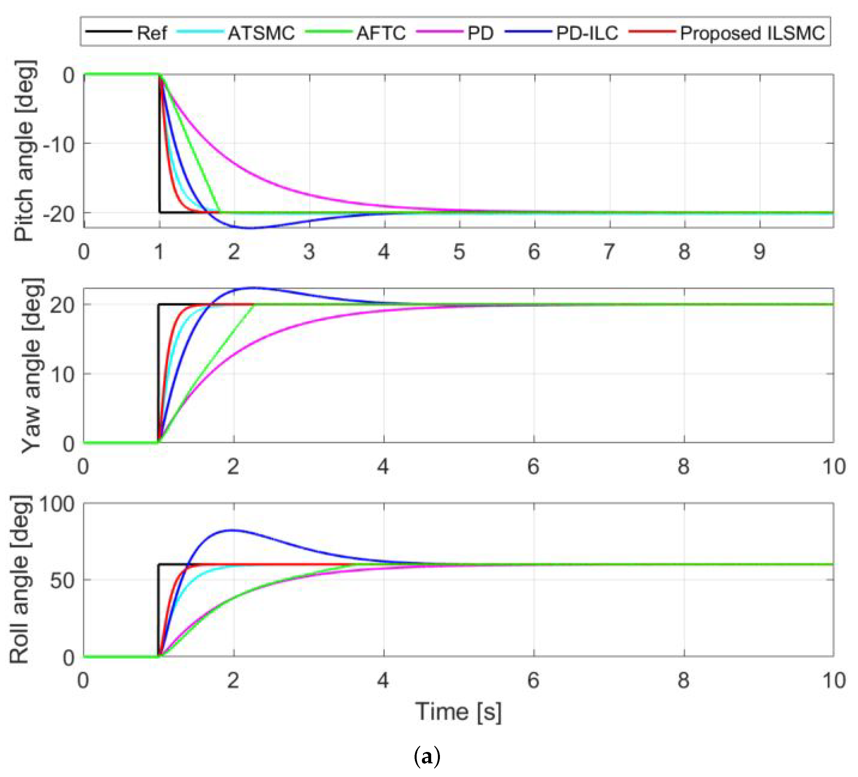
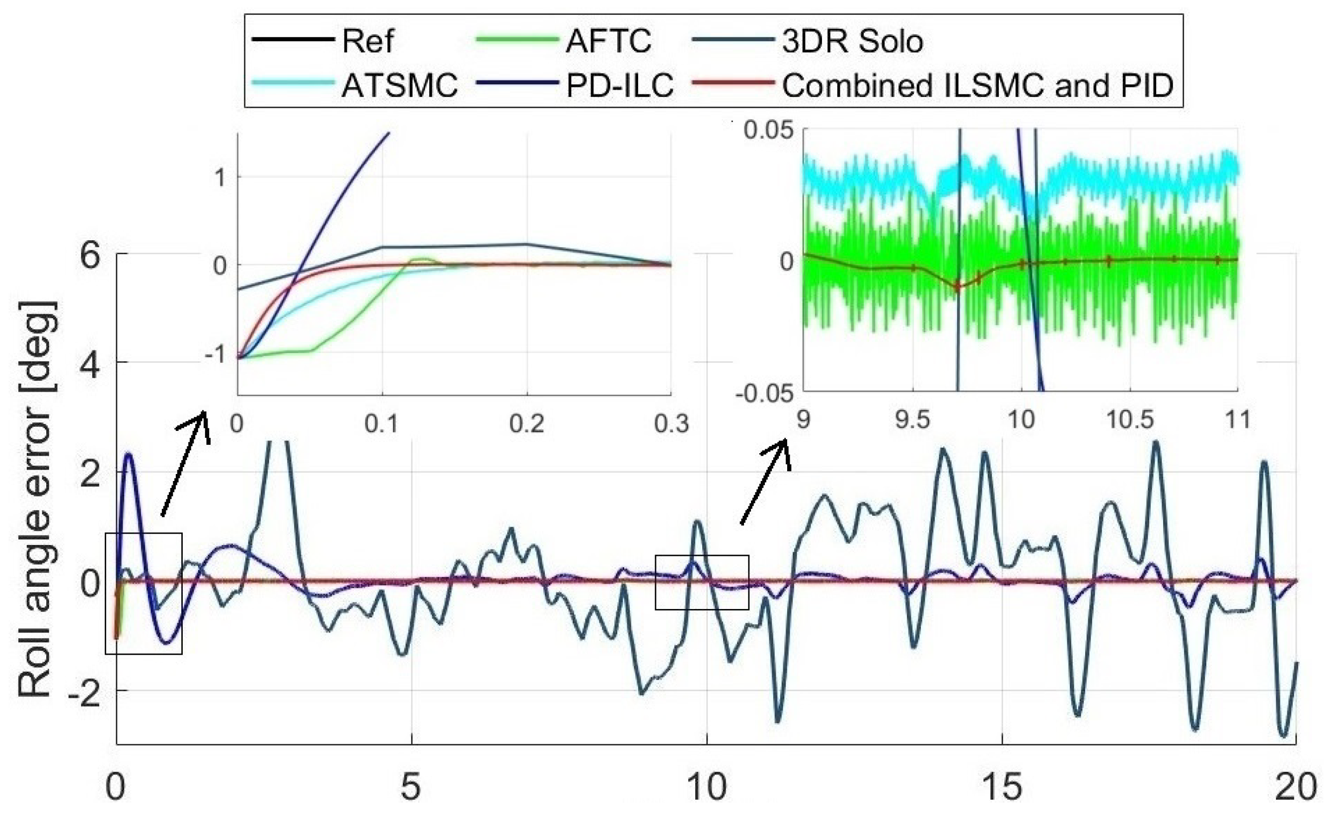
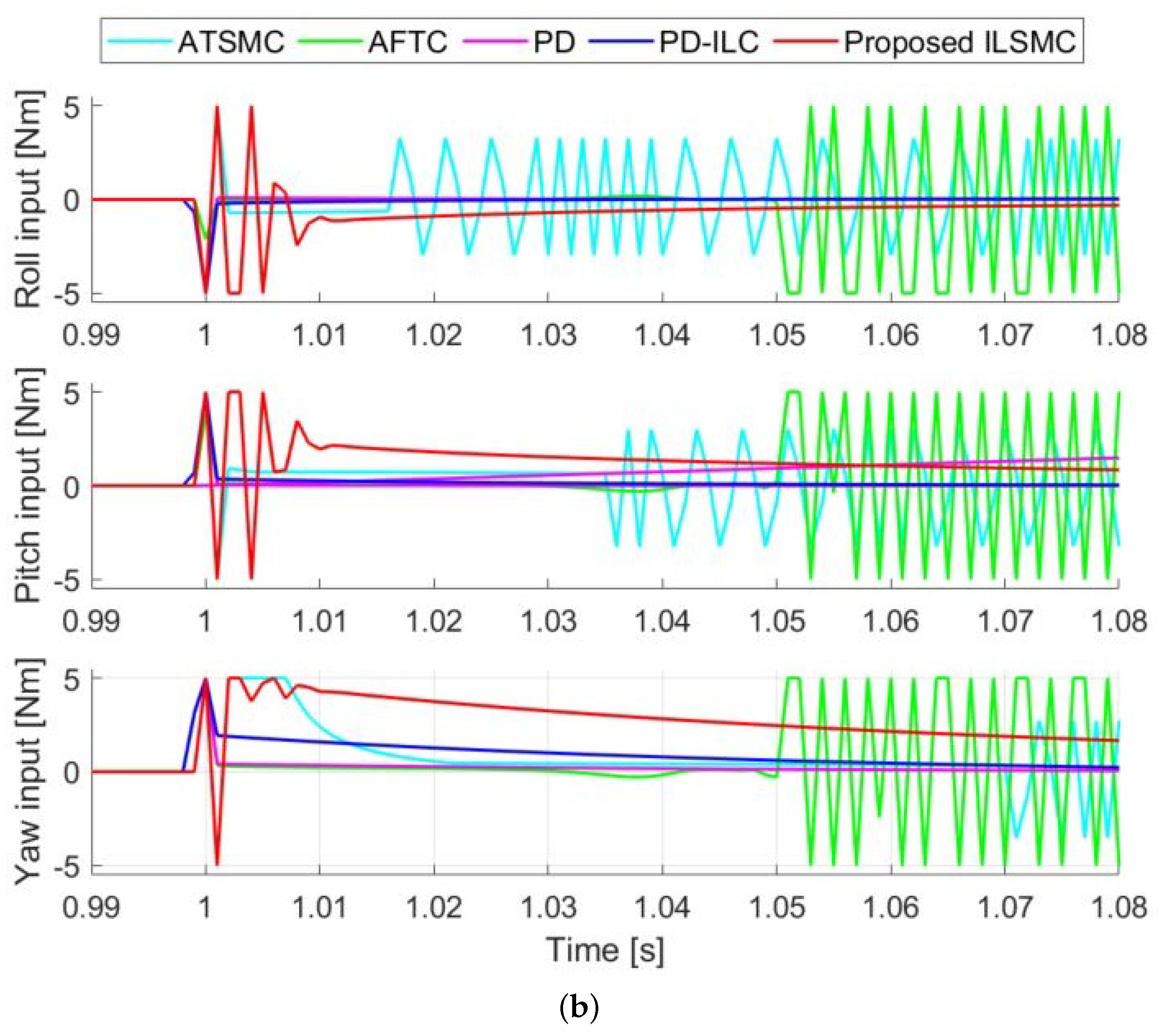
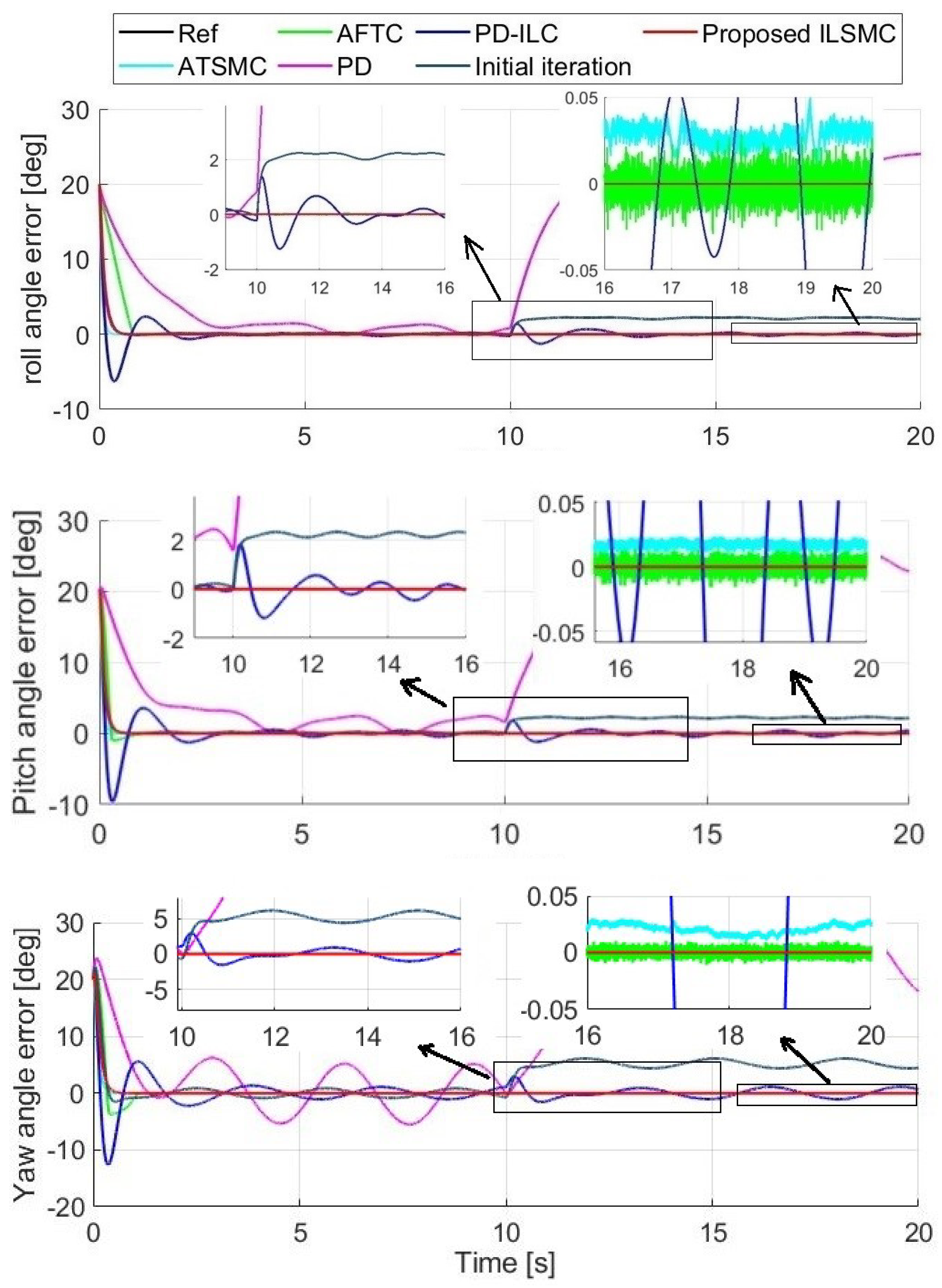
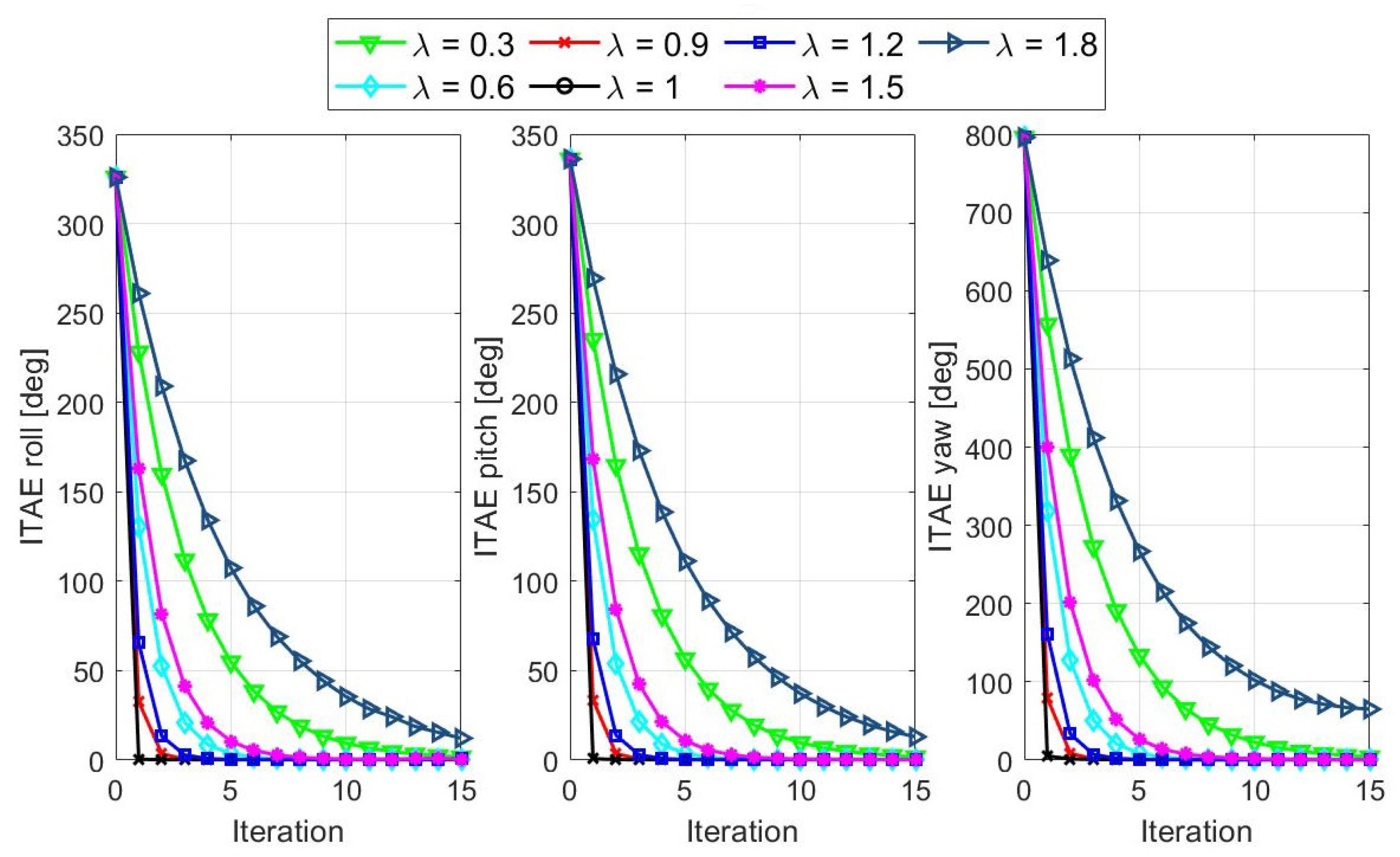
5. Simulation Results

This section provides the simulation results of the proposed ILSMC design. The parameters used for simulation were obtained from the 3DR Solo drone [29], as listed in

Table 1. Parameters of the 3DR Solo drone.

Parameter	Value	Unit
m	$1.5$	kg
l	$0.205$	m
g	$9.81$	m/s${}^2$
$I_{xx}$	$9.1\times {10}^{-3}$	kg m${}^2$
$I_{yy}$	$16.4\times {10}^{-3}$	kg m${}^2$
$I_{zz}$	$24.1\times {10}^{-3}$	kg m${}^2$

. The selected control parameters are described in

Table 2. Control parameters.

Parameter	Value	Parameter	Value
$c_{\varphi }$	50	$\mu$	10
$c_{\theta }$	50	$\lambda$	$0.9$
$c_{\psi }$	20	-	-

. Here, in the learning process, a suitable value for $\lambda$ was chosen to obtain a fast convergence rate, so $S_{\left(j\right)}\left(k\right)$ was driven to zero quickly. In the control phase, coefficients $c_{\varphi }$, $c_{\theta }$, $c_{\psi }$, and $\mu$ were chosen by the desired error dynamics described in (3). Initially, the iterative learning control signal was set to zero, $u_{il{c}_{\left(0\right)}}\left(k\right)=0$, and then updated after each iteration. To evaluate performance of the proposed controller, we compared it with other available techniques including the PD feedback controller, PD-type ILC [19], adaptive twisting sliding mode controller (ATSMC) [29], and adaptive finite-time control scheme (AFTC) [30].

5.1. Step Response in Nominal Conditions

In this section, the performance of the proposed controller is evaluated via the step responses in nominal conditions where disturbances and uncertainties were set to zero. The desired reference attitude angles were set to ${\varphi }_d=-{20}^{\circ }$, ${\theta }_d={20}^{\circ }$, and ${\psi }_d={60}^{\circ }$ at 1 s. The simulation results of the step responses and control signals are shown in Figure 4, in which the black step signal is the desired angle, and responses of ATSMC, AFTC, PD, PD-ILC, and the proposed ILSMC controllers are depicted in cyan, green, magenta, blue, and red, respectively. It can be seen from Figure 4 for all three orientation angles that while ATSMC and AFTC provide some oscillations in the control, and PD presents a slow response, both iterative-learning-based techniques, ILSMC and PD-ILC, exhibit fast responses with zero steady-state error. PDILC, however, incurs a large overshoot, whereas ILSMC is able to maintain the desired dynamics without overshoot owing to the merits of sliding mode control. Notably, the fast response of ILSMC in comparison to ATSMC, AFTC, PD, ILC, and PD is attributed to the choice of $c=\mathrm{diag}(c_{\varphi },c_{\theta },c_{\psi })$ and $\mu$. A faster transient response, however, requires more control efforts that may exceed the physical limits imposed by the motors and power supply for the drone. Moreover, the proposed controller is chattering-free in the steady state.

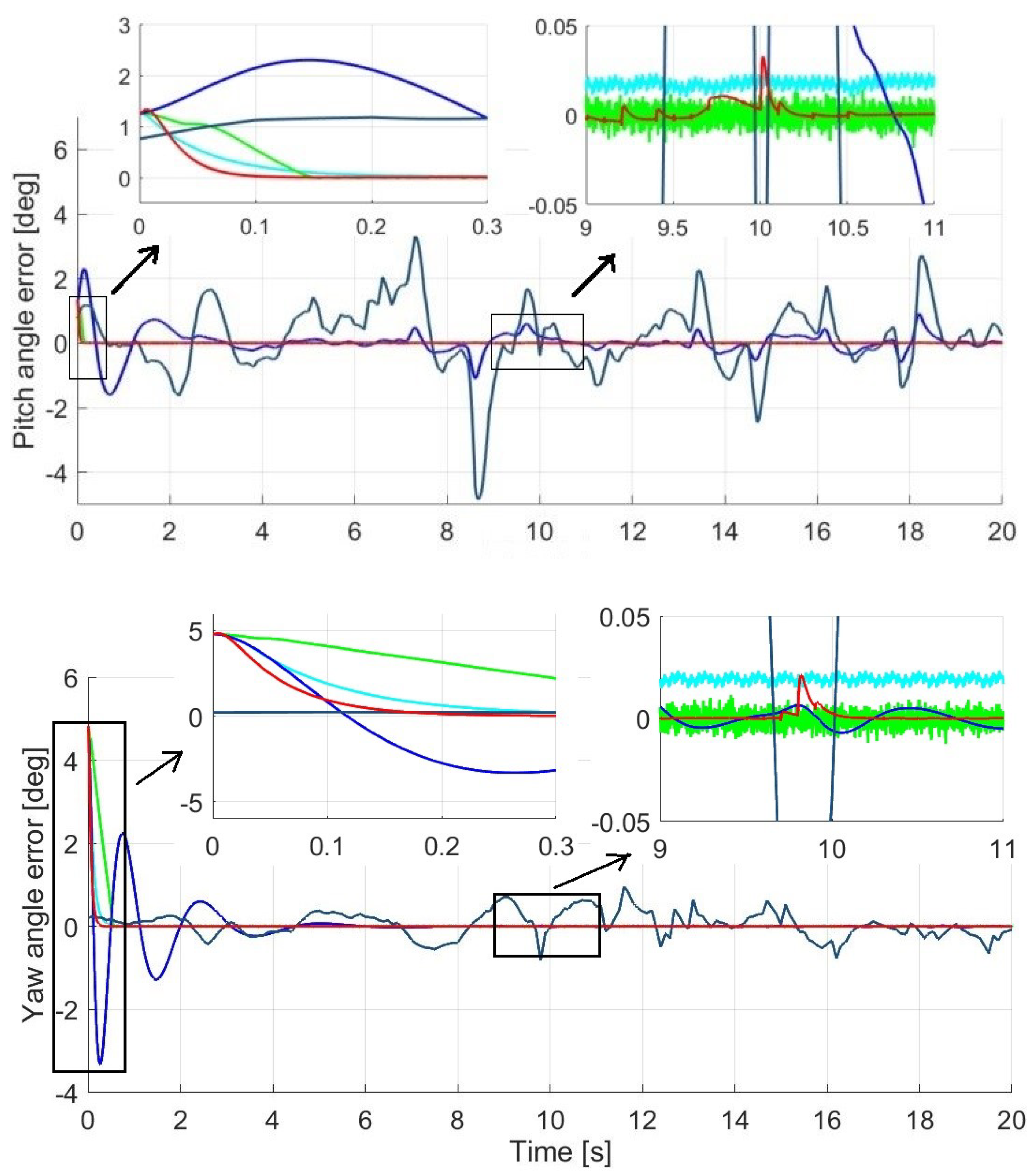
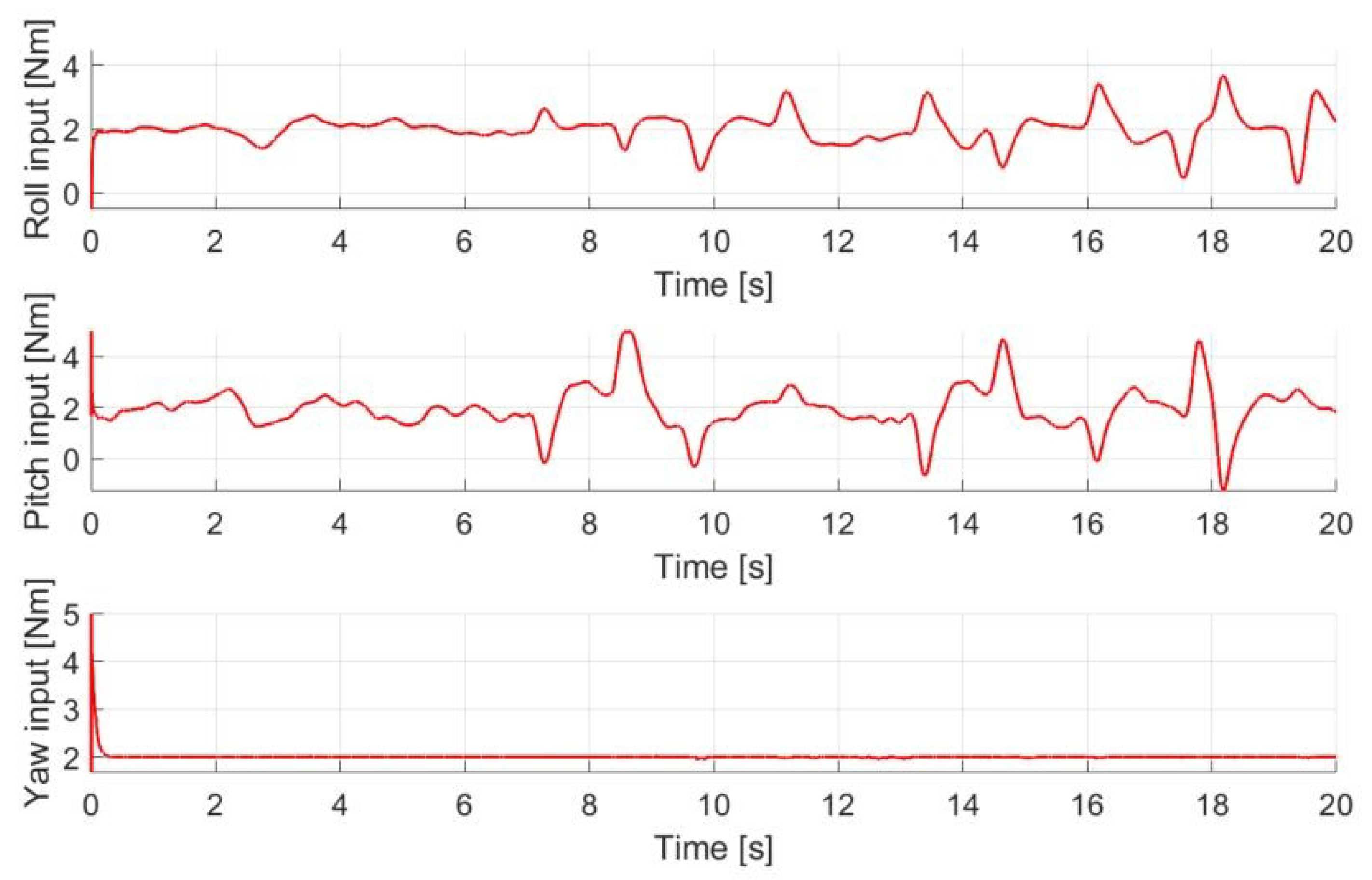
5.2. Trajectory Tracking Performance under Disturbances and Uncertainties

To evaluate the tracking performance of ILSMC with the presence of uncertainties and disturbances caused by load variations, the reference attitude angles in this simulation were set, in degrees, as below:

$$\begin{array}{cc}\hfill {\varphi }_d\left(k\right)& =20-20sin\left(2k\right),\hfill \\ \hfill {\theta }_d\left(k\right)& =20+20sin\left(2k\right),\hfill \\ \hfill {\psi }_d\left(k\right)& =20+60sin\left(2k\right).\hfill \end{array}$$

(62)

For performance evaluation, the system was injected with a disturbance at $t=10$ s whose components were:

$$d_{\varphi }=d_{\theta }=d_{\psi }=-0.2.$$

(63)

Considering 20% loading conditions, the model uncertainties were introduced by setting:

$${\widehat{I}}_{xx}=1.2I_{xx},{\widehat{I}}_{yy}=1.2I_{yy},{\widehat{I}}_{zz}=1.2I_{zz},$$

(64)

where ${\widehat{I}}_{xx},{\widehat{I}}_{yy}$, and ${\widehat{I}}_{zz}$ are the estimation of $I_{xx},I_{yy}$, and $I_{zz}$, respectively.

Figure 5 shows the tracking performance of the attitude angles, while

Table 3. ITAE of UAV attitude control angles.

UAV Angle (degrees)	ATSMC	AFTC	PD	PD-ILC	ILSMC
Roll	$5.03$	$2.03$	$3344.2$	$39.91$	$0.255$
Pitch	$3.87$	$1.40$	$3468.4$	$55.60$	$0.261$
Yaw	$3.47$	$2.42$	$3323.0$	$149.89$	$0.444$

presents the TPI, for which the integral time absolute error (ITAE) is adopted here for all angles. It can be seen that the PD controller cannot cope with disturbances with large tracking errors at $t=10\mathrm{s}$ and high values of ITAE. As with PDILC, it can suppress disturbances but suffers from control overshoot and a noticeable error. Both the ATSMC and AFTC techniques present relatively accurate tracking performance with a small ITAE, between $1.40$ and $5.03$. The proposed ILSMC presents a relatively large tracking error at the first iteration (since $u_{il{c}_{\left(0\right)}}=0$), but owing to the learning ability, the tracking error decreases with increasing iterations by updating the iterative learning control term after each iteration. As the tracking performance is improved significantly, at the last iteration, ILSMC has the smallest ITAE among the considered techniques. Additionally, the absolute error is also the smallest, almost zero in steady state, as shown in the magnified figure, demonstrating the advantage of the proposed ILSMC.

Figure 6 shows the control efforts in the presence of disturbances and uncertainties. It can be seen that its magnitude increases after 10 s, which implies that more energy is required to compensate for the external disturbances. More importantly, the control efforts of ILSMC display oscillation only in the transient state, but no chattering in the steady state, which is beneficial for practical implementation.

To evaluate the effect of the proposed learning mechanism, the ITAE values were computed for ILSMC after each iteration with different values of $\lambda$. The results up to 15 iterations are presented in Figure 7. They indicate that the ITAE of the all three attitude angle errors quickly decreases and converges to zero after several iterations. To induce a fast system sliding mode, a higher rate of convergence must be selected. It can be seen in Figure 7 that this can be obtained when $\lambda$ is close to one. In this work, $\lambda =0.9$ was chosen to achieve the desired control performance.

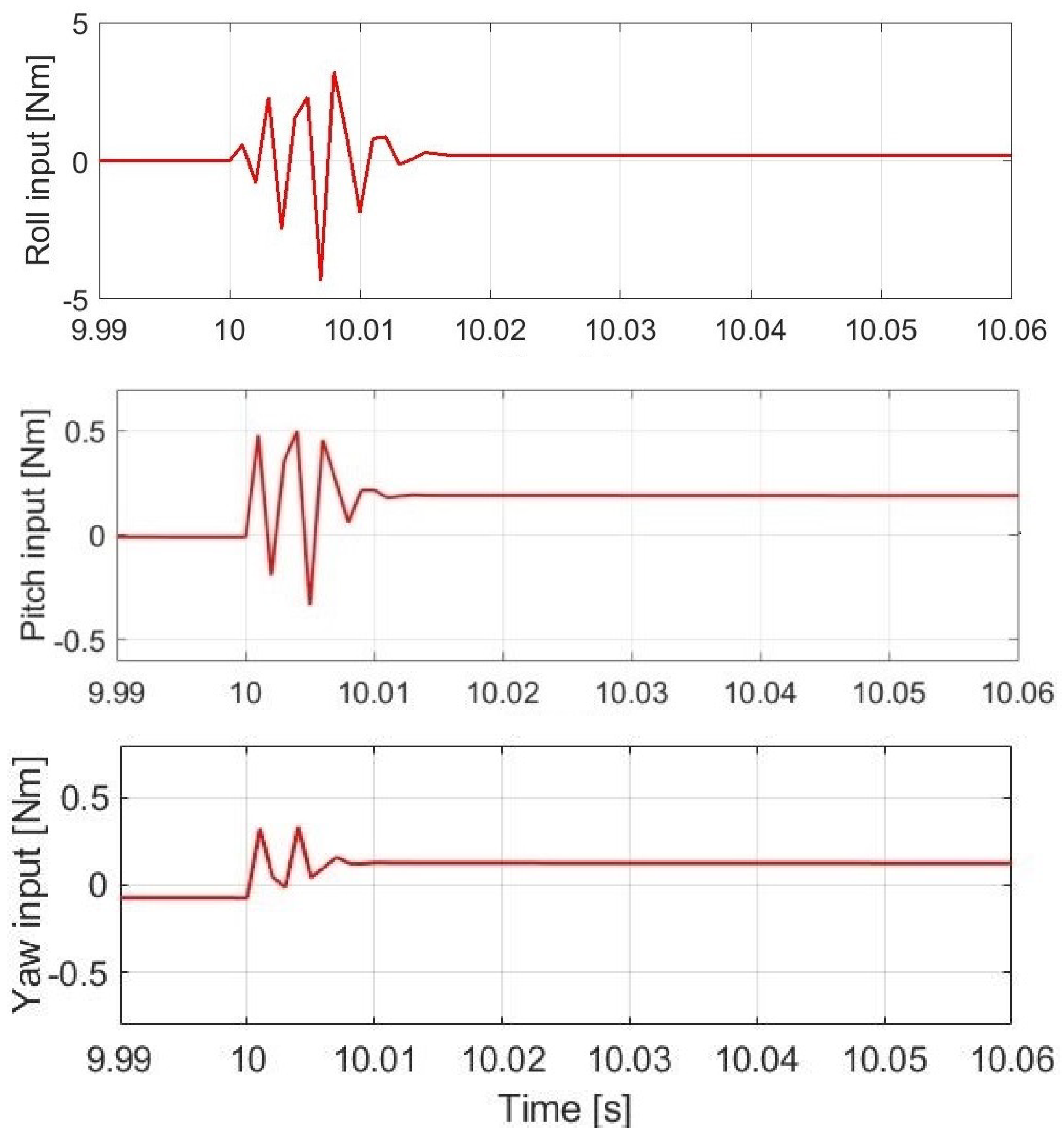
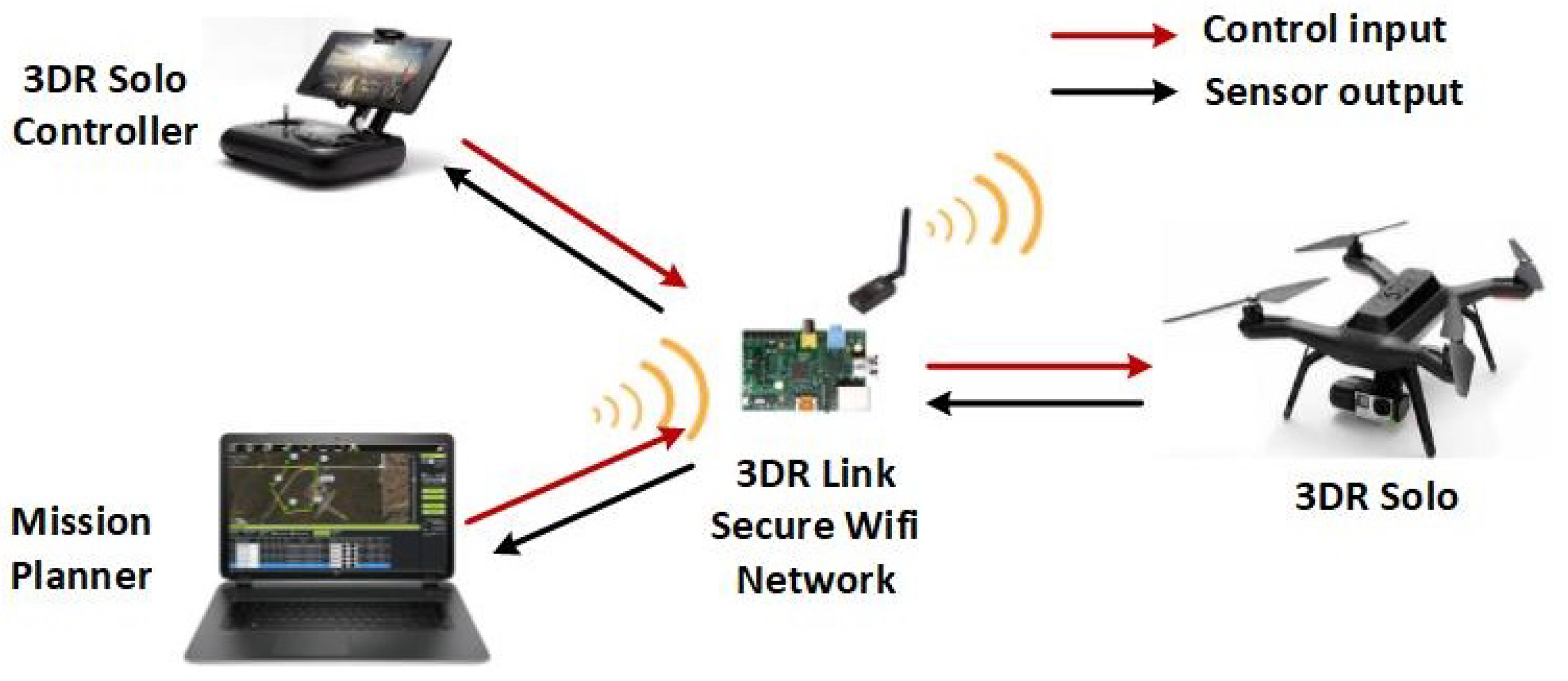
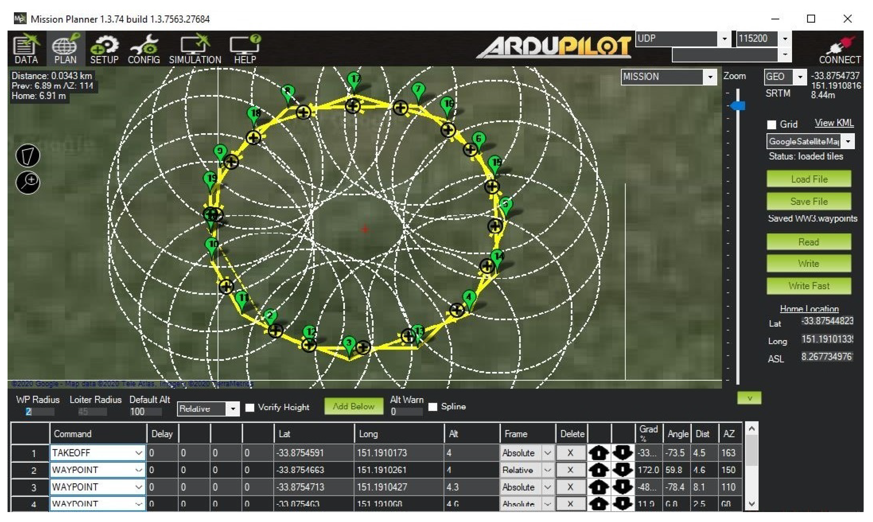
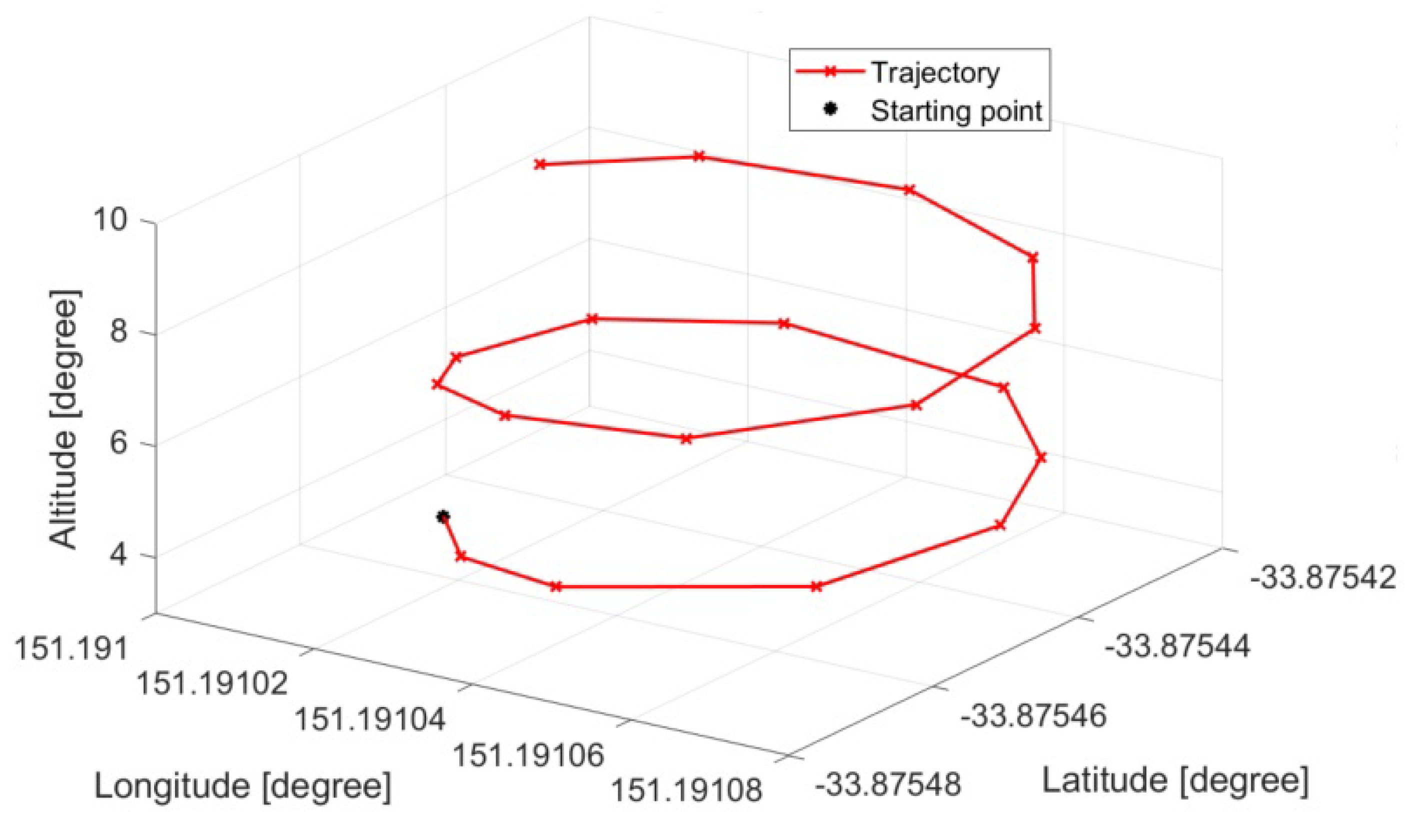
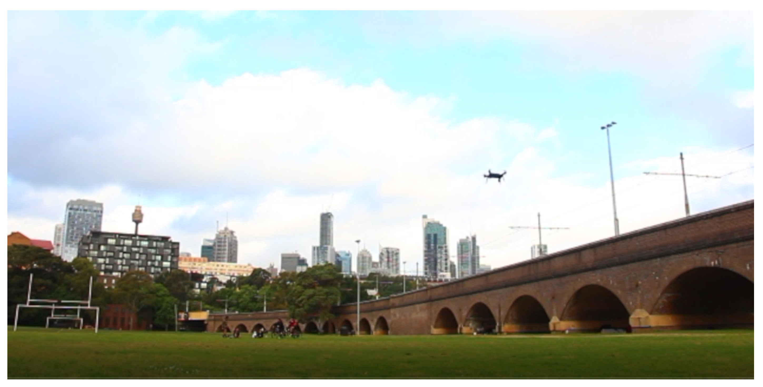
6. Experimental Validation

In this section, we evaluate the performance of the combined ILSMC and PID control algorithm in the trajectory tracking problem for our UAV testbed, in which a built-in PID was already employed.

6.1. Experimental Setup

The setup for the experiments is shown in Figure 8, using a 3DR Solo drone with its parameters described in Table 1 [39]. It consists of two Cortex M4 168 MHz processors used for low-level control and one ARM Cortex A9 processor used for running the Arducopter flight operating system. The drone is equipped with a camera, a laser scanner, and environmental sensors for data acquisition. During the experiments, communication data, including control reference signals and drone sensor outputs, were transmitted to the ground control station via the local network established by the drone system. Mission Planner software was connected to the network to upload the flight plan to the drone and log flight data for analysis. In the experiments, the PID gains were set to their default values implemented in the 3DR Solo. From the desired and actual roll, pitch, and yaw angles, the tracking error was computed.

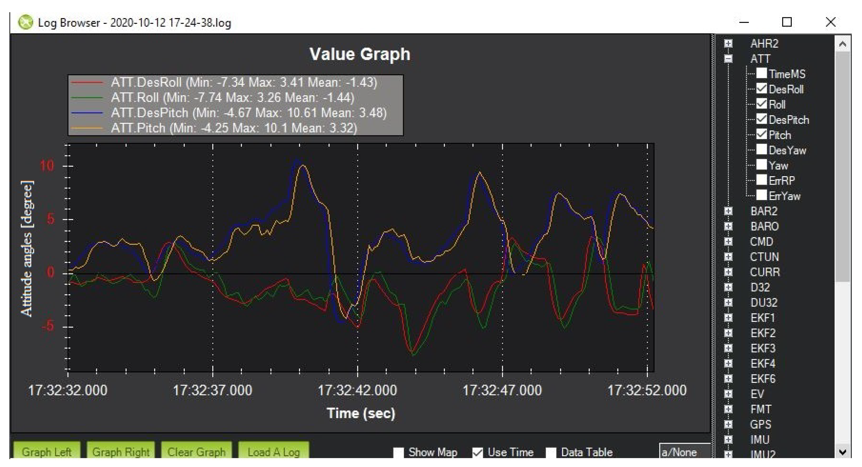
6.2. Real-Time Data Validation Results

The steps for conducting the experiments to validate the trajectory tracking performance of the proposed ILSMC were as follows: First, a trajectory was predefined with a starting point being set at the home position of the drone in an absolute frame of reference, as depicted in Figure 9. After that, the longitude, latitude, and altitude of the waypoints forming the trajectory were imported into Mission Planner, as depicted in Figure 10. Next, those waypoints were uploaded to the 3DR Solo to fly automatically, as shown in Figure 11. Then, the reference and actual attitude angles were logged by Mission Planner, as shown in Figure 12, for comparison. The errors between those angles were used to update the iterative learning term. Finally, the trajectories of the 3DR Solo drone obtained by using the built-in PID controller were compared with the results obtained using ATSMC, AFTC, PD-ILC, and the proposed ILSMC.

The comparison was performed by setting the references obtained from the 3DR Solo drone under similar control settings as in the simulation. Figure 13 shows typical comparison results for the UAV roll, pitch, and yaw responses. It can be seen that the deviation between the reference and the actual roll angle controlled by the built-in PID is relatively high due to disturbances. Advanced techniques can improve the tracking performance in which ILSMC remains the best, as indicated by its smallest tracking error, as can be seen clearly in the insets in the figure. The results obtained confirm the validity and efficiency of the proposed approach.

From the real-time experiments, the recorded control efforts are shown in Figure 14, where the steady-state yaw torque is a constant as the quadcopter was controlled to lift up with a linearly increasing height while performing a circular trajectory during the test.

7. Conclusions

We proposed an effective control technique called ILSMC to address the tracking control problem experienced by quadcopters when subject to disturbances and uncertainties. The control signal consists of an equivalent term to control the system states within the desired sliding surface, and an iterative learning term to drive the system states toward the sliding surface and then remain in the sliding surface despite the presence of uncertainties and disturbances. The iterative learning signal is updated following some iterations to improve the tracking performance by using the data acquired from previous iterations. The simulation results showed, in the case of disturbances and uncertainties, that the iterative learning sliding mode controller presented the smallest tracking errors compared to some other existing control techniques used for quadcopter control. For UAVs with built-in PID controllers, the proposed control scheme can be integrated in a cascade structure to improve the trajectory tracking accuracy and robustness. Field tests were performed, and validation with real-time experimental data was conducted to confirm the advantages of the proposed approach. Our future work will focus on extending the learning mechanism to enable the control of multiple UAVs for real-time formation.

References

1. Grzonka, S.; Grisetti, G.; Burgard, W. A fully autonomous indoor quadrotor. IEEE Trans. Robot. 2012, 28, 90–100. [Google Scholar] [CrossRef] [Green Version]
2. Grisetti, G.; Stachniss, C.; Burgard, W. Non-linear constraint network optimization for efficient map learning. IEEE Trans. Intell. Transp. Syst. 2009, 10, 428–439. [Google Scholar] [CrossRef] [Green Version]
3. Flint, M.; Polycarpou, M.; Fernandez-Gaucherand, E. Cooperative control for multiple autonomous UAV’s searching for targets. In Proceedings of the 41st lEEE Conference on Decision and Control, Las Vegas, NV, USA, 10–13 December 2002. [Google Scholar]
4. Brown, A.; Anderson, D. Trajectory optimization for high-altitude long endurance UAV maritime radar surveillance. IEEE Trans. Aerosp. Electron. Syst. 2020, 56, 2406–2421. [Google Scholar] [CrossRef] [Green Version]
5. Metni, N.; Hamel, T. A UAV for bridge inspection: Visual servoing control law with orientation limits. Autom. Constr. 2007, 17, 3–10. [Google Scholar] [CrossRef]
6. Herwitz, S.R.; Johnson, L.F.; Dunagan, S.E.; Higgins, R.G.; Sullivan, D.V.; Zheng, J.; Lobitz, B.M.; Leung, J.G.; Gallmeyer, B.A.; Aoyagi, M.; et al. Imaging from an unmanned aerial vehicle: Agricultural surveillance and decision support. Comput. Electron. Agric. 2004, 44, 49–61. [Google Scholar] [CrossRef]
7. Choi, Y.C.; Ahn, H.S. Nonlinear control of quadrotor for point tracking: Actual implementation and experimental tests. IEEE/ASME Trans. Mechatron. 2015, 20, 1179–1192. [Google Scholar] [CrossRef]
8. Park, J.; Kim, Y.; Kim, S. Landing site searching and selection algorithm development using vision system and its application to quadrotor. IEEE Trans. Control Syst. Technol. 2015, 23, 488–503. [Google Scholar] [CrossRef]
9. Prasenjit, M.; Steven, W. Direct adaptive feedback linearization for quadrotor control. In Proceedings of the AIAA Guidance, Navigation, and Control Conference, Minneapolis, MN, USA, 13–16 August 2012; American Institute of Aeronautics and Astronautics: Minneapolis, MN, USA, 2012. [Google Scholar]
10. L’afflitto, A.; Anderson, R.B.; Mohammadi, K. An introduction to nonlinear robust control for unmanned quadrotor aircraft. IEEE Control Syst. Mag. 2018, 38, 102–121. [Google Scholar] [CrossRef]
11. Qingtong, W.; Honglin, W.; Qingxian, W.; Mou, C. Backstepping-based attitude control for a quadrotor UAV using nonlinear disturbance observer. In Proceedings of the 2015 34th Chinese Control Conference (CCC), Hangzhou, China, 28–30 July 2015. [Google Scholar]
12. Chincholkar, S.H.; Jiang, W.; Chan, C.-Y. Continuous nonsingular terminal sliding mode control of DC–DC boost converters subject to time-varying disturbances. IEEE Trans. Circuits Syst. II Exp. Briefs 2020, 67, 92–96. [Google Scholar] [CrossRef]
13. Ma, H.; Xiong, Z. Sliding mode control for uncertain discrete-time systems using an adaptive reaching law. IEEE Trans. Circuits Syst. II Exp. Briefs 2021, 68, 722–726. [Google Scholar] [CrossRef]
14. Ali, S.U.; Samar, R.; Shah, M.Z.; Bhatti, A.I.; Munawar, K.; Al-Sggaf, U.M. Lateral guidance and control of UAVs using second-order sliding modes. Aerosp. Sci. Technol. 2016, 49, 88–100. [Google Scholar] [CrossRef]
15. Sankaranarayanan, V.; Mahindrakar, A.D. Control of a class of underactuated mechanical systems using sliding modes. IEEE Trans. Robot. 2009, 25, 459–467. [Google Scholar] [CrossRef]
16. Tian, B.; Yin, L.; Wang, H. Finite-time reentry attitude control based on adaptive multivariable disturbance compensation. IEEE Trans. Ind. Electron. 2015, 62, 5889–5898. [Google Scholar] [CrossRef]
17. Qi, Y.; Zhang, S.; Jiang, F.; Zhou, H.; Tao, D.; Li, X. Siamese local and global networks for robust face tracking. IEEE Trans. Image Process. 2020, 29, 9152–9164. [Google Scholar] [CrossRef] [PubMed]
18. Zhou, M.; Feng, Y.; Xue, C.; Han, F. Deep convolutional neural network based fractional-order terminal sliding-mode control for robotic manipulators. Neurocomputing 2020, 416, 143–151. [Google Scholar] [CrossRef]
19. Bristow, D.A.; Tharayil, M.; Alleyne, A.G. A survey of iterative learning control. IEEE Control Syst. Mag. 2006, 26, 96–114. [Google Scholar]
20. Yu, M.; Li, C. Robust Adaptive Iterative Learning Control for Discrete-Time Nonlinear Systems with Time-Iteration-Varying Parameters. IEEE Trans. Syst. Man Cybern. Syst. 2017, 47, 1737–1745. [Google Scholar] [CrossRef]
21. Uchiyama, M. Formation of high speed motion pattern of mechanical arm by trial. Trans. Soc. Instrum. Control. Eng. 1978, 14, 706–712. [Google Scholar] [CrossRef] [Green Version]
22. Arimoto, S.; Kawamura, S.; Miyazaki, F. Iterative learning control for robot systems. In Proceedings of the IECON, Tokyo, Japan, 22–26 October 1984; pp. 393–398. [Google Scholar]
23. Moore, K.L. Iterative learning control for deterministic systems. In Advances in Industial Control; Springer: London, UK, 1993. [Google Scholar]
24. Tayebi, A.; Abdul, S.; Zaremba, M.B.; Ye, Y. Robust iterative learning control design: Application to a robot manipulator. IEEE/ASME Trans. Mechatron. 2008, 13, 608–613. [Google Scholar] [CrossRef] [Green Version]
25. Mezghani, M.; Roux, G.; Cabassud, M.; Lann, M.V.L.; Dahhou, B.; Casamatta, G. Application of iterative learning control to an exothermic semibatch chemical reactor. IEEE Trans. Control Syst. Technol. 2002, 10, 822–834. [Google Scholar] [CrossRef]
26. Zhu, Q.; Song, F.; Xu, J.; Liu, Y. An internal model based iterative learning control for wafer scanner systems. IEEE/ASME Trans. Mechatron. 2019, 24, 2073–2084. [Google Scholar] [CrossRef]
27. Nikooienejad, N.; Maroufi, M.; Moheimani, R. Iterative learning control for video-rate atomic force microscopy. IEEE/ASME Trans. Mechatron. 2021, 26, 2127–2138. [Google Scholar] [CrossRef]
28. Madani, T.; Benallegue, A. Adaptive control via backstepping technique and neural networks of a quadrotor helicopter. IFAC Proc. Vol. 2008, 41, 6513–6518. [Google Scholar] [CrossRef] [Green Version]
29. Hoang, V.T.; Phung, M.D.; Ha, Q.P. Adaptive twisting sliding mode control for quadrotor unmanned aerial vehicles. In Proceedings of the 2017 Asian Control Conference (ASCC 2017), Gold Coast, Australia, 17–20 December 2017; pp. 671–676. [Google Scholar]
30. Tian, B.; Lu, H.; Zuo, Z.; Zong, Q. Adaptive finite-time attitude tracking of quadrotors with experiments and comparisons. IEEE Trans. Ind. Electron. 2019, 66, 9428–9438. [Google Scholar] [CrossRef]
31. He, X.; Guo, D.; Leang, K.K. Repetitive control design and implementation for periodic motion tracking in aerial robots. In Proceedings of the 2017 American Control Conference (ACC), Seattle, WA, USA, 24–26 May 2017; pp. 5101–5108. [Google Scholar]
32. Dong, J.; He, B. Novel fuzzy PID-type iterative learning control for quadrotor UAV. Sensors 2019, 19, 24. [Google Scholar] [CrossRef] [PubMed] [Green Version]
33. Adlakha, R.; Zheng, M. An Optimization-Based Iterative Learning Control Design Method for UAV’s Trajectory Tracking. In Proceedings of the 2020 American Control Conference (ACC), Denver, CO, USA, 1–3 July 2020; IEEE: Piscataway, NJ, USA, 2020; pp. 1353–1359. [Google Scholar]
34. Chen, Y.; Moore, K.L. Harnessing the nonrepetitiveness in iterative learning control. In Proceedings of the 41st IEEE Conference on Decision and Control, Las Vegas, NV, USA, 10–13 December 2002; IEEE: Piscataway, NJ, USA, 2002; Volume 3, pp. 3350–3355. [Google Scholar]
35. Sarpturk, S.Z.; Istefanopulos, Y.; Kaynak, O. On the stability of discrete-time sliding mode control systems. IEEE Trans. Autom. Control 1987, 32, 930–932. [Google Scholar] [CrossRef]
36. Norrlöf, M.; Gunnarsson, S. Time and frequency domain convergence properties in iterative learning control. Int. J. Control 2002, 75, 1114–1126. [Google Scholar] [CrossRef]
37. Guilherme, V.R.; Manuel, G.O.; Francisco, R.R. An integral predictive/nonlinear H control structure for a quadrotor helicopter. Automatica 2010, 46, 29–39. [Google Scholar]
38. Craig, J.J. Introduction to Robotics—Mechanics and Control, 2nd ed.; Addison-Wesley Publishing Company, Inc.: Reading, MA, USA, 1989. [Google Scholar]
39. Hoang, V.T.; Phung, M.D.; Dinh, T.H.; Ha, Q.P. System architecture for real-time surface inspection using multiple UAVs. IEEE Sens. J. 2020, 40, 4430–4441. [Google Scholar] [CrossRef] [Green Version]
Figure 1. Basic structure of ILC.
Electronics 10 02474 g001
Figure 2. Configuration of a quadcopter.
Electronics 10 02474 g002
Figure 3. ILSMC in a cascade PID-controlled quadcopter.
Electronics 10 02474 g003
Figure 4. Step response in nominal conditions: (a) step response and (b) control effort.
Electronics 10 02474 g004aElectronics 10 02474 g004b
Figure 5. Performance in the presence of disturbances and uncertainties.
Electronics 10 02474 g005
Figure 6. Control efforts in the presence of disturbances and uncertainties.
Electronics 10 02474 g006
Figure 7. ITAEs of the tracking errors after each iteration.
Electronics 10 02474 g007
Figure 8. System architecture.
Electronics 10 02474 g008
Figure 9. Predefined trajectory.
Electronics 10 02474 g009
Figure 10. Imported trajectory.
Electronics 10 02474 g010
Figure 11. Flying 3DR Solo drone.
Electronics 10 02474 g011
Figure 12. Logged flight data.
Electronics 10 02474 g012
Figure 13. Tracking performance with real-time data.
Electronics 10 02474 g013aElectronics 10 02474 g013b
Figure 14. Control efforts with real-time data.
Electronics 10 02474 g014