Lung Segmentation and Characterization in COVID-19 Patients for Assessing Pulmonary Thromboembolism: An Approach Based on Deep Learning and Radiomics

Abstract

The COVID-19 pandemic is inevitably changing the world in a dramatic way, and the role of computed tomography (CT) scans can be pivotal for the prognosis of COVID-19 patients. Since the start of the pandemic, great care has been given to the relationship between interstitial pneumonia caused by the infection and the onset of thromboembolic phenomena. In this preliminary study, we collected n = 20 CT scans from the Polyclinic of Bari, all from patients positive with COVID-19, nine of which developed pulmonary thromboembolism (PTE). For eight CT scans, we obtained masks of the lesions caused by the infection, annotated by expert radiologists; whereas for the other four CT scans, we obtained masks of the lungs (including both healthy parenchyma and lesions). We developed a deep learning-based segmentation model that utilizes convolutional neural networks (CNNs) in order to accurately segment the lung and lesions. By considering the images from publicly available datasets, we also realized a training set composed of 32 CT scans and a validation set of 10 CT scans. The results obtained from the segmentation task are promising, allowing to reach a Dice coefficient higher than 97%, posing the basis for analysis concerning the assessment of PTE onset. We characterized the segmented region in order to individuate radiomic features that can be useful for the prognosis of PTE. Out of 919 extracted radiomic features, we found that 109 present different distributions according to the Mann–Whitney U test with corrected p-values less than 0.01. Lastly, nine uncorrelated features were retained that can be exploited to realize a prognostic signature.

1. Introduction

Since the beginning of the COVID-19 pandemic, researchers have focused on the association between interstitial pneumonia related to the infection and onset of thromboembolic phenomena. In fact, several researchers have found that the clinical aggravations of some patients are correlated to an increase in some laboratory indices, such as D-dimers and fibrinogen, and to the finding of pulmonary embolism (PE) or pulmonary thromboembolism (PTE) detectable with a dedicated computed tomography angiography (CTA) study [1,2,3]. Therefore, the onset of PTE in COVID-19 patients is considered a prognostically unfavorable event that requires prompt treatment with low molecular weight heparin or other anticoagulants [4]. Other researchers have proposed elaborations based on neural topologies in case series of COVID-19 patients in an attempt to provide alternative diagnostic screening tools to the nasopharyngeal swab. The latter still represents the diagnostic gold standard, even if it is expensive, with long sample processing times [5].

Prior to the start of the pandemic, the possibility to detect PTE from CT scans was already considered in some studies [6,7,8,9,10,11]. Cobelli et al. performed a comparison between the CT with and without contrast medium. Exploiting the supervision of an expert radiologist, the authors concluded that in 21 out of 51 examined cases, it was possible to detect the embolus in the unenhanced scan [6]. Mohamed et al. compared the diagnosis of pulmonary embolism from unenhanced CT and CTA scans, by determining the sensitivity and specificity of direct and indirect signs from the latter ones [8]. Sun et al. evaluated the detection of pulmonary embolisms on non-contrast CTs, which were reviewed by two radiologists. Subsequently, a third radiologist performed a final validation. The authors concluded that the non-contrast CTs were not sensitive enough to detect the PE [9]. Tourassi et al. created a computer-aided diagnosis system, based on artificial neural networks, to predict PE from ventilation-perfusion scans and chest radiographs. Their model outperformed physicians’ predictions [10]. Thus, the CTA scan is the election method for diagnosing PTE. Some researchers opted to employ CT scans, but the results were not always satisfactory.

Several recent studies addressed the task of lung parenchyma and lesion segmentation from CT scans in COVID-19 patients [12,13,14,15,16,17,18,19,20,21,22]. Wu et al. proposed a joint classification and segmentation (JCS) system in order to address the issue of performing real-time and explainable COVID-19 diagnosis from CT scans [12]. Akbari et al. developed a method for COVID-19 lesion segmentation from CT images based on active contour models [13]. Cao et al. exploited a convolutional neural network (CNN) based on the U-Net architecture for illustrating the potential of deep learning-based quantitative CT scans for providing an objective assessment of pulmonary involvement and therapy response in COVID-19 [14]. Rajinikanth et al. developed a method that relies on the firefly algorithm and multi-thresholding based on Shannon entropy to enhance the pneumonia lesion. Finally, the Markov random field segmentation is exploited to extract the lesions with higher accuracy. According to the authors, the proposed work obtained a mean accuracy higher than 92% for COVID-19 lesion segmentation [15]. Rajinikanth et al. also proposed an image-assisted system to extract COVID-19 infected sections from lung CT scans in coronal view. The approach considered by the authors incorporates the following steps: thresholding to extract the lung region; image enhancement exploiting harmony search optimization and Otsu thresholding; image segmentation and region of interest (ROI) extraction from the binary image to compute the level of severity [16]. Ter-Sarkisov et al. proposed a one-shot model by exploiting Mask R-CNN [23] functionalities for the COVID-19 classification and lesion segmentation in chest CT scans utilizing the affinity between lesion mask features [17]. Zhao et al. built an open-source dataset composed of 349 COVID-19 CT images, coming from 216 patients, and 463 non-COVID-19 CT images. They also performed experimental studies for developing diagnostic methods based on multi-task learning and self-supervised learning, achieving an F1-score of 90%, an AUC of 98% and an accuracy of 89% [18]. Wang et al. presented their experience in building and deploying an AI system that automatically analyses CT images and provides the probability of infection to rapidly detect COVID-19 pneumonia. By exploiting 1136 training samples (723 were positive for COVID-19) from five hospitals, the authors were able to achieve sensitivity of 97.4% and specificity of 92.2% on the test dataset [19]. Oulefki et al. realized an automatic COVID-19 lung infected region segmentation and measurement approach from CT scan images. The automatic tool proposed by the authors, compared to the state of the art segmentation approaches, i.e., GraphCut, Medical Image Segmentation (MIS), and Watershed, showed better results with an accuracy of 98% [20]. Zheng, Wang et al. proposed a deep learning-based method for COVID-19 detection from chest CT scans, exploiting weak annotations. The lung region was segmented with a pre-trained U-Net. Then the segmented 3D lung region was fed into a 3D deep neural network to predict the probability of COVID-19 infection. The algorithm allowed to obtain an accuracy of 90.1% [21,22].

In this study, we characterized the lung parenchyma and lesions of COVID-19 patients with respect to the onset of PTE. In order to realize this task, accurate segmentation of these ROIs is required. Contrarily to healthy lung parenchyma segmentation, which can be obtained with thresholding, the segmentation of the lesions caused by interstitial pneumonia is not an easy task, since the lesions may be confused with surrounding tissues and vessels. We trained both a healthy lung parenchyma model and a lesion model in order to correctly segment all of the lungs from COVID-19 patients. The first part of the study posed the basis for further analysis on the segmented region, which may be used to establish a relationship between lesions and the onset of PTE. In the second part of the study, we selected different slices from each CT scan, and we extracted features in these regions. These radiomic features were used for characterizing lungs in PTE and non-PTE patients. To the best of our knowledge, no other author has considered the problem of performing statistical analysis of radiomic features from lung and lesion regions with respect to the onset of PTE in COVID-19 patients.

The rest of the paper is structured as follows: in Section 2, we present both the publicly available datasets and the local cohort of the Polyclinic of Bari, concerning CT scans with related annotations for lungs and lesions. In  Section 3, the methods employed to perform the study are described, which involve both deep learning-based semantic segmentation architectures, detailed in Section 3.1, and the radiomics pipeline, introduced in Section 3.2. Mathematical details of the radiomics features considered are available in Appendix A. In Section 4, the obtained results are shown, whereas their discussion is presented in Section 5. Lastly, Section 6 portrays conclusions and future works.

2. Materials

The study considers 20 CT scans of patients positive with COVID-19 from the Polyclinic of Bari. Nine of these patients developed PTE. CT acquisition parameters were the following: slice thickness 0.6 mm, tube voltage 120 kVp, rotation time 0.33 s, pitch 1.2, and acquisition time 2.94 s. Images were reconstructed with a slice thickness of 1 mm in mediastinal and lung settings. Expert radiologists provided COVID-19 lung lesions (8 CT scans) and lung parenchyma (4 CT scans) annotations.

Publicly available datasets have also been considered for this work. Jun et al. provided a collection of 20 CT scans from COVID-19 patients with annotations of the left lung, right lung, and lesions [24]. Two datasets are available at MedSeg (http://medicalsegmentation.com/covid19/, accessed on 8 October 2021). The first consists of 100 axial CT slices, coming from openly accessible JPG images of more than 40 patients, whereas the latter is composed of 9 volumetric CTs taken from Radiopaedia (https://radiopaedia.org/, accessed on 8 October 2021). It should kindly be noted that Radiopaedia images have already been considered in the dataset by Jun et al. [24]. Zaffino et al. described a procedure for performing segmentation of CT images in COVID-19 patients by employing unsupervised learning techniques [25]. The authors realized a publicly available dataset comprised of 50 CT scans with related annotations for healthy lungs, ground-glass opacity (GGO), lung consolidation (LC), and denser tissues. We also deemed a dataset of patients with other lung ailments, VESSEL12 (https://vessel12.grand-challenge.org/, accessed on 8 October 2021), a challenge organized in conjunction with the IEEE International Symposium on Biomedical Imaging (ISBI 2012), held in Barcelona, Spain, from 2 to 5 May, 2012.

The summary of considered datasets is reported in

Table 1. Dataset considered for this study. A stands for air, LP stands for lung parenchyma, LL stands for lung lesions, LC stands for lung consolidation, GGO stands for ground-glass opacity, and DT represents dense tissues.

Dataset	Acronym	Sample	Disease	Annotation
Jun et al. [24]	D1	20 CT	COVID-19	LP, LL
VESSEL12	D2	20 CT	Other lung diseases	LP
Ours	D3	20 CT	COVID-19	LP, GGO, LC
Zaffino et al. [25]	D4	50 CT	COVID-19	A, LP, GGO, LC, DT

, whereas example images are illustrated in Figure 1. The materials herein presented have been exploited for the analysis described in the following section of this paper.

3. Methods

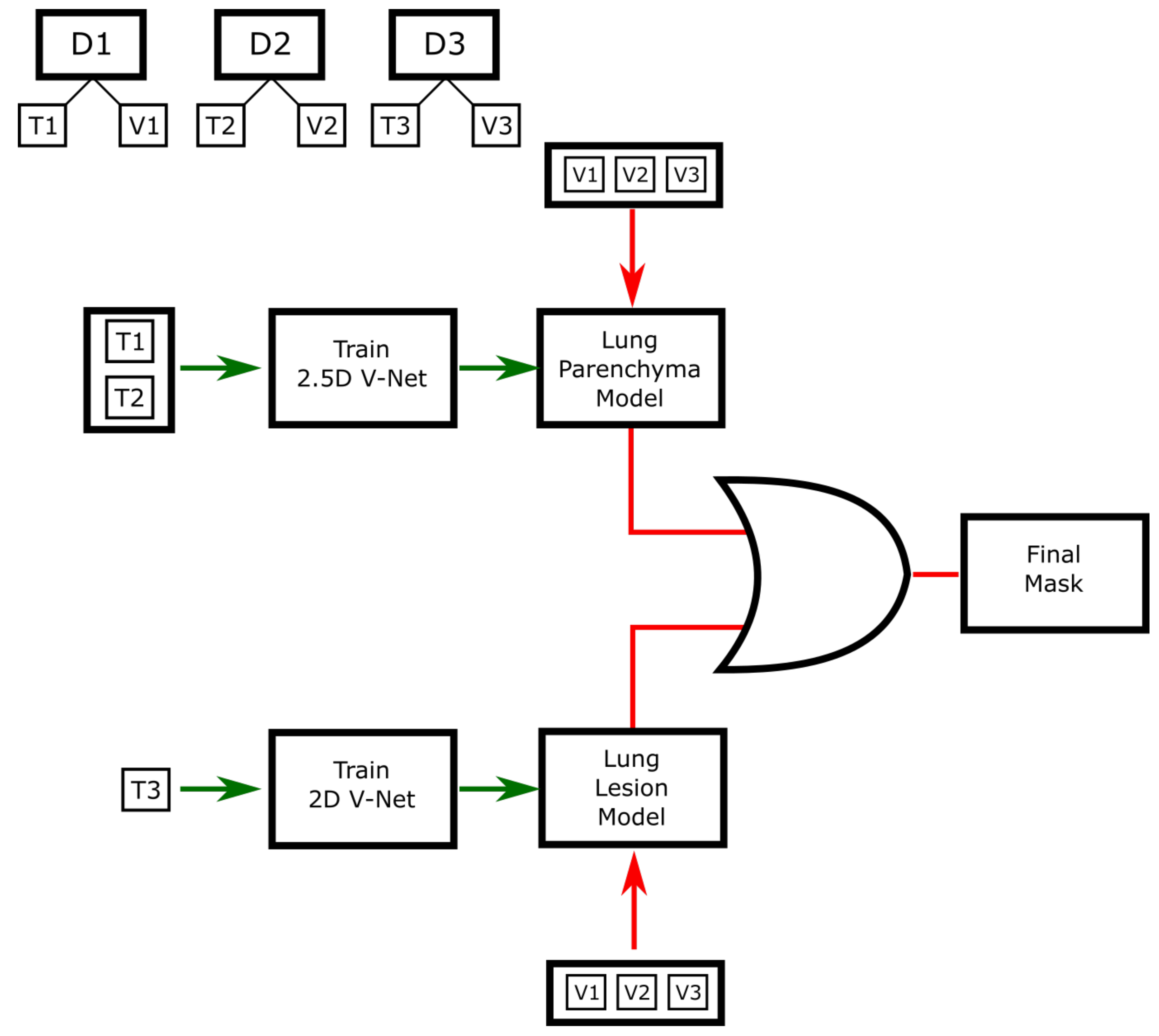
3.1. Semantic Segmentation

Deep learning methodologies show potential in being widely used for medical image analysis tasks due to the accuracy they offer. Deep learning denotes the exploitation of computational models composed of multiple layers of abstraction, which allow obtaining hierarchical feature extraction and processing from raw data. These methodologies have resulted in state-of-the-art performances in areas where it is infeasible or challenging to design handcrafted features to feed classifiers, such as in computer vision problems [26]. Inside the realm of deep learning approaches for medical imaging applications, a special focus is devoted to architectures for semantic segmentation. This task consists of the labeling of each pixel of an input image, but without recognizing different instances of objects, opposed to what is done in instance segmentation architectures, such as Mask R-CNN [23,27]. Examples of applications include robotics, medical image processing, and human-computer interaction [28,29,30,31].

Semantic segmentation can be perceived as an image-to-image conversion process, where we intend to transform the original image into a map of values for each class of interest. In order to execute this conversion, the encoder-decoder CNNs offer several benefits. The encoder part of the network realizes the process of feature extraction, reducing the spatial dimensions whilst increasing the depth of the feature maps. Instead, the decoder serves the purpose to retrieve spatial information from the output of the encoder. The most common encoder-decoder architectures employed in medical domain, well-known as U-shaped architectures [32], include U-Net [33], U-Net 3D [34], and V-Net [35].

In this work, in order to realize the segmentation of lung parenchyma and lesions, we trained two CNN models based on the V-Net architecture, but considering the 2.5D and 2D variants with the same Dice loss formulation provided by Altini et al. [36,37]. For the task of lesion segmentation, two classes were considered: GGO and LC, as also detailed in Section 2. For that case, a multi-Dice loss formulation was provided, obtained by averaging the Dice loss across the two classes. Binary classification soft Dice coefficient is defined as in Equation (1):

$$D_S=\frac{{\sum }_{i=1}^N{p}_i{g}_i+ϵ}{{\sum }_{i=1}^N{p}_i+{\sum }_{i=1}^N{g}_i+ϵ}$$

(1)

Then, we can define binary classification Dice loss as in Equation (2):

$$D{L}_S=1-D_S$$

(2)

Multi-class classification Dice loss can be defined as in Equation (3):

$$MD{L}_S=\frac{1}{K-1}\sum _{j=1}^{K-1}D{L}_{S_j}$$

(3)

where N represents the number of voxels in the batch, $ϵ$ shows a constant for avoiding numeric errors, and K is the number of classes. We should note that the background class is not considered in the $MD{L}_S$ calculation ($j=0$ is not in the sum). In order to train a model capable of segmenting both lung parenchyma and lesions, we followed the workflow depicted in Figure 2. For the lung segmentation model, images were pre-processed by considering a Hounsfield Unit (HU) range of $[-1250,250]$, clamping values out of this range, and then rescaling into $[0,1]$ for easing the training procedure. We realized a train set of 32 CT scans from the three datasets D1, D2 and D3 introduced in Table 1. In particular, we randomly selected 8 CT scans from D1, 16 CT scans from D2, and 8 CT scans from our local dataset D3. We denoted these training sets as T1, T2, and T3, respectively. As a validation set, we randomly selected 2 CT scans from D1, 4 CT scans from D2, and 4 CT scans from D3. We denoted these validation sets as V1, V2, and V3, for an overall validation set of 10 CT scans. A lung segmentation model was trained with 2.5D V-Net on the T1 and T2 train sets, whilst a lung lesion segmentation model was trained with 2D V-Net on the T3 train set.

The models were validated in a ’combinate’ usage on the final validation set. Namely, the masks obtained from both models were merged, exploiting the logical OR operation, resulting in a final lung mask. Lastly, a post-processing stage composed of the following three operations was performed. First, a binary morphological opening was carried out on the predicted mask by adopting a ball kernel with a radius of 5 voxels in order to remove noisy points. Afterward, only the two largest connected components were retained, considering that two lungs appear in the human body. Finally, a binary morphological closing operation was carried out in order to fill holes in the image using a ball kernel with a radius of 10 voxels.

3.2. Radiomic Features

Radiomics refers to the high-throughput extraction of several features from radiographic images, and it is more commonly used for characterizing solid cancers [38]. The important applications include non-small-cell lung cancer [39], head-and-neck cancer [40], glioblastoma [41], hepatocellular carcinoma [42], and breast cancer [43] among many others.

To perform the feature extraction pipeline, we exploited the PyRadiomics library [44], which defines most of the image features in compliance with those prescribed by the Imaging Biomarker Standardization Initiative (IBSI) [45]. Eventual differences are explicitly stated in the PyRadiomics documentation.

From a radiological point of view, any fundamental CT alteration (ground-glass opacity, consolidation, linear opacity, nodules) can be found in COVID-19 interstitial pneumonia as well as in neoplastic lesions. Tumors are usually discrete focal lesions, while in inflammatory conditions, such as COVID-19 pneumonia, the same findings may be widely and bilaterally distributed. Therefore, the different distribution of the lesions is decisive for a correct interpretation.

According to Gillies et al., radiomic features can be distinguished in “semantic” and “agnostic” features [46]. The first refers to those that are generally adopted by radiologists to describe regions of interest (ROIs), whereas the latter are those devoted to capturing lesion heterogeneity via quantitative descriptors. In this work, we exploited agnostic features. These features include first-, second-, or higher-order statistical indicators.

First-order statistical indicators refer to histogram-based features, which do not take into account the spatial relationships of voxels, but only consider the distribution of individual voxels. Starting from an ROI, it is possible to extract from the histogram descriptors, such as mean, median, energy, entropy, minimum, maximum, percentiles, interquartile range, skewness (an indicator of asymmetry), kurtosis (a descriptor of flatness), etc.

Second-order statistical indicators are those usually referred to as “texture” features; they have the potential to explain spatial interrelationships between voxel intensity values. They can be derived for instance by the gray-level co-occurrence matrix (GLCM), which allows measuring the existence of voxels with the same intensities along a given direction, or from the gray-level run-length matrix (GLRLM), which allows the quantification of repeated voxels with the same intensity along given directions. Starting from the GLCM, it is possible to extract features like correlation, contrast, auto-correlation, dissimilarity, energy, cluster tendency and shade, difference entropy, and so on. Instead, from the GLRLM, it is possible to extract features that describe short-run and long-run run emphasis, run length and gray-level non-uniformity, low and high gray-level run emphasis, run percentage, and so on [47].

Higher-order statistical indicators can be attained by applying statistical methods after having performed filtering or mathematical transformations to images. Instances of such transformations are wavelet transforms or Laplacian transform of Gaussian-filtered images, which can permit the extraction of zones with texture patterns that become more coarse [48].

Lastly, shape features are those that describe the geometric properties of the delineated ROI, as maximum surface, volume, maximum diameter along diverse orthogonal directions, sphericity, and compactness. Shape features can be extracted from both 2D and 3D ROIs. It is worth noting that this kind of analysis can lead to the generation of feature vectors with hundreds of elements, thus exposing to the risk of redundant information. Moreover, the number of extracted features can be higher than the sample size, reducing the power and the generalization capability of the study. Therefore, the exploitation of feature selection or dimensionality reduction techniques is strongly recommended in order to generate highly informative, reproducible, and non-redundant feature vectors [47].

4. Results

4.1. Segmentation Evaluation Metrics

The common procedure to assess the performance of a classification model is to evaluate the confusion matrix, which allows calculating different metrics, including $Precision$, reported in Equation (4), $Recall$, reported in Equation (5), and $Dice$, reported in Equation (6):

$$Precision=\frac{TP}{TP+FP}$$

(4)

$$Recall=\frac{TP}{TP+FN}$$

(5)

$$Dice=\frac{2·TP}{2·TP+FP+FN}$$

(6)

where $TP$, $TN$, $FP$, and $FN$ are the number of true positives, true negatives, false positives and false negatives, respectively.

For a semantic segmentation task, such as the one proposed in this paper, it is useful to adopt evaluation metrics based on volumetric overlapping, as the aforementioned $Dice$ coefficient, defined for binary volumes, as in Equation (7):

$$Dice=\frac{2·|G\cap P|}{\left|G\right|+\left|P\right|}$$

(7)

where G is the ground truth volume and P is the binary prediction volume. A high value of $Dice$ means that the prediction is superimposable to the ground truth. This definition is analogous to the one provided in Equation (6). The relative volume difference ($RVD$) can be useful especially if combined with other measures, such as the Dice coefficient, to understand if the model is over- or under-segmenting. It is defined as in Equation (8):

$$RVD=\frac{\left|P\right|-\left|G\right|}{\left|G\right|}$$

(8)

When it is important to assess the volumetric shape of the segmented region, it is useful to define metrics based on surface distances. The most common ones are the maximum symmetric surface distance ($MSSD$ or symmetric Hausdorff distance) and the average symmetric surface distance ($ASSD$). Interested readers could refer to [36,49,50,51] for further exploration.

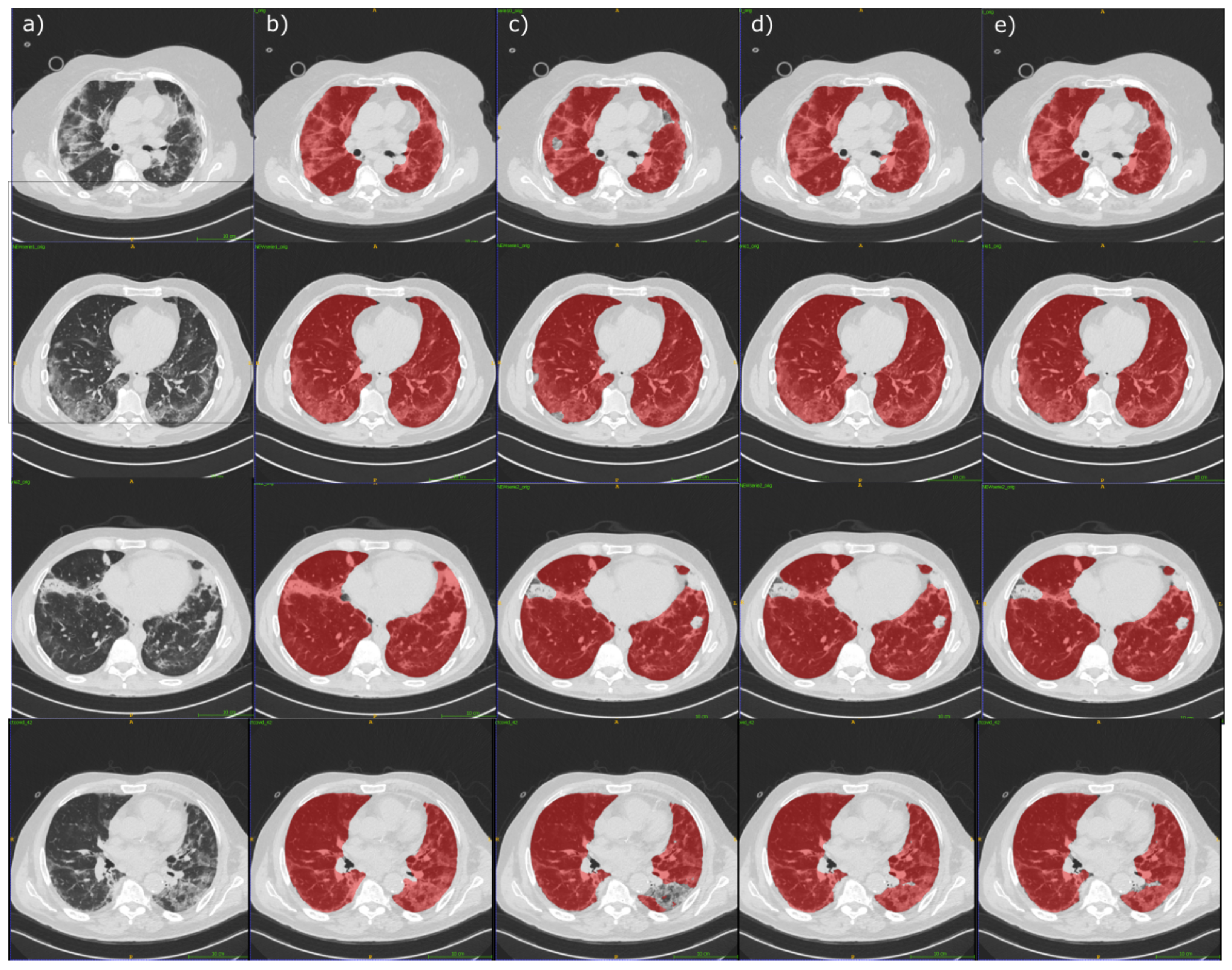
4.2. Segmentation Experimental Results

From the experiments conducted, we obtained the metrics reported in

Table 2. Experimental results for lung segmentation in COVID-19 patients from CT scans. LM stands for lung model, LLM stands for lung model plus lesion model. LLMPP stands for lung model plus lesion model plus post-processing.

Model	Precision [%]	Recall [%]	Dice [%]	RVD [%]	ASSD [mm]	MSSD [mm]
LM	$98.58\pm 0.92$	$95.58\pm 4.78$	$96.98\pm 2.46$	$-3.03\pm 5.16$	$1.68\pm 1.06$	$91.29\pm 33.67$
LLM	$98.35\pm 0.95$	$96.89\pm 3.42$	$97.58\pm 1.76$	$-1.47\pm 3.79$	$1.71\pm 0.92$	$96.21\pm 29.38$
LLMPP	$99.33\pm 0.49$	$95.77\pm 3.73$	$97.48\pm 1.98$	$-3.58\pm 3.86$	$0.95\pm 0.68$	$37.04\pm 27.03$

. Example CT scans, ground truth, and predictions can be seen from Figure 3.

It can be clearly observed that the lung model (LM) appears to have some troubles in predicting the whole lung region when it is highly lesioned. In order to overcome these difficulties, we combined it with a lesion model, resulting in the lung model plus lesion model (LLM) that is more likely to individuate the lung correctly with lesioned regions. Since the human body carries only two lungs, and they form a closed structure from a morphological point of view, applying post-processing based on morphological operators and connected component analysis can offer several benefits. In fact, it can be seen that MSSD is reduced from an average of more than 90 mm to an average of 37 mm with the lung model plus lesion model plus post-processing (LLMPP).

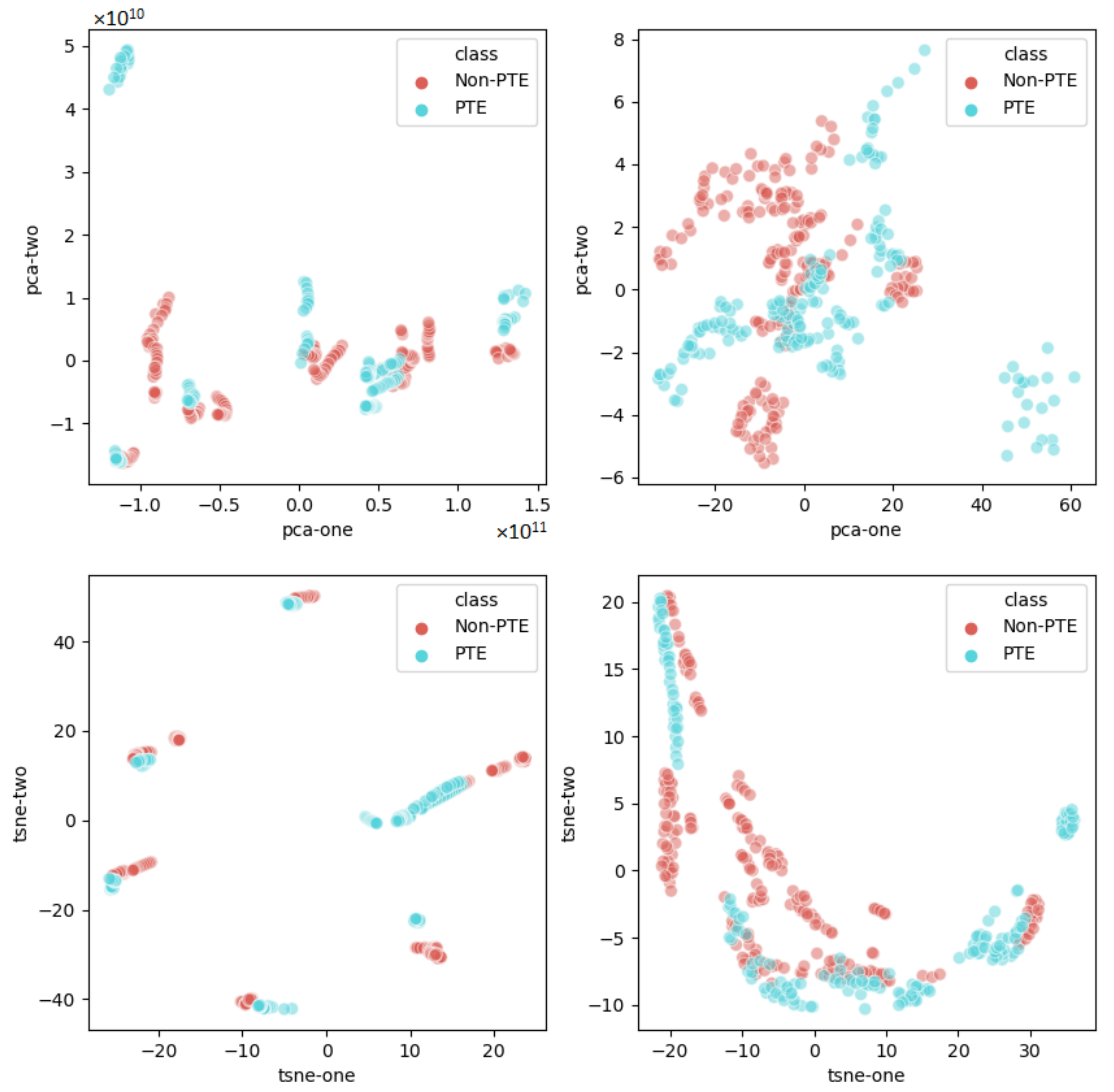
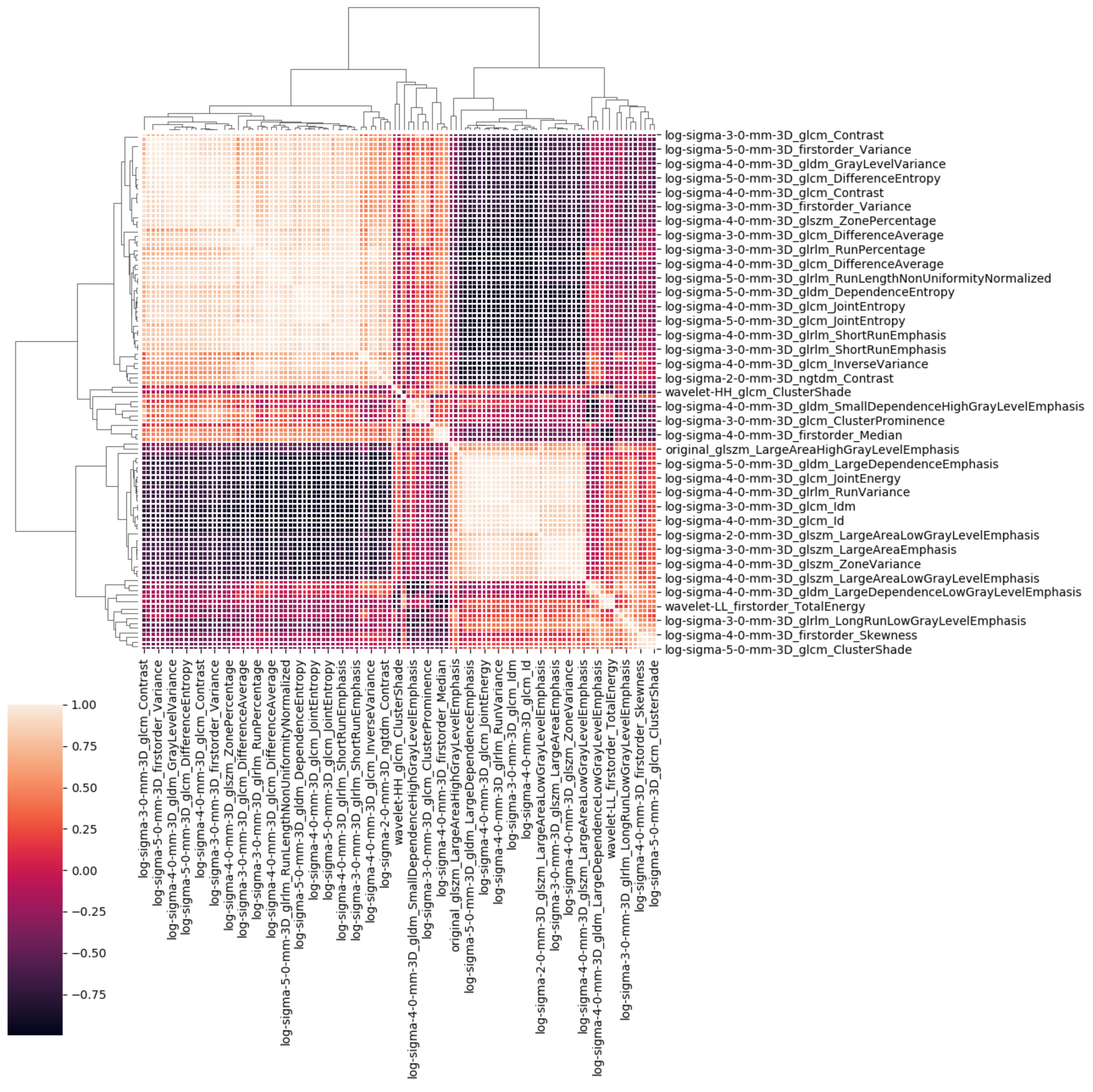
4.3. Radiomics Lung Characterization

In this phase, we investigated the features extracted from the 20 slices containing the largest portions of the lung from each CT scan in order to understand if there was a different feature distribution between patients who developed PTE or not. In order to obtain the mask of the lung, we exploited the methodology for semantic segmentation developed in Section 3.1 of this paper.

To the best of our knowledge, the possibility to characterize lung parenchyma and lesions with radiomics methodologies from COVID-19 patients, with respect to the onset of PTE, has never been explored before; therefore, this can be considered one of the main contributions of this paper.

We configured PyRadiomics, introduced in Section 3.2, to extract features by considering the original image, five versions of the image after having applied Laplacian of Gaussian (LoG), with sigma ranging from 1.0 to 5.0, and Wavelet versions of the image. Later, the subsequent classes of features were considered: 2D shape descriptors (shape2D), first-order statistics (firstorder), texture classes gray-level co-occurrence matrix (glcm) [52,53,54], gray-level run length matrix (glrlm) [55,56], gray-level size zone matrix (glszm) [57], gray-level dependence matrix (gldm) [58], neighboring gray tone difference matrix (ngtdm) [59].

CT scans were considered in a 2D slice-wise fashion on the axial plane, resampling x and y axes to a resolution of 1 mm, exploiting the sitkBSpline interpolator. According to PyRadiomics documentation, CT intensity values reflect absolute world values (HU), which should be comparable across scanners. In studies where multiple scanners are considered, researchers have to check if extracted features are correlated to the scanner adopted. However, given that we considered a cohort coming from the same hospital, problems of this kind do not occur. Image discretization was performed with a bin width set to 25, often considered as a default in PyRadiomics usage (e.g., https://pyradiomics.readthedocs.io/en/latest/customization.html, accessed on 8 October 2021). This process resulted in the extraction of 919 features for 400 samples (20 slices for each of the 20 CT scans).

We opted to visualize these features in a low-dimensionality space, by both considering principal component analysis (PCA) [60] and t-distributed stochastic neighbor embedding (t-SNE) [61]. For further visual understanding, the result of the 2D embedding space with PCA and t-SNE space is portrayed in Figure 4. No clear pattern emerged from either PCA or t-SNE embedding plots starting from the original feature space, but the feature representation improves after having selected a subset of uncorrelated and significant features.

Likewise, we performed a feature reduction procedure by considering statistical Mann–Whitney U tests on our radiomic feature set. In particular, we kept the features for which the corresponding corrected p-value was lesser than 0.01 (we tested their distribution for both PTE and non-PTE samples), resulting in an array of 109 features. The Holm–Šidák correction was exploited to counteract the multiple comparisons problem [62].

Starting from these 109 features, we investigated the correlation matrix with a cluster map (https://seaborn.pydata.org/generated/seaborn.clustermap.html, accessed on 8 October 2021), in order to assess the correlations between the features and eventually reduce the feature set. Cluster map performs hierarchical clustering. In our case, we used the unweighted pair group method with arithmetic mean (UPGMA) [63] clustering algorithm, with Euclidean distance as metric. To visualize the cluster map, kindly refer to Figure 5. A $5000\times 5000$ version of the same image is available in the supplementary materials, with all the feature names on both axes. It is possible to see that indeed there are clusters of correlated features. In particular, many features of the families glcm, glrlm, glszm show high correlation between the same family. Consequently, we proceeded to remove features with a correlation higher than 0.5, resulting in nine uncorrelated radiomic features that can be considered for the realization of a prognostic signature related to PTE assessment in COVID-19 patients. The procedure exploited for removing correlated features is reported in Algorithm 1.

The nine radiomic features we propose as prognostic signature are:

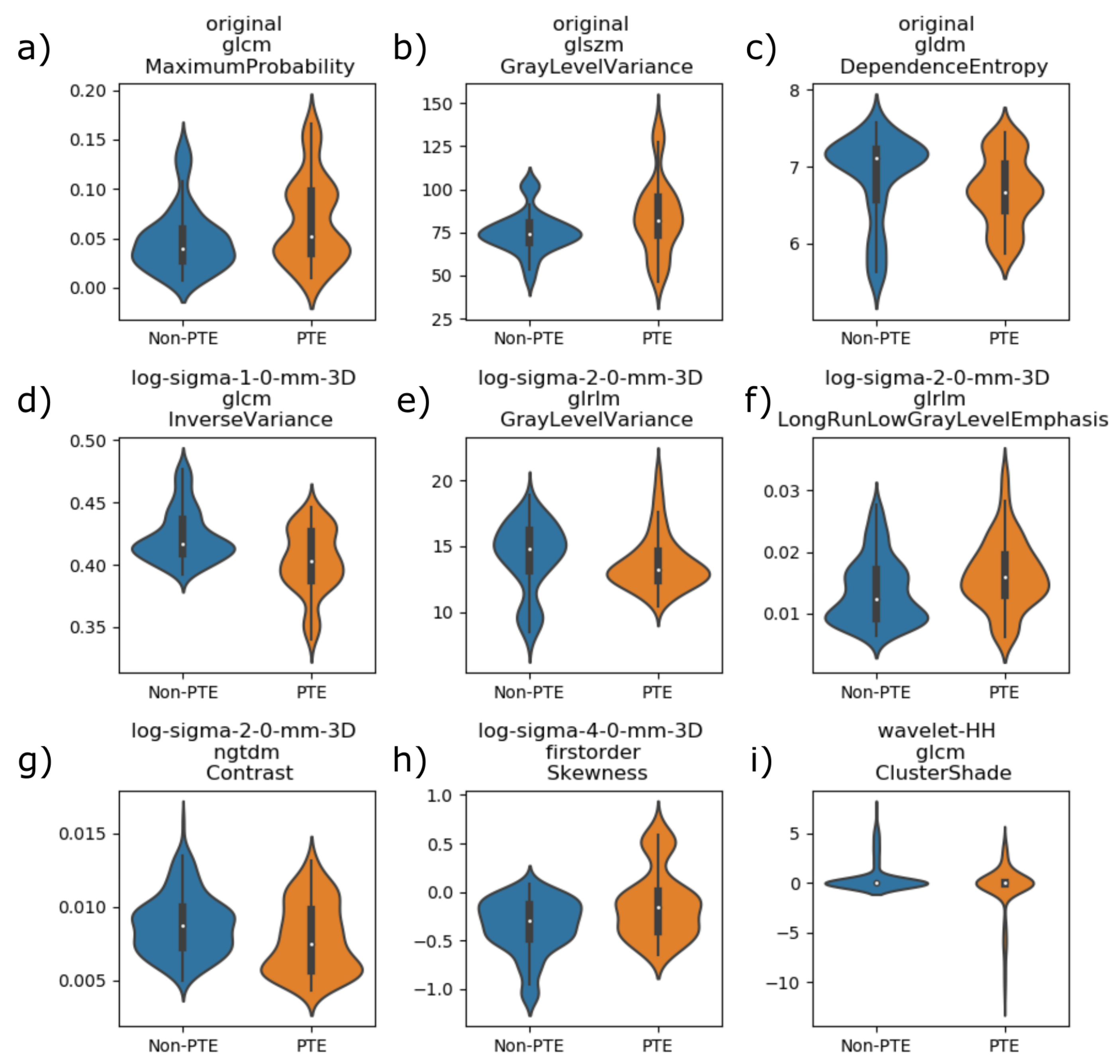
• original_glcm_MaximumProbability, defined in Equation (A2);
• original_glszm_GrayLevelVariance, defined in Equation (A11);
• original_gldm_DependenceEntropy, defined in Equation (A14);
• log-sigma-1-0-mm-3D_glcm_InverseVariance, defined in Equation (A4);
• log-sigma-2-0-mm-3D_glrlm_GrayLevelVariance, defined in Equation (A16);
• log-sigma-2-0-mm-3D_glrlm_LongRunLowGrayLevelEmphasis, defined in Equation (A18);
• log-sigma-2-0-mm-3D_ngtdm_Contrast, defined in Equation (A20);
• log-sigma-4-0-mm-3D_firstorder_Skewness, defined in Equation (A21);
• wavelet-HH_glcm_ClusterShade, defined in Equation (A5).

These feature names, derived from PyRadiomics, are composed of three parts, divided by the underscores.

Algorithm 1: Correlated Features Removal.

The first part refers to the image from which the features were extracted. It could be the original image (original), the image after having applied LoG with a given sigma (log-sigma-), or the image after having applied wavelet transform (wavelet-). In particular, four decompositions per level were obtained with Coiflets [64,65] from 2D slices; that is, all possible combinations of applying either a high or a low pass filter in each of the two dimensions. The parameter N of the Coiflets was set to 1 (e.g., see https://it.mathworks.com/help/wavelet/ref/coifwavf.html, last accessed: 8 October 2021).

The second part refers to the kind of features, as first-order statistical indicators (firstorder), second-order statistical indicators (as glcm or glrlm), and so on.

The last part refers to the specific feature name inside its family, as defined by the PyRadiomics documentation [44], which can be consulted for further information. Appendix A summarizes mathematical details and definitions for the features exploited in this study.

Violin plots showing the difference between distributions for PTE and non-PTE cases are reported in Figure 6. Statistics concerning the distributions of these features for PTE and non-PTE cases are reported in

Table 3. Statistics for feature distribution between PTE and non-PTE cases. Std is the standard deviation, IQR is the interquartile range. $U_{PTE}$ and $U_{Non-PTE}$ are the two-sided U statistics.

Feature	Mean		Median		Std		IQR		${\mathit{U}}_{\mathbf{PTE}}$	${\mathit{U}}_{\mathbf{Non}-\mathbf{PTE}}$
	Non-PTE	PTE	Non-PTE	PTE	Non-PTE	PTE	Non-PTE	PTE
1	0.0485	0.0683	0.0390	0.0519	0.0322	0.0430	0.0325	0.0644	24,999	14,601
2	749.736	843.911	742.459	821.026	119.081	218.129	110.752	218.576	25,849	13,751
3	68.824	66.891	71.056	66.667	0.5538	0.4505	0.6482	0.5939	14,637	24,963
4	0.4233	0.4029	0.4162	0.4032	0.0210	0.0258	0.0269	0.0389	11,459	28,141
5	142.651	137.572	148.364	132.101	26.378	20.881	30.981	22.403	14,731	24,869
6	0.0137	0.0164	0.0123	0.0160	0.0053	0.0057	0.0079	0.0065	25,470	14,130
7	0.0088	0.0078	0.0087	0.0074	0.0021	0.0024	0.0027	0.0041	14,680	24,920
8	−0.3484	−0.1261	−0.2963	−0.1591	0.2789	0.3489	0.3635	0.4178	25,838	13,762
9	0.6364	−0.4777	−0.0010	−0.0092	15.061	24.794	0.0544	0.0322	14,646	24,954

.

5. Discussion

Several authors have already dealt with the problem of COVID-19 detection from CT scans [12,17,18,21,22] or focused on the task of lung and lesion segmentation [13,15,16,17,20,21,22]. In our cohort, all of the patients were positive to COVID-19, since the objective was not that of realizing another algorithm for COVID-19 diagnosis. The methods, materials, and results adopted by the related works are summarized in

Table 4. Literature overview for various COVID-19 image tasks, as segmentation, detection, and classification. CT stands for computed tomography, ROC stands for receiver operating characteristic, IoU stands for intersection over union, AUC stands for area under the curve, AP stands for average precision, NPV stands for negative predictive value, PR stands for precision-recall, MCC stands for Matthews correlation coefficient, CNN stands for convolutional neural network, FCN stands for fully convolutional network, R-CNN stands for region-based convolutional neural network, DPN stands for dual path network, FRAGL stands for fuzzy region-based active contours driven by weighting global and local fitting energy.

Author	Method	Materials	Task	Results
Wu et al. [12]	Joint classification and segmentation (JCS)	144,167 CT images (3855 annotated)	Real-time and explainable COVID-19 classification	Classification: sensitivity = 0.95, specificity = 0.93; segmentation: Dice = 0.78
Akbari et al. [13]	Active Contour	100 CT images	COVID-19 lesions segmentation	FRAGL: Dice = 0.96, Jaccard = 0.93, F1 = 0.66, precision = 0.91, recall = 0.53
Cao et al. [14]	U-Net-like CNN	2 CT scans	Objective assessment of pulmonary involvement and therapy response in COVID-19	Qualitative
Rajinikanth et al. [15]	Firefly algorithm and multi-thresholding based on Shannon entropy + Markov Random Field segmentation	100 CT images	COVID-19 lesions segmentation	Jaccard = 0.84, Dice = 0.89, accuracy = 0.92, precision = 0.92, sensitivity = 0.95, specificity = 0.94, NPV = 0.93
Rajinikanth et al. [16]	Harmony search optimization and Otsu thresholding	90 CT coronal slices + 20 CT axial slices	COVID-19 lesion segmentation	Infection rate
Ter-Sarkisov et al. [17]	One shot model based on Mask R-CNN	750 CT images for segmentation + 1492 for classification	COVID-19 classification and lesions segmentation	Segmentation: [email protected] IoU = 0.614, Classification: accuracy = 0.91
Zhao et al. [18]	Multi-task learning and self-supervised learning	349 COVID-19 CT images + 463 non-COVID-19 CT images	COVID-19 classification	F1 = 0.90, AUC = 0.98, accuracy = 0.89
Wang et al. [19]	Segmentation: FCN, U-Net, V-Net, 3D U-Net++; Classification: ResNet-50, inception, DPN-92, attention ResNet-50	1136 CT images	COVID-19 pneumonia detection	Sensitivity = 0.97, specificity = 0.92, AUC = 0.991
Oulefki et al. [20]	Improved Kapur entropy-based multilevel thresholding procedure	275 CT images from COVID-CT-dataset + 22 CT images (local)	COVID-19 lesions segmentation	Accuracy = 0.98, sensitivity = 0.73, F1 = 0.71, precision = 0.73, MCC = 0.71, Dice = 0.71, Jaccard = 0.57, specificity = 0.99
Zheng, Wang et al. [21,22]	U-Net + 3D deep neural network	499 CT volumes (train) + 131 CT volumes (test)	Lung segmentation + COVID-19 classification	ROC AUC = 0.96, PR AUC = 0.98, sensitivity = 0.91, specificity = 0.91

. It is possible to see that COVID-19 classification algorithms manage to obtain high performances. In regard to the segmentation, it is worth noting that some authors did not provide quantitative comparable metrics [14,16]. Other authors provided metrics for lesions segmentation, but not for lung parenchyma and lesion joint segmentation. Nonetheless, it is possible to see from our experiments that our model is better at segmenting lungs with respect to models that have been trained only on non-COVID-19 patients. To the best of our knowledge, no other work in the literature considered the possibility of exploiting radiomics methodologies in order to characterize the lungs between PTE and non-PTE patients. As can be seen from Figure 6 and Table 3, the designated features show different characteristics, from a statistical point of view, among the two conditions. This can aid in posing the basis for the development of a reliable predictive model, which will need to be tested on external and larger validation sets. Instead, in this work, we focused on the feature selection and statistical analysis stage.

6. Conclusions and Future Works

The COVID-19 pandemic has led to drastic impacts in our world. To address the deadliest complications from COVID-19, CT scans are routinely adopted in diagnostic and prognostic procedures. The task of manually segmenting lung parenchyma and lesions is tedious and error-prone, and it can suffer from intra- and inter-operator variability. Therefore, we proposed an automated workflow for segmenting lung lesions and parenchyma, aiding the work of radiologists and posing the basis for further analysis on the segmented region. The segmentation allowed to obtain accurate results with a mean Dice coefficient of 97.48% and a mean ASSD of 0.95 mm for the chosen model. We also addressed the problem of finding a prognostic signature that can be used to characterize the risk of onset of PTE, deriving nine uncorrelated features that show significantly different statistical distributions according to the Mann–Whitney U test. However, more data need to be acquired in order to better understand the generalizability of the discovered feature set, which is considered as part of future work.

References

1. Grillet, F.; Behr, J.; Calame, P.; Aubry, S.; Delabrousse, E. Acute Pulmonary Embolism Associated with COVID-19 Pneumonia Detected with Pulmonary CT Angiography. Radiology 2020, 296, E186–E188. [Google Scholar] [CrossRef] [PubMed] [Green Version]
2. Léonard-Lorant, I.; Delabranche, X.; Séverac, F.; Helms, J.; Pauzet, C.; Collange, O.; Schneider, F.; Labani, A.; Bilbault, P.; Molière, S.; et al. Acute Pulmonary Embolism in Patients with COVID-19 at CT Angiography and Relationship to d-Dimer Levels. Radiology 2020, 296, E189–E191. [Google Scholar] [CrossRef] [PubMed] [Green Version]
3. Scardapane, A.; Villani, L.; Bavaro, D.F.; Passerini, F.; Ianora, A.A.S.; Lucarelli, N.M.; Angarano, G.; Portincasa, P.; Palmieri, V.O.; Saracino, A. Pulmonary Artery Filling Defects in COVID-19 Patients Revealed Using CT Pulmonary Angiography: A Predictable Complication? BioMed Res. Int. 2021, 2021. [Google Scholar] [CrossRef] [PubMed]
4. Bavaro, D.F.; Poliseno, M.; Scardapane, A.; Belati, A.; De Gennaro, N.; Stabile Ianora, A.A.; Angarano, G.; Saracino, A. Occurrence of Acute Pulmonary Embolism in COVID-19-A case series. Int. J. Infect. Dis. IJID Off. Publ. Int. Soc. Infect. Dis. 2020, 98, 225–226. [Google Scholar] [CrossRef]
5. Mukherjee, H.; Ghosh, S.; Dhar, A.; Obaidullah, S.M.; Santosh, K.C.; Roy, K. Shallow Convolutional Neural Network for COVID-19 Outbreak Screening using Chest X-rays. Cogn Comput 2021. [Google Scholar] [CrossRef]
6. Cobelli, R.; Zompatori, M.; De Luca, G.; Chiari, G.; Bresciani, P.; Marcato, C. Clinical usefulness of computed tomography study without contrast injection in the evaluation of acute pulmonary embolism. J. Comput. Assist. Tomogr. 2005, 29, 6–12. [Google Scholar] [CrossRef]
7. Remy-Jardin, M.; Faivre, J.B.; Kaergel, R.; Hutt, A.; Felloni, P.; Khung, S.; Lejeune, A.L.; Giordano, J.; Remy, J. Machine Learning and Deep Neural Network Applications in the Thorax: Pulmonary Embolism, Chronic Thromboembolic Pulmonary Hypertension, Aorta, and Chronic Obstructive Pulmonary Disease. J. Thorac. Imaging 2020, 35, S40–S48. [Google Scholar] [CrossRef]
8. Yousef, H.A.Z. The accuracy of non-contrast chest computed tomographic Scan in the detection of pulmonary thromboembolism. J. Curr. Med. Res. Pract. 2019, 61–66. [Google Scholar] [CrossRef]
9. Sun, S.; Semionov, A.; Xie, X.; Kosiuk, J.; Mesurolle, B. Detection of central pulmonary embolism on non-contrast computed tomography: A case control study. Int. J. Cardiovasc. Imaging 2014, 30, 639–646. [Google Scholar] [CrossRef]
10. Tourassi, G.D.; Floyd, C.E.; Sostman, H.D.; Coleman, R.E. Acute pulmonary embolism: Artificial neural network approach for diagnosis. Radiology 1993, 189, 555–558. [Google Scholar] [CrossRef]
11. Jimenez-del Toro, O.; Dicente Cid, Y.; Platon, A.; Hachulla, A.L.; Lador, F.; Poletti, P.A.; Müller, H. A lung graph model for the radiological assessment of chronic thromboembolic pulmonary hypertension in CT. Comput. Biol. Med. 2020, 125, 103962. [Google Scholar] [CrossRef] [PubMed]
12. Wu, Y.H.; Gao, S.H.; Mei, J.; Xu, J.; Fan, D.P.; Zhao, C.W.; Cheng, M.M. JCS: An explainable COVID-19 diagnosis system by joint classification and segmentation. arXiv 2020, arXiv:2004.07054. [Google Scholar]
13. Akbari, Y.; Hassen, H.; Al-maadeed, S.; Zughaier, S. COVID-19 Lesion Segmentation using Lung CT Scan Images: Comparative Study based on Active Contour Models. Appl. Sci. 2021, 11, 8039. [Google Scholar] [CrossRef]
14. Cao, Y.; Xu, Z.; Feng, J.; Jin, C.; Han, X.; Wu, H.; Shi, H. Longitudinal Assessment of COVID-19 Using a Deep Learning–based Quantitative CT Pipeline: Illustration of Two Cases. Radiol. Cardiothorac. Imaging 2020, 2, e200082. [Google Scholar] [CrossRef] [Green Version]
15. Rajinikanth, V.; Kadry, S.; Thanaraj, K.P.; Kamalanand, K.; Seo, S. Firefly-algorithm supported scheme to detect COVID-19 lesion in lung CT scan images using shannon entropy and markov-random-field. arXiv 2020, arXiv:2004.09239. [Google Scholar]
16. Rajinikanth, V.; Dey, N.; Raj, A.N.J.; Hassanien, A.E.; Santosh, K.C.; Raja, N.S.M. Harmony-Search and Otsu based System for Coronavirus Disease (COVID-19) Detection using Lung CT Scan Images. arXiv 2020, arXiv:2004.03431. [Google Scholar]
17. Ter-Sarkisov, A. One Shot Model For The Prediction of COVID-19 and Lesions Segmentation In Chest CT Scans Through The Affinity Among Lesion Mask Features. medRxiv 2021. [Google Scholar] [CrossRef]
18. Zhao, J.; He, X.; Yang, X.; Zhang, Y.; Zhang, S.; Xie, P. COVID-CT-Dataset: A CT image dataset about COVID-19. arXiv 2020, arXiv:2003.13865. [Google Scholar]
19. Wang, B.; Jin, S.; Yan, Q.; Xu, H.; Luo, C.; Wei, L.; Zhao, W.; Hou, X.; Ma, W.; Xu, Z.; et al. AI-assisted CT imaging analysis for COVID-19 screening: Building and deploying a medical AI system. Appl. Soft Comput. 2021, 98, 106897. [Google Scholar] [CrossRef]
20. Oulefki, A.; Agaian, S.; Trongtirakul, T.; Kassah Laouar, A. Automatic COVID-19 lung infected region segmentation and measurement using CT-scans images. Pattern Recognit. 2020, 107747. [Google Scholar] [CrossRef]
21. Zheng, C.; Deng, X.; Fu, Q.; Zhou, Q.; Feng, J.; Ma, H.; Liu, W.; Wang, X. Deep Learning-based Detection for COVID-19 from Chest CT using Weak Label. medRxiv 2020, 1–13. [Google Scholar] [CrossRef] [Green Version]
22. Wang, X.; Deng, X.; Fu, Q.; Zhou, Q.; Feng, J.; Ma, H.; Liu, W.; Zheng, C. A Weakly-Supervised Framework for COVID-19 Classification and Lesion Localization from Chest CT. IEEE Trans. Med. Imaging 2020, 39, 2615–2625. [Google Scholar] [CrossRef]
23. He, K.; Gkioxari, G.; Dollár, P.; Girshick, R.; Dollar, P.; Girshick, R. Mask R-CNN. In Proceedings of the IEEE International Conference on Computer Vision, Venice, Italy, 22–29 October 2017; pp. 2980–2988. [Google Scholar] [CrossRef]
24. Ma, J.; Ge, C.; Wang, Y.; An, X.; Gao, J.; Yu, Z.; Zhang, M.; Liu, X.; Deng, X.; Cao, S.; et al. COVID-19 CT Lung and Infection Segmentation Dataset. Zenodo 2020. [Google Scholar] [CrossRef]
25. Zaffino, P.; Marzullo, A.; Moccia, S.; Calimeri, F.; De Momi, E.; Bertucci, B.; Arcuri, P.P.; Spadea, M.F. An open-source covid-19 ct dataset with automatic lung tissue classification for radiomics. Bioengineering 2021, 8, 26. [Google Scholar] [CrossRef]
26. LeCun, Y.; Bengio, Y.; Hinton, G. Deep learning. Nature 2015, 521, 436–444. [Google Scholar] [CrossRef]
27. Altini, N.; Cascarano, G.D.; Brunetti, A.; De Feudis, D.I.; Buongiorno, D.; Rossini, M.; Pesce, F.; Gesualdo, L.; Bevilacqua, V. A Deep Learning Instance Segmentation Approach for Global Glomerulosclerosis Assessment in Donor Kidney Biopsies. Electronics 2020, 9, 1768. [Google Scholar] [CrossRef]
28. Brunetti, A.; Carnimeo, L.; Trotta, G.F.; Bevilacqua, V. Computer-assisted frameworks for classification of liver, breast and blood neoplasias via neural networks: A survey based on medical images. Neurocomputing 2019, 335, 274–298. [Google Scholar] [CrossRef]
29. Lateef, F.; Ruichek, Y. Survey on semantic segmentation using deep learning techniques. Neurocomputing 2019, 338, 321–348. [Google Scholar] [CrossRef]
30. Altini, N.; Cascarano, G.D.; Brunetti, A.; Marino, F.; Rocchetti, M.T.; Matino, S.; Venere, U.; Rossini, M.; Pesce, F.; Gesualdo, L.; et al. Semantic Segmentation Framework for Glomeruli Detection and Classification in Kidney Histological Sections. Electronics 2020, 9, 503. [Google Scholar] [CrossRef] [Green Version]
31. Bevilacqua, V.; Brunetti, A.; Cascarano, G.D.; Guerriero, A.; Pesce, F.; Moschetta, M.; Gesualdo, L. A comparison between two semantic deep learning frameworks for the autosomal dominant polycystic kidney disease segmentation based on magnetic resonance images. BMC Med. Inform. Decis. Mak. 2019, 19, 244. [Google Scholar] [CrossRef]
32. Liu, L.; Cheng, J.; Quan, Q.; Wu, F.X.; Wang, Y.P.; Wang, J. A survey on U-shaped networks in medical image segmentations. Neurocomputing 2020, 409, 244–258. [Google Scholar] [CrossRef]
33. Ronneberger, O.; Fischer, P.; Brox, T. U-net: Convolutional networks for biomedical image segmentation. Lect. Notes Comput. Sci. (Incl. Subser. Lect. Notes Artif. Intell. Lect. Notes Bioinform.) 2015, 9351, 234–241. [Google Scholar] [CrossRef] [Green Version]
34. Cicek, O.; Abdulkadir, A.; Lienkamp, S.S.; Brox, T.; Ronneberger, O. 3D U-Net: Learning Dense Volumetric Segmentation from Sparse Annotation. Lect. Notes Comput. Sci. (Incl. Subser. Lect. Notes Artif. Intell. Lect. Notes Bioinform.) 2016, 9901, 424–432. [Google Scholar] [CrossRef] [Green Version]
35. Milletari, F.; Navab, N.; Ahmadi, S.A.A. V-Net: Fully Convolutional Neural Networks for Volumetric Medical Image Segmentation. In Proceedings of the 2016 fourth international conference on 3D vision (3DV), Stanford, CA, USA, 25–28 October 2016; pp. 565–571. [Google Scholar] [CrossRef] [Green Version]
36. Altini, N.; Prencipe, B.; Brunetti, A.; Brunetti, G.; Triggiani, V.; Carnimeo, L.; Marino, F.; Guerriero, A.; Villani, L.; Scardapane, A.; et al. A Tversky Loss-Based Convolutional Neural Network for Liver Vessels Segmentation; Springer: Cham, Switzerland, 2020; Volume 12463. [Google Scholar] [CrossRef]
37. Altini, N.; De Giosa, G.; Fragasso, N.; Coscia, C.; Sibilano, E.; Prencipe, B.; Hussain, S.M.; Brunetti, A.; Buongiorno, D.; Guerriero, A.; et al. Segmentation and Identification of Vertebrae in CT Scans Using CNN, k-Means Clustering and k-NN. Informatics 2021, 8, 40. [Google Scholar] [CrossRef]
38. Lambin, P.; Rios-Velazquez, E.; Leijenaar, R.; Carvalho, S.; Van Stiphout, R.G.; Granton, P.; Zegers, C.M.; Gillies, R.; Boellard, R.; Dekker, A.; et al. Radiomics: Extracting more information from medical images using advanced feature analysis. Eur. J. Cancer 2012, 48, 441–446. [Google Scholar] [CrossRef] [Green Version]
39. Le, N.Q.K.; Kha, Q.H.; Nguyen, V.H.; Chen, Y.C.; Cheng, S.J.; Chen, C.Y. Machine Learning-Based Radiomics Signatures for EGFR and KRAS Mutations Prediction in Non-Small-Cell Lung Cancer. Int. J. Mol. Sci. 2021, 22, 9254. [Google Scholar] [CrossRef]
40. Aerts, H.J.; Velazquez, E.R.; Leijenaar, R.T.; Parmar, C.; Grossmann, P.; Cavalho, S.; Bussink, J.; Monshouwer, R.; Haibe-Kains, B.; Rietveld, D.; et al. Decoding tumour phenotype by noninvasive imaging using a quantitative radiomics approach. Nat. Commun. 2014, 5. [Google Scholar] [CrossRef]
41. Le, N.Q.K.; Hung, T.N.K.; Do, D.T.; Lam, L.H.T.; Dang, L.H.; Huynh, T.T. Radiomics-based machine learning model for efficiently classifying transcriptome subtypes in glioblastoma patients from MRI. Comput. Biol. Med. 2021, 132, 104320. [Google Scholar] [CrossRef]
42. Bevilacqua, V.; Brunetti, A.; Trotta, G.F.; Dimauro, G.; Elez, K.; Alberotanza, V.; Scardapane, A. A novel approach for Hepatocellular Carcinoma detection and classification based on triphasic CT Protocol. In Proceedings of the 2017 IEEE Congress on Evolutionary Computation (CEC), Donostia, Spain, 5–8 June 2017; pp. 1856–1863. [Google Scholar]
43. Pinker, K.; Chin, J.; Melsaether, A.N.; Morris, E.A.; Moy, L. Precision medicine and radiogenomics in breast cancer: New approaches toward diagnosis and treatment. Radiology 2018, 287, 732–747. [Google Scholar] [CrossRef]
44. Van Griethuysen, J.J.; Fedorov, A.; Parmar, C.; Hosny, A.; Aucoin, N.; Narayan, V.; Beets-Tan, R.G.; Fillion-Robin, J.C.; Pieper, S.; Aerts, H.J. Computational radiomics system to decode the radiographic phenotype. Cancer Res. 2017, 77, e104–e107. [Google Scholar] [CrossRef] [Green Version]
45. Zwanenburg, A.; Leger, S.; Vallières, M.; Löck, S. Image biomarker standardisation initiative. arXiv 2016, arXiv:1612.07003. [Google Scholar]
46. Gillies, R.J.; Kinahan, P.E.; Hricak, H. Radiomics: Images are more than pictures, they are data. Radiology 2016, 278, 563–577. [Google Scholar] [CrossRef] [PubMed] [Green Version]
47. Kumar, V.; Gu, Y.; Basu, S.; Berglund, A.; Eschrich, S.A.; Schabath, M.B.; Forster, K.; Aerts, H.J.; Dekker, A.; Fenstermacher, D.; et al. Radiomics: The process and the challenges. Magn. Reson. Imaging 2012, 30, 1234–1248. [Google Scholar] [CrossRef] [PubMed] [Green Version]
48. Rizzo, S.; Botta, F.; Raimondi, S.; Origgi, D.; Fanciullo, C.; Morganti, A.G.; Bellomi, M. Radiomics: The facts and the challenges of image analysis. Eur. Radiol. Exp. 2018, 2. [Google Scholar] [CrossRef]
49. Heimann, T.; van Ginneken, B.; Styner, M.M.A.; Arzhaeva, Y.; Aurich, V.; Bauer, C.; Beck, A.; Becker, C.; Beichel, R.; Bekes, G.; et al. Comparison and Evaluation of Methods for Liver Segmentation From CT Datasets. IEEE Trans. Med. Imaging 2009, 28, 1251–1265. [Google Scholar] [CrossRef]
50. Bilic, P.; Christ, P.F.; Vorontsov, E.; Chlebus, G.; Chen, H.; Dou, Q.; Fu, C.W.; Han, X.; Heng, P.A.; Hesser, J.; et al. The Liver Tumor Segmentation Benchmark (LiTS). arXiv 2019, arXiv:1901.04056. [Google Scholar]
51. Prencipe, B.; Altini, N.; Cascarano, G.D.; Guerriero, A.; Brunetti, A. A Novel Approach Based on Region Growing Algorithm for Liver and Spleen Segmentation from CT Scans. In Intelligent Computing Theories and Application; Huang, D.S., Bevilacqua, V., Hussain, A., Eds.; Springer International Publishing: Cham, Switzerland, 2020; pp. 398–410. [Google Scholar]
52. Haralick, R.M.; Dinstein, I.; Shanmugam, K. Textural Features for Image Classification. IEEE Trans. Syst. Man Cybern. 1973, SMC-3, 610–621. [Google Scholar] [CrossRef] [Green Version]
53. Bevilacqua, V.; Pietroleonardo, N.; Triggiani, V.; Brunetti, A.; Di Palma, A.M.; Rossini, M.; Gesualdo, L. An innovative neural network framework to classify blood vessels and tubules based on Haralick features evaluated in histological images of kidney biopsy. Neurocomputing 2017, 228, 143–153. [Google Scholar] [CrossRef]
54. Altini, N.; Marvulli, T.M.; Caputo, M.; Mattioli, E.; Prencipe, B.; Cascarano, G.D.; Brunetti, A.; Tommasi, S.; Bevilacqua, V.; De Summa, S.; et al. Multi-class Tissue Classification in Colorectal Cancer with Handcrafted and Deep Features. In Intelligent Computing Theories and Application; Huang, D.S., Jo, K.H., Li, J., Gribova, V., Bevilacqua, V., Eds.; Springer International Publishing: Cham, Switzerland, 2021; pp. 512–525. [Google Scholar]
55. Galloway, M.M. Texture analysis using gray level run lengths. Comput. Graph. Image Process. 1975, 4, 172–179. [Google Scholar] [CrossRef]
56. Chu, A.; Sehgal, C.M.; Greenleaf, J.F. Use of gray value distribution of run lengths for texture analysis. Pattern Recognit. Lett. 1990, 11, 415–419. [Google Scholar] [CrossRef]
57. Thibault, G.; Fertil, B.; Navarro, C.; Pereira, S.; Cau, P.; Levy, N.; Sequeira, J.; Mari, J.-L. Texture Indexes and Gray Level Size Zone Matrix Application to Cell Nuclei Classification. In Proceedings of the 10th International Conference on Pattern Recognition and Information Processing, Minsk, Belarus, 19–21 May 2009; pp. 140–145. [Google Scholar]
58. Sun, C.; Wee, W.G. Neighboring gray level dependence matrix for texture classification. Comput. Vis. Graph. Image Process. 1983, 23, 341–352. [Google Scholar] [CrossRef]
59. Amadasun, M.; King, R. Textural features corresponding to textural properties. IEEE Trans. Syst. Man Cybern. 1989, 19, 1264–1274. [Google Scholar] [CrossRef]
60. Song, F.; Guo, Z.; Mei, D. Feature Selection Using Principal Component Analysis. In Proceedings of the 2010 International Conference on System Science, Engineering Design and Manufacturing Informatization, Yichang, China, 12–14 November 2010; Volume 1, pp. 27–30. [Google Scholar] [CrossRef]
61. der Maaten, L.; Hinton, G. Visualizing data using t-SNE. J. Mach. Learn. Res. 2008, 9, 2579–2605. [Google Scholar]
62. Šidák, Z. Rectangular Confidence Regions for the Means of Multivariate Normal Distributions. J. Am. Stat. Assoc. 1967, 62, 626–633. [Google Scholar] [CrossRef]
63. Weiß, M.; Göker, M. Chapter 12 - Molecular Phylogenetic Reconstruction. In The Yeasts (Fifth Edition), 5th ed.; Kurtzman, C.P., Fell, J.W., Boekhout, T., Eds.; Elsevier: London, UK, 2011; pp. 159–174. [Google Scholar] [CrossRef]
64. Beylkin, G.; Coifman, R.; Rokhlin, V. Fast wavelet transforms and numerical algorithms. In Fundamental Papers in Wavelet Theory; Princeton University Press: Princeton, NJ, USA, 2009; pp. 741–783. [Google Scholar]
65. Daubechies, I. Ten Lectures on Wavelets; SIAM: Philadelphia, PA, USA, 1992. [Google Scholar]
Figure 1. Top row: CT scans from our local dataset from the Polyclinic of Bari. Bottom row: annotations provided by expert radiologists. Green denotes ground-glass opacity (GGO), whereas blue indicates lung consolidation (LC).
Electronics 10 02475 g001
Figure 2. Workflow for segmentation of lung parenchyma and lesion. CT scans, coming from three datasets, are clipped to [ 1250 , 250 ] and then normalized by rescaling in the range [ 0 , 1 ] . Two separate models are trained, a 2.5D V-Net exploiting T1 and T2, and a 2D V-Net exploiting T3. Final results are obtained by merging the masks from the two models with the logical OR operation. Metrics are assessed on the union of V1, V2, and V3 validation sets.
Electronics 10 02475 g002
Figure 3. Example CT scans and predictions: (a) original CT scans; (b) ground truth from radiologists at the Polyclinic of Bari; (c) lung model predictions; (d) lung model predictions combined with lesions predictions; (e) lung model predictions combined with lesions predictions, after post-processing.
Electronics 10 02475 g003
Figure 4. Visualizing radiomic features in the 2D PCA and t-SNE spaces. (Top left) PCA starting from the 919 features; (top right) PCA starting from the radiomics signature of nine uncorrelated and significant features; (bottom left) t-SNE starting from the 919 features; (bottom right) t-SNE starting from the radiomics signature of nine uncorrelated and significant features.
Electronics 10 02475 g004
Figure 5. Cluster map for the 109 features, which have corrected p-value lesser than 0.01.
Electronics 10 02475 g005
Figure 6. Violin plots for the subset of 9 significant and uncorrelated features, that have been selected exploiting Algorithm 1: (a) glcm maximum probability of the original image; (b) glcm gray level variance of the original image; (c) gldm dependence entropy of the original image; (d) glcm inverse variance of the LoG (Laplacian of a Gaussian) version of the image with σ = 1 ; (e) glrlm gray level variance of the LoG version of the image with σ = 2 ; (f) glrlm long run low gray level emphasis of the LoG version of the image with σ = 2 ; (g) ngtdm contrast of the LoG version of the image with σ = 2 ; (h) histogram skewness of the LoG version of the image with σ = 4 ; (i) glcm cluster shade of the HH wavelet version of the image. Scales of values on y axis have to be multiplied by a factor of 10 for the plots: (b,c,e).
Electronics 10 02475 g006