
Verification in Relevant Environment of a Physics-Based Synthetic Sensor for Flow Angle Estimation †


Abstract
:1. Introduction
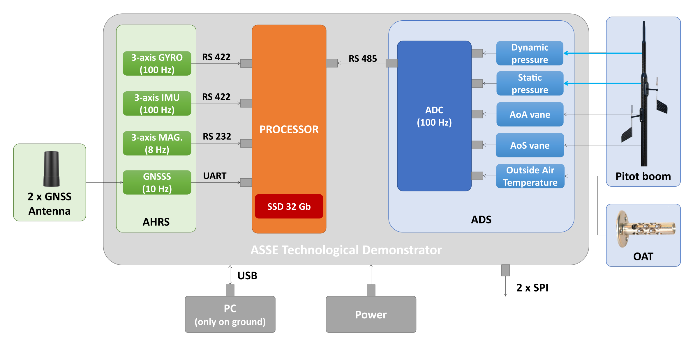
2. The ASSE Technological Demonstrator Concept
- from the Air data System (ADS):
- 1.
- Dynamic pressure (or, as alternative, total pressure);
- 2.
- Absolute pressure ;
- 3.
- Ambient temperature T;
- 4.
- Angle-of-attack AoA (as a reference value);
- 5.
- Angle-of-sideslip AoS (as a reference value);
- from the Attitude and Heading Reference System (AHRS):
- 6.
- 3-axis angular rates;
- 7.
- 3-axis linear accelerations;
- 8.
- 3-axis magnetometer;
- 9.
- 2-axis inclinometer;
- 10.
- GNSS position and velocity;
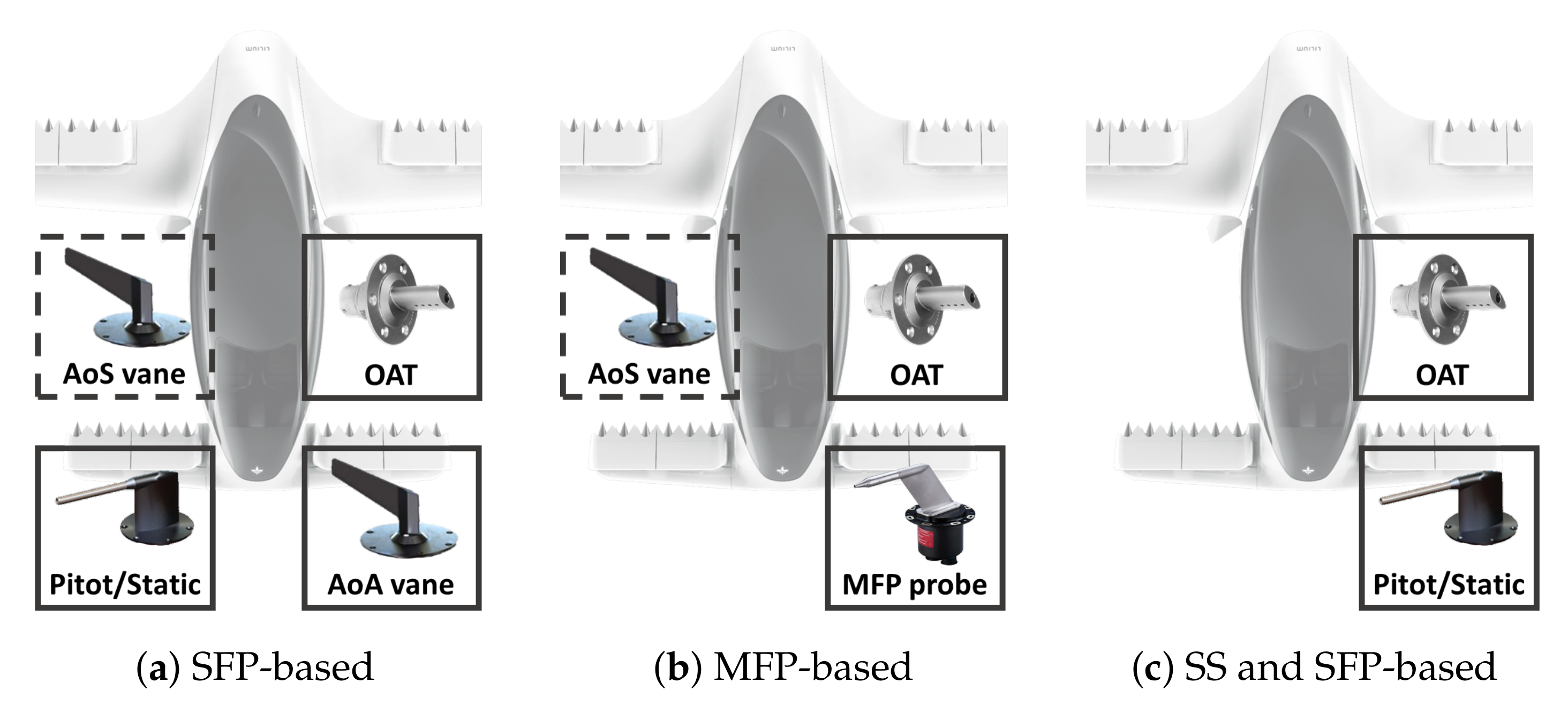
2.1. State-of-the-Art of Air Data System Sensors
2.2. Demonstrator’s Architecture
2.3. Attitude, Heading and Reference Sub-System
2.4. Air Data Sub-System
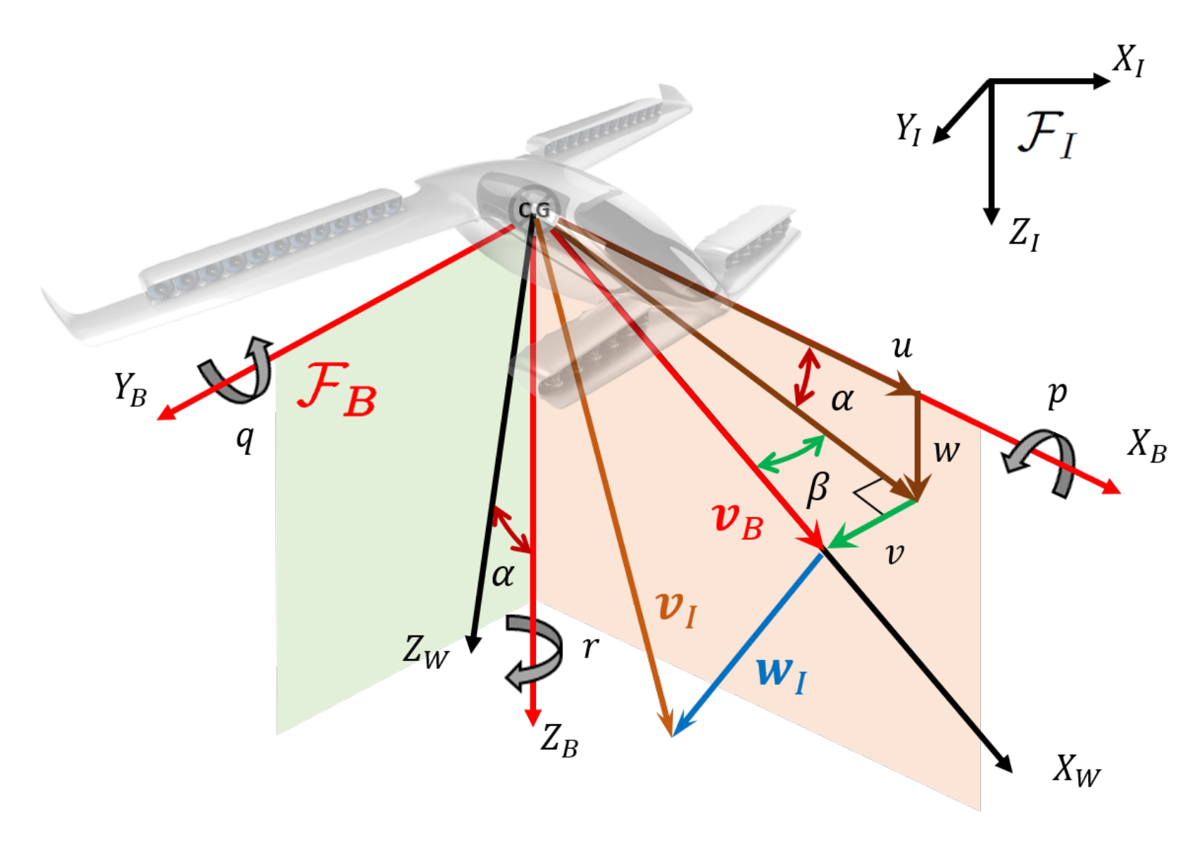
3. Nonlinear ASSE Scheme
3.1. The ASSE Synopsis
3.2. Practical Implementation
- vertical/lateral inertial acceleration:
- for AoA estimation
- for AoS estimation
- determinant of Equation (18): ,
- maximum absolute error <5°
- error <2°.
4. Characterisation of the ASSE Demonstrator’s Sensors
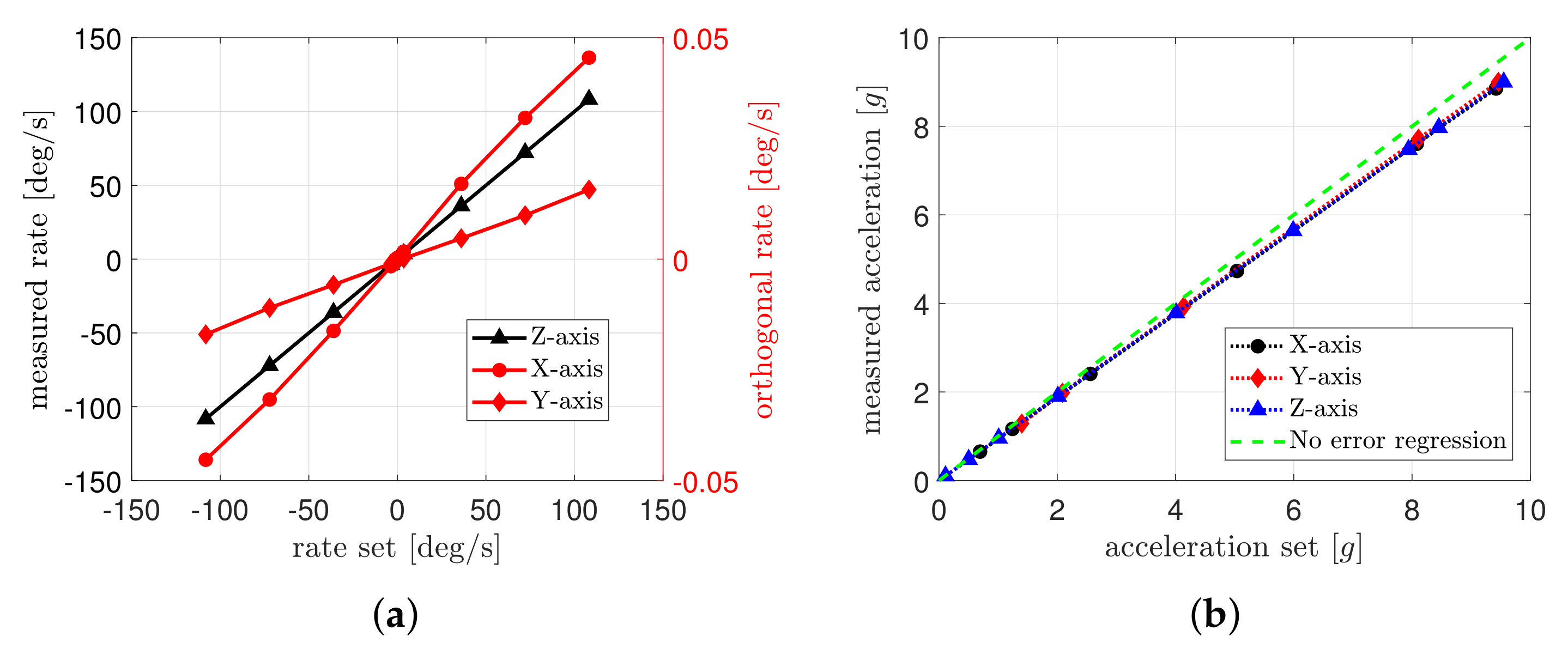
4.1. Gyroscope
4.2. Inertial Measurement Unit
4.3. Inclinometer
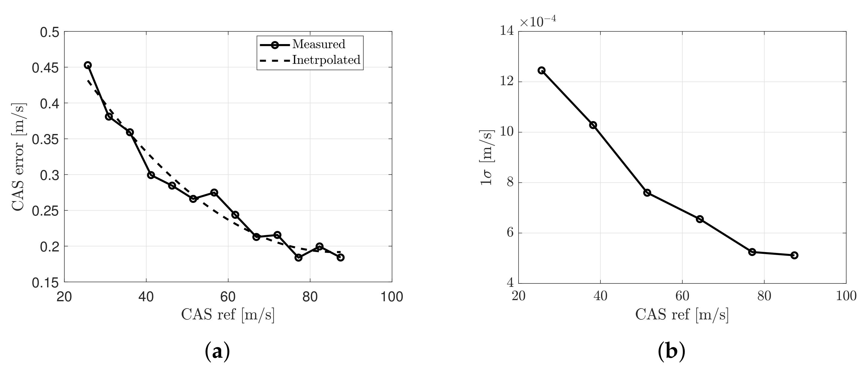
4.4. Calibrated Airspeed
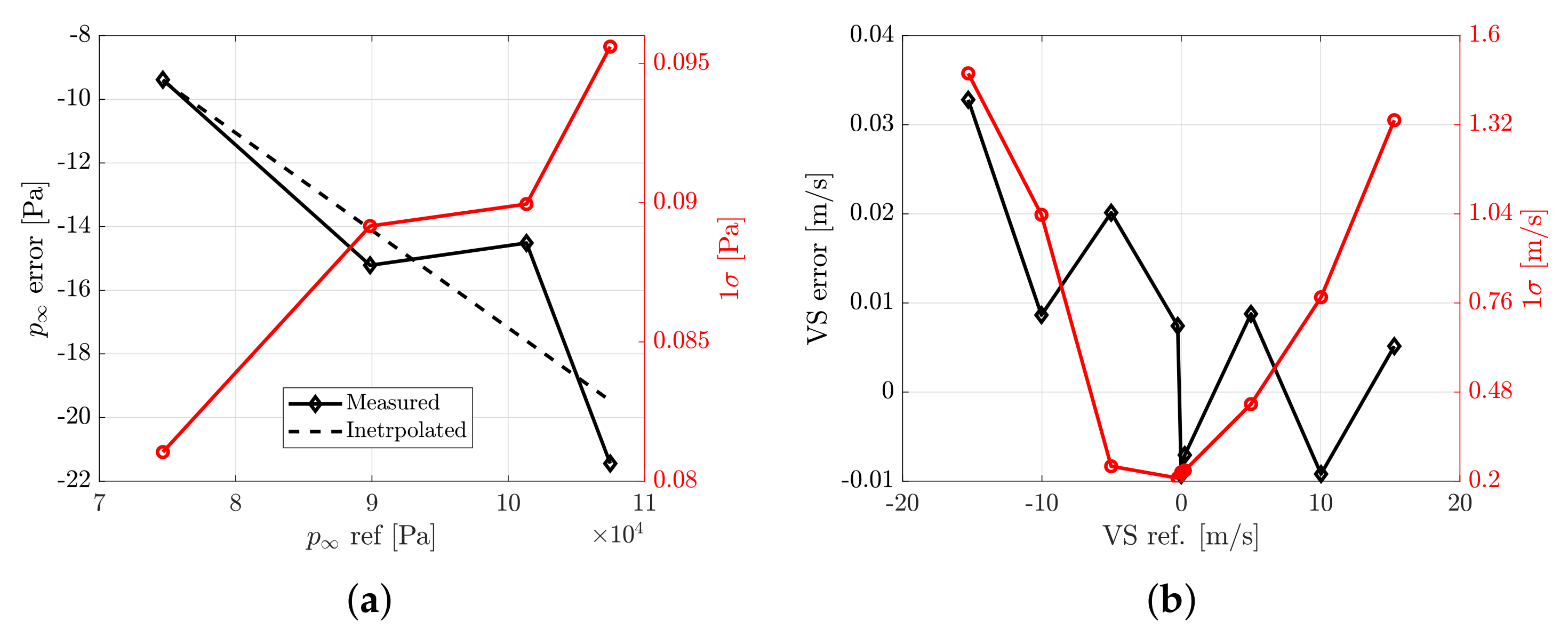
4.5. Altitude
4.6. Vertical Speed
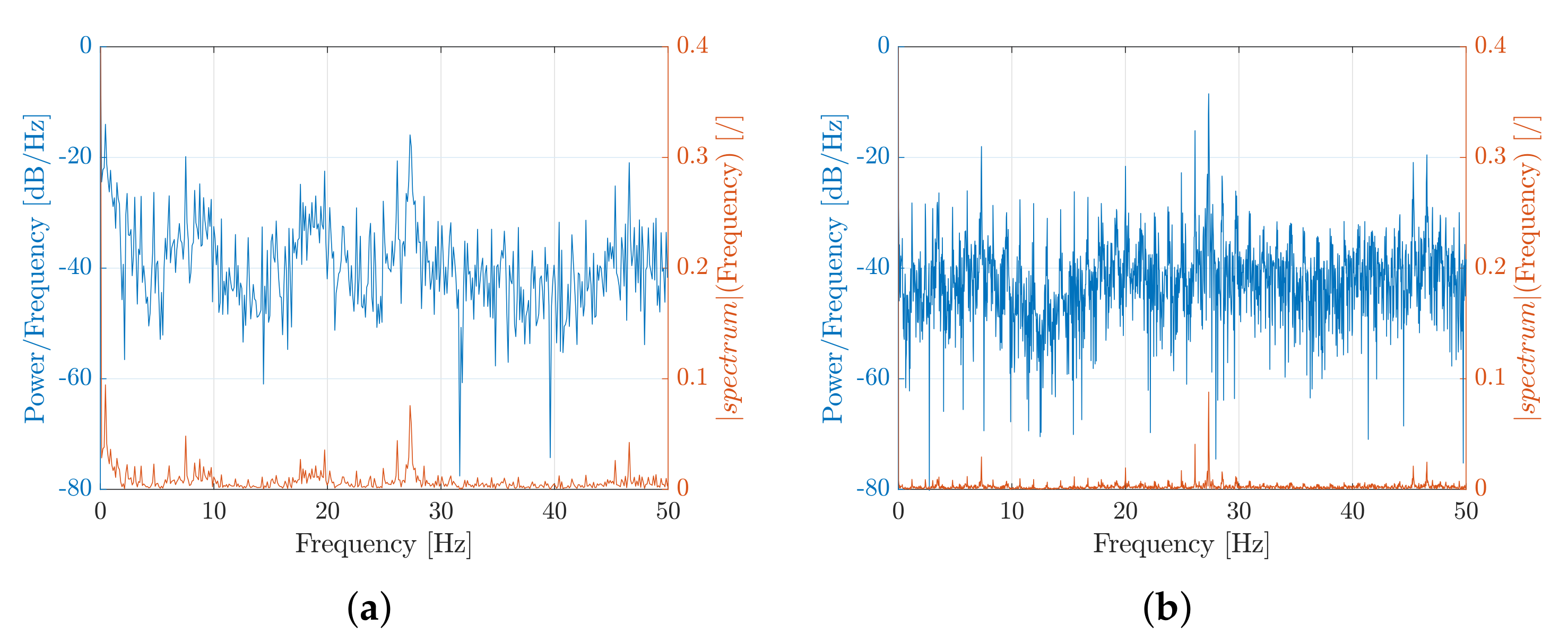
4.7. True Airspeed
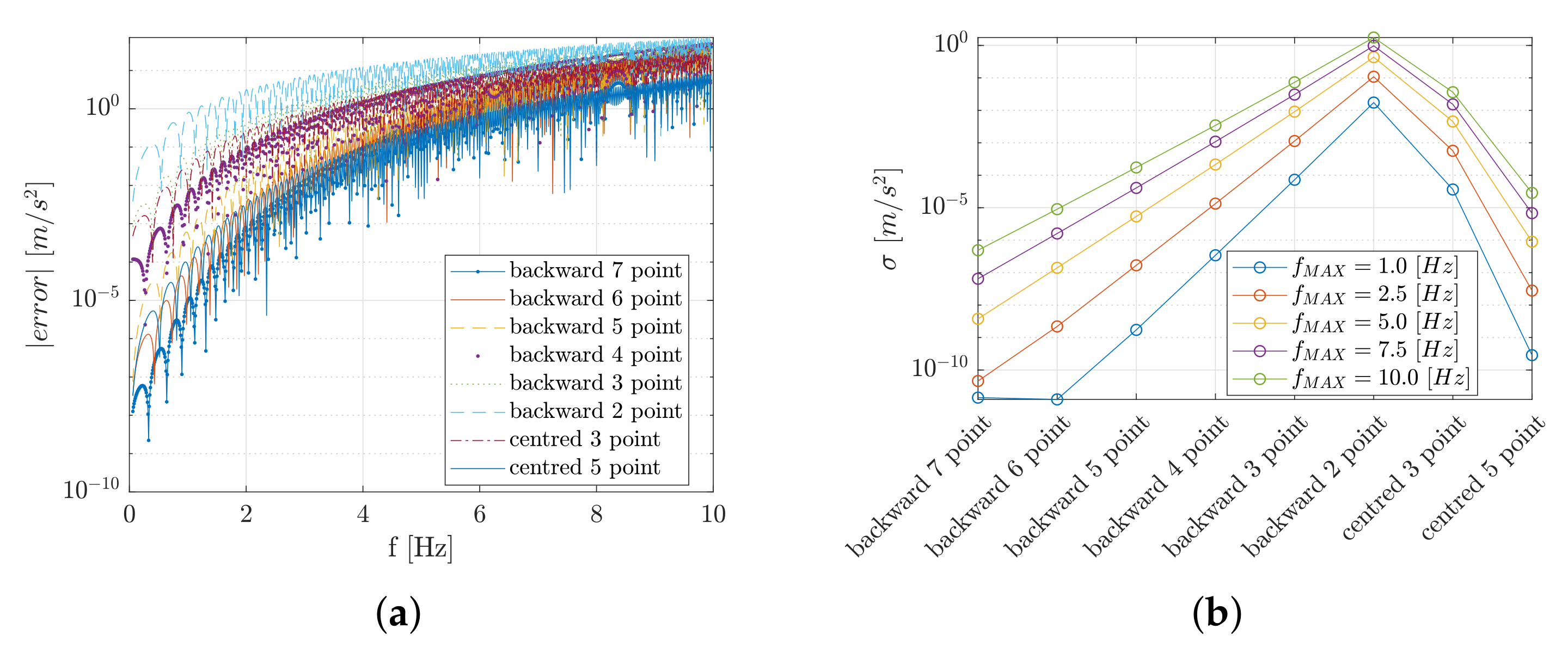
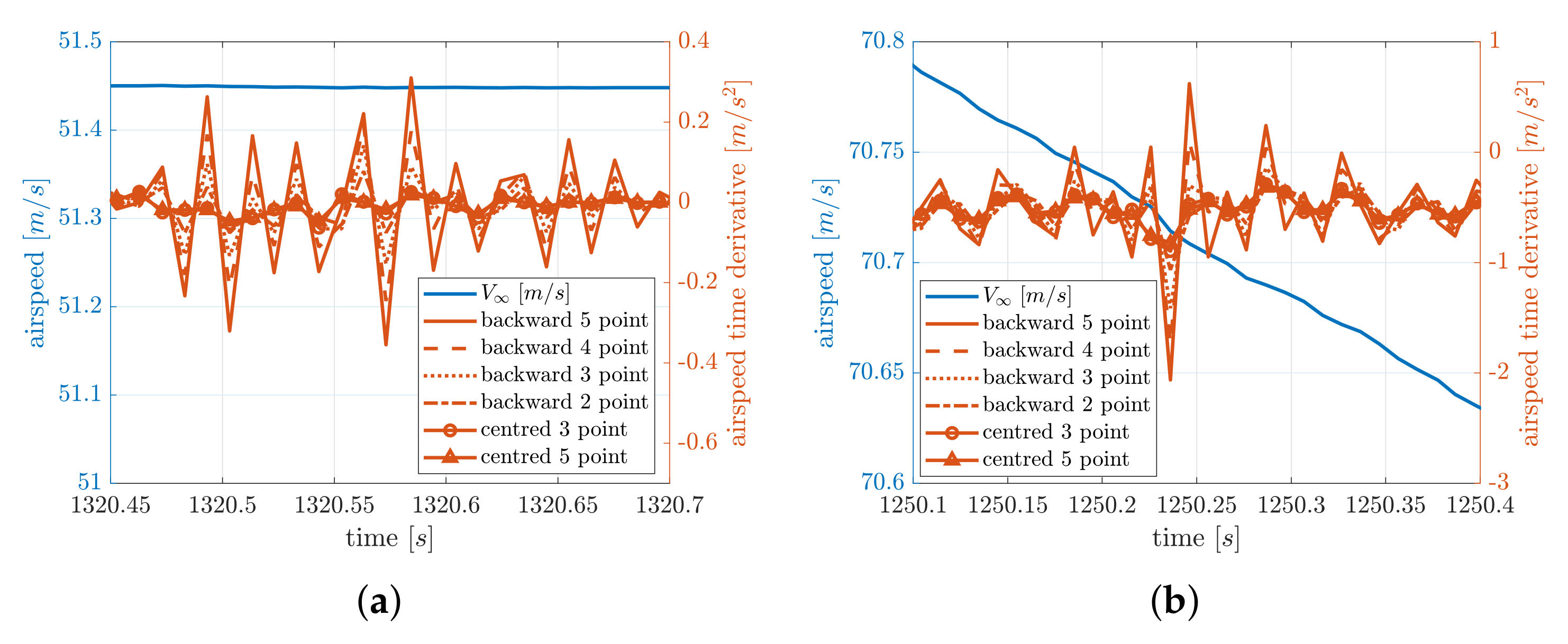
4.8. Time Derivative of the Airspeed
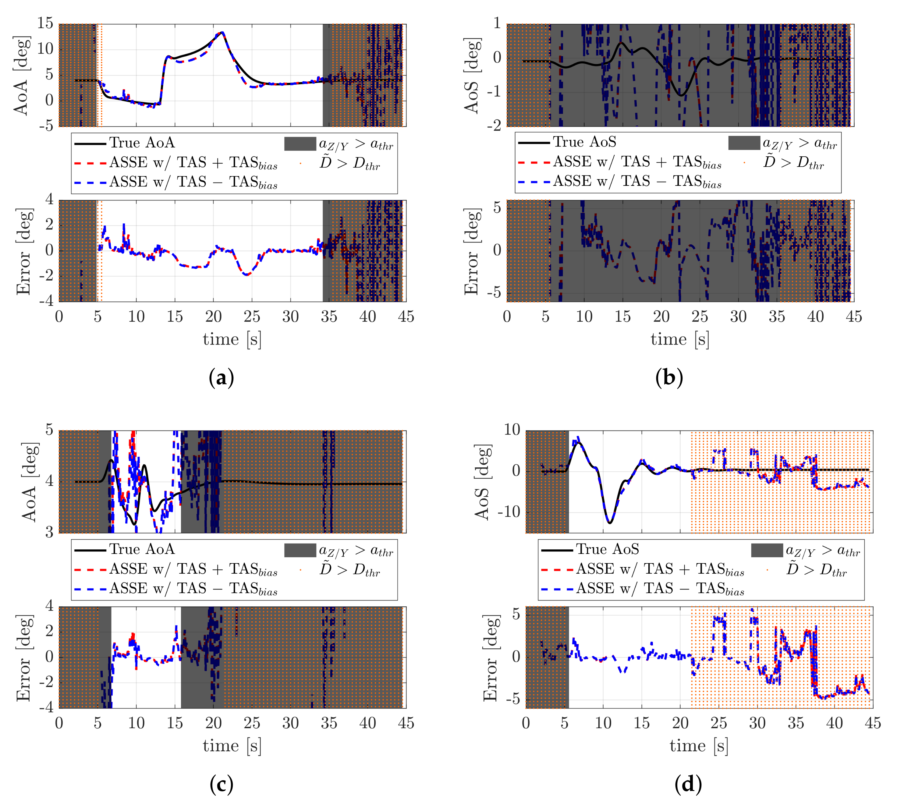
5. TRL 5 ASSE Verification
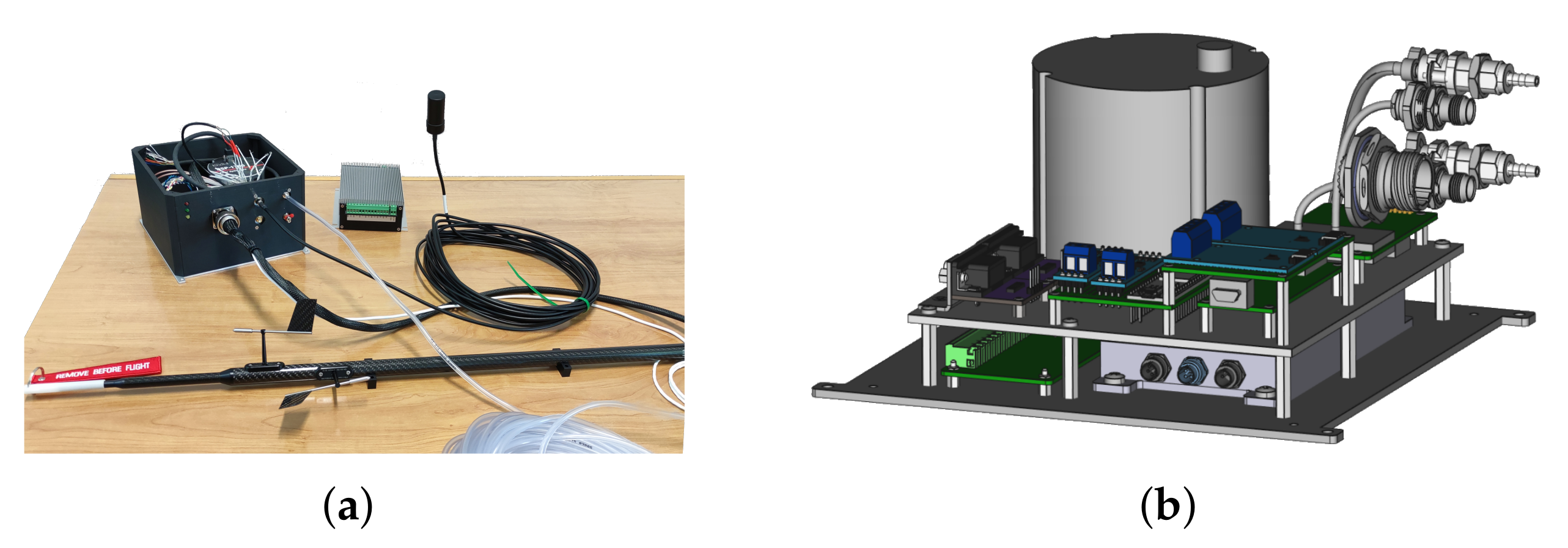
5.1. Integration Verification
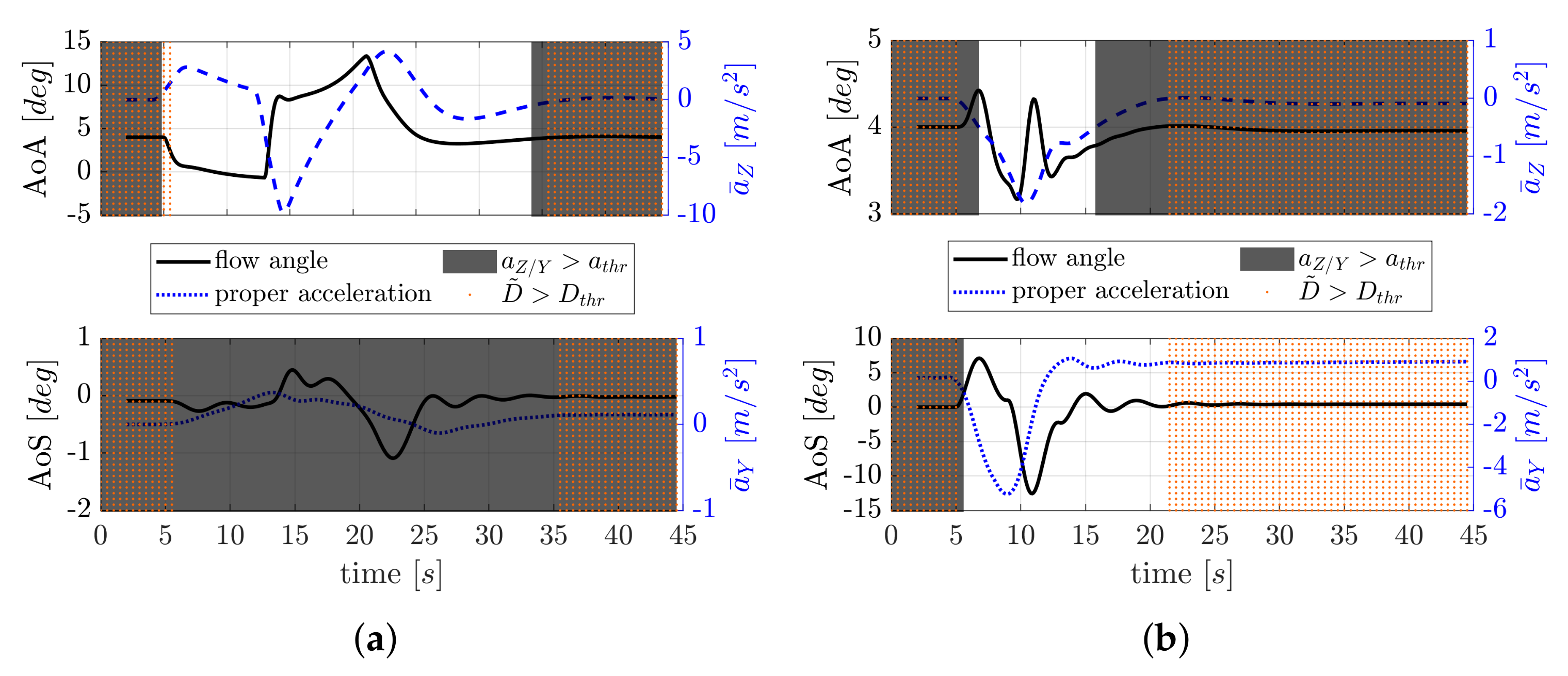
5.2. Verification by Simulation
6. Conclusions
Author Contributions
Funding
Conflicts of Interest
Abbreviations
| A/C | Aircraft |
| ADAHRS | Air Data System, Attitude and Heading Reference System |
| AHRS | Attitude and Heading Reference System |
| ADC | Air Data Computer |
| ADS | Air Data System or Sub-system |
| AoA | Angle-of-Attack |
| AoS | Angle-of-Sideslip |
| ASSE | Angle-of-Attack and -Sideslip Estimator |
| CAS | Calibrated Airspeed |
| FOG | Fibre Optical Gyroscope |
| GNSS | Global Navigation Satellite System |
| IMU | Inertial Measurement Unit |
| LRU | Line Replaceable Unit |
| MFP | Multi-Function Probe |
| OAT | Outside Air Temperature |
| SAIFE | Synthetic Air Data and Inertial Reference System |
| SFP | Single-Function Probe |
| SL | Sea level |
| SS | Synthetic Sensor |
| TAS | True Airspeed |
| TAT | Total Air Temperature |
| TRL | Technology Readiness Level |
| UAM | Urban Air Mobility |
| UAV | Unmanned Aerial Vehicles |
| VMC | vehicle management computer |
References
- Norris, G. Enhanced angle-of-attack system set for 737-10 flight test. Aviat. Week Space Technol. 2021. Available online: https://aviationweek.com/shownews/dubai-airshow/enhanced-angle-attack-system-set-737-10-flight-tests (accessed on 30 November 2021).
- SAE International. Minimum Performance Standards, for Angle of Attack (aoa) and Angle of Sideslip (AOS); SAE International: Warrendale, PA, USA, 2019. [Google Scholar]
- Vitale, A.; Corraro, F.; Genito, N.; Garbarino, L.; Verde, L. An Innovative Angle of Attack Virtual Sensor for Physical-Analytical Redundant Measurement System Applicable to Commercial Aircraft. Adv. Sci. Technol. Eng. Syst. J. 2021, 6, 698–709. [Google Scholar] [CrossRef]
- Ariante, G.; Ponte, S.; Papa, U.; Del Core, G. Estimation of Airspeed, Angle of Attack, and Sideslip for Small Unmanned Aerial Vehicles (UAVs) Using a Micro-Pitot Tube. Electronics 2021, 10, 2325. [Google Scholar] [CrossRef]
- Prem, S.; Sankaralingam, L.; Ramprasadh, C. Pseudomeasurement-aided estimation of angle of attack in mini unmanned aerial vehicle. J. Aerosp. Inf. Syst. 2020, 17, 603–614. [Google Scholar] [CrossRef]
- Valasek, J.; Harris, J.; Pruchnicki, S.; McCrink, M.; Gregory, J.; Sizoo, D.G. Derived angle of attack and sideslip angle characterization for general aviation. J. Guid. Control. Dyn. 2020, 43, 1039–1055. [Google Scholar] [CrossRef]
- Lerro, A.; Battipede, M.; Gili, P.; Ferlauto, M.; Brandl, A.; Merlone, A.; Musacchio, C.; Sangaletti, G.; Russo, G. The clean sky 2 MIDAS project—An innovative modular, digital and integrated air data system for fly-by-wire applications. In Proceedings of the 2019 IEEE 6th International Workshop on Metrology for AeroSpace (MetroAeroSpace), Turin, Italy, 19–21 June 2019; Volume 1, pp. 714–719. [Google Scholar] [CrossRef]
- Gertler, J. Analytical redundancy methods in fault detection and isolation - survey and synthesis. IFAC Proc. Vol. 1991, 24, 9–21. [Google Scholar] [CrossRef]
- Perhinschi, M.; Campa, G.; Napolitano, M.; Lando, M.; Massotti, L.; Fravolini, M. Modelling and simulation of a fault-tolerant flight control system. Int. J. Model. Simul. 2006, 26, 1–10. [Google Scholar] [CrossRef]
- Pouliezos, A.D.; Stavrakakis, G.S. Analytical Redundancy Methods; Springer: Amsterdam, The Netherlands, 1994; Volume 12, pp. 93–178. [Google Scholar] [CrossRef]
- Rhudy, M.B.; Fravolini, M.L.; Porcacchia, M.; Napolitano, M.R. Comparison of wind speed models within a Pitot-free airspeed estimation algorithm using light aviation data. Aerosp. Sci. Technol. 2019, 86, 21–29. [Google Scholar] [CrossRef]
- Eubank, R.; Atkins, E.; Ogura, S. Fault detection and fail-safe operation with a multiple-redundancy air-data system. In AIAA Guidance, Navigation, and Control Conference; American Institute of Aeronautics and Astronautics: Reston, VA, USA, 2010; pp. 1–14. [Google Scholar] [CrossRef] [Green Version]
- Lu, P.; Van Eykeren, L.; Van Kampen, E.J.; Chu, Q. Air data sensor fault detection and diagnosis with application to real flight data. In AIAA Guidance, Navigation, and Control Conference; AIAA SciTech Forum: Reston, VA, USA, 2015; pp. 1–18. [Google Scholar] [CrossRef]
- Komite Nasional Keselamatan Transportasi Republic of Indonesia. Aircraft Accident Investigation Report - PT. Lion Mentari Airlines Boeing 737-8 (MAX). KNKT.18.10.35.04. 2018. Available online: http://knkt.dephub.go.id/knkt/ntsc_aviation/baru/2018-035-PK-LQPFinalReport.pdf (accessed on 30 November 2021).
- European Aviation Safety Agency. Easy Access Rules for Unmanned Aircraft Systems; EASA: Cologne, Germany, 2015. [Google Scholar]
- European Aviation Safety Agency. Proposed Means of Compliance with the Special Condition VTOL; MOC SC-VTOL; Issue 1; EASA: Cologne, Germany, 2020. [Google Scholar]
- Estrada, M.A.R.; Ndoma, A. The uses of unmanned aerial vehicles—UAV’s- (or drones) in social logistic: Natural disasters response and humanitarian relief aid. Procedia Comput. Sci. 2019, 149, 375–383. [Google Scholar] [CrossRef]
- Radoglou-Grammatikis, P.; Sarigiannidis, P.; Lagkas, T.; Moscholios, I. A compilation of UAV applications for precision agriculture. Comput. Networks 2020, 172, 107148. [Google Scholar] [CrossRef]
- Baniasadi, P.; Foumani, M.; Smith-Miles, K.; Ejov, V. A transformation technique for the clustered generalized traveling salesman problem with applications to logistics. Eur. J. Oper. Res. 2020, 285, 444–457. [Google Scholar] [CrossRef]
- Dendy, J.; Transier, K. Angle-of-Attack Computation Study; Technical Report AFFDL-TR-69-93; Air Force Flight Dynamics Laboratory: Wright-Patterson AFB, OH, USA, 1969. [Google Scholar]
- Freeman, D.B. Angle of Attack Computation System; Technical Report AFFDL-TR-73-89; Air Force Flight Dynamics Laboratory: Wright-Patterson AFB, OH, USA, 1973. [Google Scholar]
- Rohloff, T.J.; Whitmore, S.A.; Catton, I. Air data sensing from surface pressure measurements using a neural network method. AIAA J. 1998, 36, 2094–2101. [Google Scholar] [CrossRef]
- Samara, P.A.; Fouskitakis, G.N.; Sakellariou, J.S.; Fassois, S.D. Aircraft angle-of-attack virtual sensor design via a functional pooling narx methodology. IEEE Eur. Control. Conf. 2003, 1, 1816–1821. [Google Scholar] [CrossRef]
- Wise, K.A. Computational Air Data System for Angle-of-Attack and Angle-of-Sideslip. U.S. Patent 6,928,341 B2, 2005. [Google Scholar]
- Langelaan, J.W.; Alley, N.; Neidhoefer, J. Wind field estimation for small unmanned aerial vehicles. J. Guid. Control. Dyn. 2011, 34, 1016–1030. [Google Scholar] [CrossRef]
- Lu, P.; Van Eykeren, L.; van Kampen, E.; de Visser, C.C.; Chu, Q.P. Adaptive three-step kalman filter for air data sensor fault detection and diagnosis. J. Guid. Control. Dyn. 2016, 39, 590–604. [Google Scholar] [CrossRef] [Green Version]
- Lerro, A.; Brandl, A.; Gili, P. Model-free scheme for angle-of-attack and angle-of-sideslip estimation. J. Guid. Control. Dyn. 2021, 44, 595–600. [Google Scholar] [CrossRef]
- Lerro, A.; Brandl, A.; Gili, P.; Pisani, M. The SAIFE Project: Demonstration of a Model-Free Synthetic Sensor for Flow Angle Estimation. In Proceedings of the 2021 IEEE 8th International Workshop on Metrology for AeroSpace (MetroAeroSpace), Naples, Italy, 23–25 June 2021; pp. 98–103. [Google Scholar] [CrossRef]
- Lacondemine, X.; Barbier, D. In-Flight Demonstration of a LiDAR Based Air Data System DANIELA Project. In Proceedings of the Sixth European Aeronautics Days (Aerodays), Madrid, Spain, 30 March–1 April 2011. [Google Scholar]
- Lerro, A. Survey of certifiable air data systems for urban air mobility. In Proceedings of the 2020 AIAA/IEEE 39th Digital Avionics Systems Conference (DASC), San Antonio, TX, USA, 11–15 October 2020; pp. 1–10. [Google Scholar] [CrossRef]
- Schmidt, D. Modern Flight Dynamics; McGraw-Hill: New York, NY, USA, 2011. [Google Scholar]
- Etkin, B.; Reid, L. Dynamics of Flight: Stability and Control, 3rd ed.; Wiley: Hoboken, NJ, USA, 1995. [Google Scholar]
- Lerro, A.; Brandl, A.; Gili, P. Neural network techniques to solve a model-free scheme for flow angle estimation. In Proceedings of the 2021 International Conference on Unmanned Aircraft Systems (ICUAS), Athens, Greece, 15–18 June 2021; pp. 1187–1193. [Google Scholar] [CrossRef]
- Lerro, A. Physics-based modelling for a closed form solution for flow angle Estimation. Adv. Aircr. Spacecr. Sci. 2021, 8, 273–287. [Google Scholar] [CrossRef]
- Marquardt, D.W. An algorithm for least-squares estimation of nonlinear parameters. J. Soc. Ind. Appl. Math. 1963, 11, 431–441. [Google Scholar] [CrossRef]
- Lerro, A.; Musacchio, C. Preliminary definition of metrological guidelines for synthetic sensor verification. In Proceedings of the 2020 IEEE 7th International Workshop on Metrology for AeroSpace (MetroAeroSpace), Pisa, Italy, 22–24 June 2020; pp. 187–192. [Google Scholar] [CrossRef]
- Pisani, M.; Astrua, M. The new INRIM rotating encoder angle comparator (REAC). Meas. Sci. Technol. 2017, 28, 045008. [Google Scholar] [CrossRef]
- Pisani, M.; Astrua, M.; Iafolla, V.; Santoli, F.; Lucchesi, D.; Lefevre, C.; Lucente, M. On-ground actuator calibration for ISA—BepiColombo. In Proceedings of the 2015 IEEE Metrology for Aerospace (MetroAeroSpace), Benevento, Italy, 4–5 June 2015; pp. 312–317. [Google Scholar] [CrossRef]
- Chung, T.J. Solution methods of finite difference equations. In Computational Fluid Dynamics; Cambridge University Press: Cambridge, UK, 2002; pp. 63–105. [Google Scholar] [CrossRef]


| Mean | Error | 5 Point Backward | 4 Point Backward | 3 Point Backward | 2 Point Backward | 5 Point Centred | 3 Point Centred |
|---|---|---|---|---|---|---|---|
| 0.01 m s−2 | 0.12 | 0.08 | 0.06 | 0.04 | 0.03 | 0.03 | |
| −0.51 m s−2 | 0.35 | 0.28 | 0.21 | 0.13 | 0.11 | 0.09 | |
| −1.00 m s−2 | 0.69 | 0.56 | 0.40 | 0.25 | 0.23 | 0.18 | |
| 0.01 m s−2 | 0.23 | 0.17 | 0.12 | 0.08 | 0.07 | 0.06 | |
| −0.51 m s−2 | 0.67 | 0.51 | 0.37 | 0.23 | 0.20 | 0.17 | |
| −1.00 m s−2 | 1.15 | 0.91 | 0.72 | 0.46 | 0.41 | 0.35 | |
| 0.01 m s−2 | 0.35 | 0.25 | 0.18 | 0.12 | 0.11 | 0.09 | |
| −0.51 m s−2 | 1.52 | 1.21 | 0.95 | 0.58 | 0.38 | 0.31 | |
| −1.00 m s−2 | 3.11 | 2.55 | 2.00 | 1.24 | 0.76 | 0.62 |
| Test # | TAS | a | Flow Angle Ref. (AoA, AoS) | Flow Angle Meas. AoA, AoS | ||
|---|---|---|---|---|---|---|
| 1 | 10 | 1 | N/A, | N/A, | ||
| 2 | 10 | 2 | N/A, | N/A, | ||
| 3 | 10 | N/A, | N/A, | |||
| 4 | 10 | N/A, | N/A, | |||
| 5 | 10 | , N/A | , N/A | |||
| 6 | 10 | , N/A | , N/A | |||
| 7 | 10 | 1 | , N/A | , N/A |
| Test # | TAS | Attitudes (Pitch, Roll) | Flow Angle Ref. (AoA, AoS) | Flow Angle Meas. AoA, AoS | |
|---|---|---|---|---|---|
| 8 | 10 | 96, 0 | N/A, | N/A, | |
| 9 | 10 | 102, 0 | N/A, | N/A, | |
| 10 | 10 | 114, 0 | N/A, | N/A, | |
| 11 | 10 | 0, 84 | , N/A | , N/A | |
| 12 | 10 | 0, 78 | , N/A | , N/A | |
| 13 | 10 | 0, 66 | , N/A | , N/A |
| Flow Angle | ASSE Exclusion Criteria | Mean Error | Max Abs. Error | Error | Error |
|---|---|---|---|---|---|
| AoA | OR | −0.19 | 3.02 | 0.60 | 1.66 |
| 0.18 | 3.02 | 0.61 | 1.67 | ||
| AoS | OR | 0.04 | 2.52 | 0.41 | 1.74 |
| −0.52 | 5.80 | 2.11 | 4.73 |
Publisher’s Note: MDPI stays neutral with regard to jurisdictional claims in published maps and institutional affiliations. |
© 2022 by the authors. Licensee MDPI, Basel, Switzerland. This article is an open access article distributed under the terms and conditions of the Creative Commons Attribution (CC BY) license (https://creativecommons.org/licenses/by/4.0/).
Share and Cite
Lerro, A.; Gili, P.; Pisani, M. Verification in Relevant Environment of a Physics-Based Synthetic Sensor for Flow Angle Estimation. Electronics 2022, 11, 165. https://doi.org/10.3390/electronics11010165
Lerro A, Gili P, Pisani M. Verification in Relevant Environment of a Physics-Based Synthetic Sensor for Flow Angle Estimation. Electronics. 2022; 11(1):165. https://doi.org/10.3390/electronics11010165
Chicago/Turabian StyleLerro, Angelo, Piero Gili, and Marco Pisani. 2022. "Verification in Relevant Environment of a Physics-Based Synthetic Sensor for Flow Angle Estimation" Electronics 11, no. 1: 165. https://doi.org/10.3390/electronics11010165
APA StyleLerro, A., Gili, P., & Pisani, M. (2022). Verification in Relevant Environment of a Physics-Based Synthetic Sensor for Flow Angle Estimation. Electronics, 11(1), 165. https://doi.org/10.3390/electronics11010165