Abstract
This study describes a method for classifying electrocorticograms (ECoGs) based on motor imagery (MI) on the brain–computer interface (BCI) system. This method is different from the traditional feature extraction and classification method. In this paper, the proposed method employs the deep learning algorithm for extracting features and the traditional algorithm for classification. Specifically, we mainly use the convolution neural network (CNN) to extract the features from the training data and then classify those features by combing with the gradient boosting (GB) algorithm. The comprehensive study with CNN and GB algorithms will profoundly help us to obtain more feature information from brain activities, enabling us to obtain the classification results from human body actions. The performance of the proposed framework has been evaluated on the dataset I of BCI Competition III. Furthermore, the combination of deep learning and traditional algorithms provides some ideas for future research with the BCI systems.
1. Introduction
Brain–computer interface (BCI) is a state-of-the-art technology serving as a direct communication pathway between a human brain and an external device. BCI systems can provide communication and control capabilities to humans without depending on the brain’s normal output pathways of peripheral nerves and muscles. BCI systems translate neuronal activities into user commands, messages, or other signals [1,2].
BCI systems based on sensorimotor rhythms are known as motor imagery (MI) BCI systems [2]. Sensorimotor rhythms include alpha (8–13 Hz) and beta (14–26 Hz) frequency bands [3,4]. When a human imagines a motor action without any actual movement, the power of alpha and beta rhythms can decrease or increase in the sensorimotor cortices over the contralateral hemisphere and the ipsilateral hemisphere; this phenomenon is called event-related desynchronization/synchronization (ERD/ERS) [5,6]. The imagination of motor tasks can be decoded to user intent by MI-based BCI systems [7]. Figure 1 illustrates the block diagram of BCI systems for MI classification. The complete scheme includes three main stages. In the first stage, the biomedical signal can be acquired from the users. Various kinds of brain signals have been used as the basis for interpreting the intentions of users. BCI records brain activities through non-invasive and invasive modalities [8]. The most common types of signals include electrophysiological brain activity acquired over the scalp electroencephalogram (EEG), electrophysiological brain activity recorded beneath the skull electrocorticogram (ECoG), and electrophysiological brain activity acquired from within the parenchyma local field potentials (LFPs) and single-neuron action potentials (single units) [9]. All of these major modalities for BCI record microvolt-level extracellular potentials generated by neurons in the cortical layers [10]. Non-invasive techniques such as EEG have been widely used in many important BCI systems, including two-dimensional and three-dimensional BCI control [11,12]. Compared with EEG, invasive techniques such as ECoG provide superior signal quality, higher temporal and spatial resolution, broader bandwidth, higher amplitude, better signal-to-noise ratio (SNR), and lower vulnerability to artifacts such as blinks and eye movement [13]. In the second stage, the signal processing procedure converts digitized signals into commands that operate an output device [11,14,15] (e.g., industrial robot arms, wheelchairs, quadcopters). The signal processing stage, which includes feature extraction and feature translation, is the main component of the entire system. In the third stage, brain activities can be translated into control signals that drive an output device [16,17].
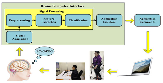
Figure 1.
The block diagram of BCI systems for MI classification. The written informed consent has been obtained from the individual for the publication of his identifiable image.
Brain functional activities associated with cognitive and behavioral events can be analyzed from the signal processing stage to classify different mental tasks to assess the performance of MI-based BCI systems [1]. How to effectively learn representations of brain activities is a key point of BCI systems. To date, machine learning technology powers many aspects of brain signal analysis. Conventional machine learning techniques were limited in their ability to process natural data in their raw form to obtain hand-designed features [18]. Traditional brain signal analysis begins with preprocessing, and then hand-crafted feature representation can be extracted. Finally, extracted feature vectors are fed into classifiers to classify different MI tasks. Many individuals or combined measures have been applied to brain activity analyses, such as band power, power spectral density, common spatial patterns, wavelet transform, autoregressive models, local binary pattern operators, and nonlinear measures (e.g., approximate entropy, sample entropy, fractal dimension, fractal intercept, and lacunarity) [1,13,18,19,20,21,22,23,24,25,26,27,28,29]. Because brain functional activities exhibit dynamic, transient, and non-stationary characteristics, acquisition signals contain numerous noises. The hand-crafted features may result in some degree of information loss during the process of feature extraction. Deep neural networks allow the system to input features containing raw spatial information, and an appropriate componential structure can be applied to learn distributed representations of data with multiple layers of extraction to make optimal classifications. Therefore, we explore the capabilities of deep-learning methods for modeling cognitive events from brain activities.
Although deep neural networks have attracted enthusiastic interest within large-scale image recognition, video recognition, and natural language processing, they remain relatively unexplored in MI-based BCI systems [30,31,32]. One of the main reasons is that the number of samples in public MI-based datasets is limited, thus making such data less adequate for training large-scale deep neural networks with millions of parameters [33]. However, the advantages of deep neural networks over traditional brain activity analyses begin to appear when the scale of datasets becomes very large or the dimension of samples becomes very high. Nevertheless, convolutional neural network (CNN), deep belief networks (DBN), and recurrent neural networks (RNN) have been employed to learn representations from EEG [33,34,35,36,37]. Li et al. (2017) developed a new neuroscience-motivated parametric CNN, which was based on parameterized convolutional filters, to consider the analysis of EEG to understand the underlying features related to the classification. Relevant experimental results showed that the proposed model outperforms conventional CNN architectures and all compared classification methods [34]. A DBN formed by a plurality of restricted Boltzmann machines (RBM) has been used to extract EEG features, and each RBM can be trained greedily and unsupervised. The performance of the proposed algorithm can achieve a 4–6% accuracy increase compared to other classifiers [35]. Long short-term memory (LSTM) was used to learn features from EEG, and then the dense layer was used for classification to obtain higher average accuracies in comparison with the conventional techniques [36]. CNN and LSTM networks were utilized to extract spatial, spectral, and temporal invariant representations from EEG data. Empirical evaluation of the cognitive load classification task demonstrated a 6.4% accuracy increase over current state-of-the-art approaches [33]. CNN and LSTM networks are employed to extract spatial and temporal patterns from EEG data, and deep forest models are used in conjunction to obtain a stronger classifier [37].
In recent years, CNN has been gradually applied to identify MI tasks in EEG-based BCI systems. The key challenge in correctly identifying MI tasks from acquired brain signals is constructing a model that is sufficiently robust for analyses of signals in time, frequency, and space. Numerous attempts have been made to improve the design of CNN architecture in a bid to achieve better performance. The convolutional neural network, which combines artificial neural networks and deep learning, is a special type of deep neural network. Its connection between neurons can take advantage of local connection architecture and shared weights. CNN contains fewer connections and parameters. The computational complexity of the network can thus be significantly reduced. CNN, which has a structure similar to biological neural networks, is more suitable for the analysis and processing of brain activities. We propose a novel approach to learning representations from ECoG that relies on deep learning with a gradient boosting algorithm to inspire state-of-the-art MI classification.
In this study, we propose an algorithm to learn representations of brain activities associated with MI depending on deep learning and to classify different MI tasks for ECoG-based BCI systems. The remainder of this paper is organized as follows. Section 2 describes the experimental dataset. The methods are introduced in Section 3. Section 4 presents the results. Finally, discussions and conclusions are summarized at the end of this paper.
2. ECoG Dataset
The experimental data are obtained from the dataset I of the BCI Competition III, which includes one subject with focal epilepsy. This is the only dataset in BCI Competitions for motor imagery based on ECoG recordings. Although the ECoG data were selected from one subject, the subdural electrode arrays were planted within the cortex of the subject suffering from focal epilepsy for one to two weeks. The patient cannot focus on MI for a long time due to needing some days to recover after the implantation surgery. It is impossible to conduct a long-time experiment, and therefore, only a small amount of data could be recorded. During the experiment, the recording structure might experience slight changes concerning electrode positions and impedances. Brain activities exhibit different states concerning motivation or fatigue across time. Thus, the experimental design of MI-based BCI systems is very challenging [38].
The experimental procedure shows that the training and test trials are recorded from two different days with an approximately one-week interval. During the BCI experiment, the patient, facing a monitor, is seated in a bed and is asked to repeatedly perform an imagined movement of either the left small finger or the tongue. The 8 × 8 platinum electrode grid is implanted on the contralateral (right) motor cortex of the patient’s right hemisphere to record ECoG data. All ECoG data are recorded with 64 active electrodes. The locations of the primary motor cortex are shown in Figure 2a. Figure 2b depicts the positions of 64 channels. All recording activities are performed with a sampling rate of 1000 Hz. The ECoG dataset consists of a training dataset and a test dataset. The imagination duration starts with a cue that is presented in the form of a picture depicting MI tasks. Each trial is recorded for 3 s, as illustrated in Figure 2c. The recorded duration starts 0.5 s after the visual cue has ended, to avoid visually evoked potentials.
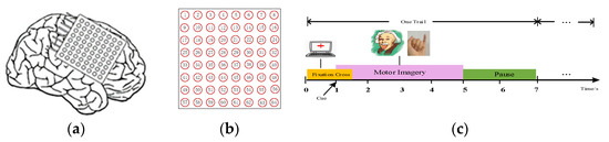
Figure 2.
(a) The locations of the primary motor cortex. (b) The positions of 64 channels. (c) The timing of the motor imagery paradigm.
3. Method
The architecture of the proposed ECoG-based BCI system is summarized in Figure 3. It contains three stages: preprocessing, unsupervised feature extraction, and classification. Different stages of the scheme are described in detail in the following sections.
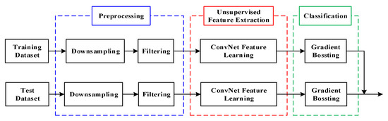
Figure 3.
The architecture of the proposed ECoG-based BCI system.
3.1. Preprocessing
The preprocessing procedure, which is crucial for denoising the signal analysis, aims to remove both high-frequency noise and low-frequency activities and subsequently to reduce the size of ECoG data and to remove artifacts. For this purpose, the ECoG is first downsampled to 100 Hz. Then, the signals are filtered between 0.5 and 30 Hz using a 5th order digital Butterworth filter. Finally, signals between 0.5 and 30 Hz exhibit the ERD/ERS phenomenon of MI tasks with reduced eye movement and electromyogram artifacts.
3.2. Feature Extraction
The purpose of this stage aims at extracting relevant features. These relevant features contain the time, frequency, and spatial characteristic properties of the ECoG signals and are suitable for MI tasks. We develop a CNN configuration to address the inherent structure of ECoG data and to obtain an optimal characterization of ECoG recordings from the right hemisphere of the brain, as well as the dynamics of the ERD/ERS phenomenon in the MI state.
CNN, which includes a feed-forward neural network that takes convolution as its core, is one of the most important concepts in deep learning. Mathematically, convolution is a function that is applied over the output of another function, and it is expressed as follows: Functions and two integrable functions over the field of real numbers. These two functions are integrated to produce a new function, which is called the convolution operation. It can be estimated as follows,
where the and functions are both variables of convolution, is the integral variable, is the amount of displacement of the function , and ““ is defined as a convolution operator. In this way, with different values of , this integral defines a new function called the convolution of the function and .
A CNN model consists of a series of different layers, including the convolutional layer, the activation layer, the pooling layer, and the fully connected layer, etc. [39,40]. The schematic of the whole MI tasks recognition course is shown in Figure 4.
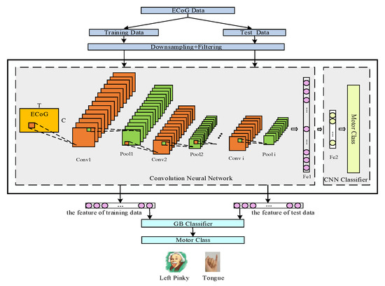
Figure 4.
The schematic of the whole MI tasks recognition course.
3.2.1. Convolutional Layer
The most important building block of a CNN is the convolutional layer, which is a linear computing layer that uses a series of convolution kernels to convolve with multi-channel input data. The convolution kernel uses a sliding window to perform small-scale weighing operations at various positions of the input ECoG data to obtain ECoG features. Feature maps can be obtained from the corresponding processing of input data.
In the convolutional layer of Caffe (convolutional architecture for fast feature embedding) [41], ECoG can be processed as follows. Given ECoG data , where is the number of recording channels, stand for sample number and denotes the total number of trials. In our method, the ECoG data first needs to be converted into Caffe-readable data, with the size of , where is the number of feature maps, and is the number of layers.
The expression of the ECoG signals after the convolution layer is,
where represents the r-th convolution kernel of the s-th layer, represents the input variable of the s-th layer, is the activation function [42], and the bias value of the network is . The mathematical expression is,
We define the size of the input convolution kernel as , where is the height of the input convolution kernel, and is the width of the kernel. The interval for convolution using the filter on the input data is , where and are the distances in the vertical and horizontal directions, respectively. The data filled on the boundary of the input data are , where and stand for the degrees of filling in the vertical and horizontal directions, respectively. The number of the output feature map of the current convolutional layer is , The output of the convolution layer is,
3.2.2. Pooling Layer
After the ECoG data pass through the convolution layer, we add one pooling layer, which is a non-linear computing layer. The goal is to subsample the input data to reduce the computational load, memory usage, and the number of parameters (thereby limiting the risk of overfitting). Similar to in convolutional layers, each neuron in a pooling layer is connected to the outputs of a limited number of neurons in the previous layer; this serves to aggregate the inputs using an aggregation function such as the max or mean. In this experiment, we use a 1 × 3 max-pooling kernel, astride of 1 × 1, and no padding; note that only the max input value in each kernel continues to the next layer, while the other inputs are dropped.
In the Caffe architecture, the change of ECoG data in the pooling layer is the same as in the convolutional layer. The definition and operation of each parameter are the same as in the convolution layer, but the calculation of ECoG data is different: one method involves convolution operation in the convolution window, while the other concerns the maximum operation in the pooling window. Specifically, the size of the input pooling kernel is , where and are the height and width of the pooling kernel. The interval for the pool using the filter on the input data is , where and represent the distances in the vertical and horizontal directions, respectively. The number of the output feature map of the current pooling layer is . The input data of the pooling layer arise from the convolutional layer, and these outputs can be expressed as
3.2.3. Fully Connected Layer
Essentially, the convolutional layers are providing a meaningful, low-dimensional, and somewhat invariant feature space. While the output from the convolutional layer could be flattened and connected to the output layer, adding a fully connected layer is a (usually) cheap way of learning non-linear combinations of these features. A fully connected layer is a linear computing layer that directly linearly transforms the input data, and we can divide the function of the fully connected layer into two parts. One is a feature extraction layer, while the other part is the final classification layer.
The fully connected layer can connect multidimensional vectors into a single feature-length vector. Each neuron in the layer is connected to all neurons in the previous layer. In the Caffe architecture, the final output of the ECoG data is
that is, , and after the data pass through the fully connected layer, the output is a single vector, and the size of the data becomes 1 × 1, where is the number of the output feature map of the current fully connected layer.
3.3. Classification
In the CNN model, the weight of the model cannot be adequately trained on a small dataset. After the last fully connected layer (as a classifier), applied to classify the test dataset, the accuracy of the CNN model can attain 89%. To make full use of the data features from the CNN model, we used gradient boosting (GB) [43] as a final classifier. GB is a machine learning technique for classification problems. It generates prediction models in the form of a set of weak predictive models. Similar to other boosting methods, such as AdaBoost and LogitBoost [44], it builds the model in a stage-wise fashion and allows optimization of any differentiable loss function.
We defined the final output data of the fully connected layer as , in which the corresponding label is represented by , and . denotes the total number of trials. The initial value of the classifier is . After iterations, the classifier will be continuously updated,
Among them, the logarithmic regression model is:
to .
The ordinary least squares (OLS) regression is used as the minimum loss function, and ; the GB algorithm based on OLS regression can be expressed as follows,
- (1)
- To calculate the gradient of the loss function along the direction of the gradient descent,
- (2)
- OLS selects the best suitable gradient that uses the weak classifier
- (3)
- Now, calculating the weight of the weak classifier,
- (4)
- To improve the generalization performance of the algorithm, the is reduced by multiplying a small per step. A strong classifier is obtained by iteration,
- (5)
- Obtaining the new logarithmic regression value, see the Formula (8)
Finally, the training and test data are input into the GB network to derive the accuracy of classification. The performance of the proposed method can be evaluated according to (13).
Additionally, we further measure the performance of deep representation by introducing the information transfer rate (ITR) [45], which can incorporate accuracy and speed in a single value. This method is calculated by,
where is the class number and is the classification accuracy.
4. Results and Discussion
4.1. Parameter Settings
In this experiment, the complete network can be divided into two parts. Feature extraction: The convolutional layers are serving the purpose of feature extraction. The CNN model captures the enhanced representation of data; hence, there is no need for feature engineering.
Classification: After feature extraction, we must classify the data into various classes, and this can be performed by using a fully connected neural network. In place of fully connected layers, we can also use a conventional classifier such as GB, k-nearest neighbor (KNN), Bayesian linear discriminate analysis (BLDA), support vector machines (SVM), and random forest (RF), etc. However, we generally end up adding GB to execute the classification procedure in this paper.
For a CNN model, the number of convolution layers and the size of the convolution kernel are important factors that affect the performance of the convolutional neural network. These parameters will directly determine the correctness of feature extraction. Under the classical LeNet-5 framework, we improved its parameter settings to extract features from the ECoG signals. The LeNet-5 consists of three convolution layers, two pooling layers, and two fully connected layers. Based on that, the total number of convolutional layers and fully connected layers is the total number of layers of the network, and there are only two fully connected layers in each experiment group.
We developed two methods of 3, 4, 5, 6, and 7 network layer numbers, and 1 × 3, 1 × 5, 1 × 7, and 1 × 9 convolution kernels, respectively, to extract features, and we also calculated the classification accuracy with a fully connected classifier. Table 1 lists the specific experimental results.

Table 1.
Classification accuracies with different CNN models.
As can be seen from the above Table 1, the CNN model classification accuracies all reached 89% when we adopted six total layers with the convolution kernel size 1 × 3, six total layers with the convolution kernel size 1 × 5, and five total layers with the convolution kernel size 1 × 7. A comparison between different algorithms was performed when placing the feature data from three of the above CNN models into the GB classifier, among which the second was the highest (92%). We chose the network structure of six layers and the convolution kernel size of 1 × 5 as a final CNN model to extract data features. Specifically, the whole CNN network and data processing course in Caffe are shown in Figure 5.
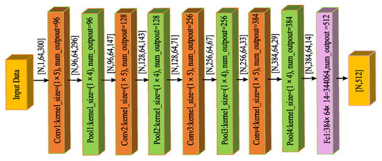
Figure 5.
The whole CNN network structure and data processing course in Caffe.
4.2. The CNN Features Visualization
The extracted CNN features further enhance the strength of ECoG signals, as shown in Figure 6. We create spectrograms from raw ECoG signals and CNN features, respectively. Figure 6a shows a raw signal during an average of all the samples in the same kind of MI tasks. Figure 6b illustrates a visual of the ECoG signal strength. Figure 6c shows the strength of CNN features. It is worth noting that Figure 6b,c are performed with the calculation of the average of all samples in the same kind of MI tasks. Ordinarily, ECoG is a low-frequency signal. These strong ECoG signals are distributed in low frequency, as shown in Figure 6b. This characteristic makes the ECoG vulnerable to being disturbed by external factors during the processing procedure. After the CNN network, we can see that the distribution of deep representation strength is wider (Figure 6c), which exactly reflects the effectiveness of the CNN network. Furthermore, two MI tasks (left pinky and tongue) in Figure 6c are more readily identifiable than in Figure 6b.
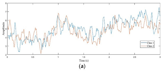
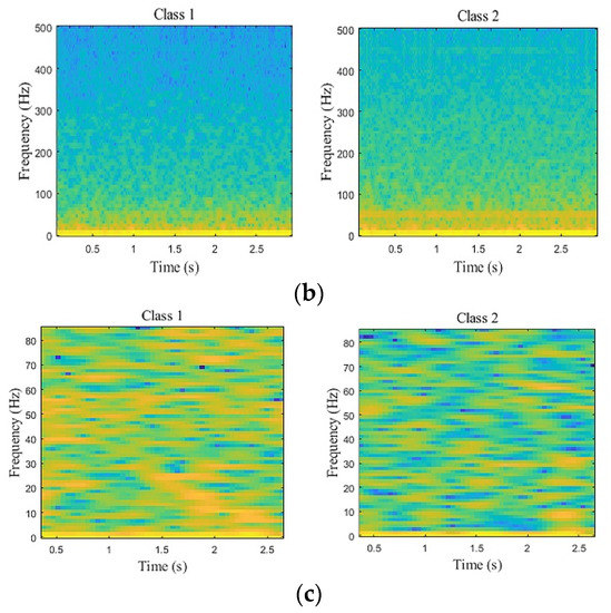
Figure 6.
Visualizing representation learned by CNN model on the ECoG. (a) Raw signal during an average of all the samples in the same kind of MI tasks. Blue and orange traces illustrate two-class motor (left pinky and tongue), respectively. (b) Generated average spectrograms from raw filtered signals shown above. (c) Generated average spectrograms from deep representation.
4.3. The Comparison of Experimental Results
In this paper, CNN works as a trainable feature extractor and GB performs as a recognizer. This hybrid model automatically extracts features from the raw ECoG data and generates the predictions. The final classification accuracy can reach 92% based on our proposed model, as shown in Figure 7a. Figure 7b,c summarize the classification performance of the different patterns of classifiers with deep representation.
Figure 7.
(a) The classification curve versus the number of iterations. (b) The classification accuracy of deep representation combined with CNN, KNN, BLDA, SVM, RF, and GB classifiers, respectively. (c) The average ITR of each trial.
The classifiers include GB, Bayesian linear discriminate analysis (BLDA), KNN, and SVM classifiers. The accuracies of different algorithms vary from 89% to 92%. The deep representation with GB classifier can achieve the best performance. Furthermore, Figure 7 also shows that deep representation can obtain higher ITR.
Finally, the algorithm proposed in this paper is compared with other methods. The competition winner got the accuracy of 91% by employing the combination features including band power, common spatial subspace decomposition (CSSD), and mean waveform mean [46]. Using the common spatial pattern (CSP) as a trainable feature extractor and with SVM performing as a classifier, its accuracy reaches 84% [47], and the goal of the CSP algorithm is to find a set of optimal spatial filters for projection and to obtain a higher resolution eigenvector. Extracting data features from the wavelet transform (WT) and using the probabilistic neural network (PNN) as a classifier can enable the accuracy of 88% [48]. The power features are extracted by relative wavelet energy (RWE), and the used PNN classifier can get an accuracy of 91.8% [49]. Xu F. et al. (2014) developed a modified s-transform (MST) algorithm, which is an improved method based on the s-transform algorithm. It may achieve 92% classification accuracy by the MST feature extraction algorithm with the GB classifier [50]. The result is shown in Table 2. The classification accuracy of the method proposed in this paper is higher than that of other references. Under the same classification accuracy, the computational complexity is higher when using the MST than the CNN. Moreover, the CNN algorithm accelerates by using GPUs, requiring less time, and running more quickly.
Table 2.
Comparison of the classification accuracy of our method with other methods.
5. Conclusions
A novel deep representation m0ethod that exploits the inherent characteristics of MI-based ECoG is introduced in this paper. The CNN algorithm is introduced to learn representation from ECoG signals, and then the deep representation is fed into the traditional GB classifier. The better classification accuracy and higher ITR demonstrate the effectiveness of the proposed combinational algorithm. Additionally, we show the performance of the system under different CNN network structures. This system can realize high-speed real-time arithmetic depend on Caffe and GPUs.
Author Contributions
Funding acquisition, J.L. (Jincheng Li); methodology, F.X., F.R. and Y.M.; project administration, J.L. (Jiancai Leng); software, Y.S., G.D. and H.L.; validation, J.L. (Jincheng Li) and Y.W.; writing—original draft, F.X., F.R., Y.M., Y.S., H.L. and Y.W.; writing—review & editing, F.X., G.D. and J.L. (Jiancai Leng). All authors have read and agreed to the published version of the manuscript.
Funding
This research received no external funding.
Acknowledgments
The project is supported in part by the National Natural Science Foundation of China under Grant No.61701270 and Grant No. 81472159, in part by the Graduate Supervisor Ability Improvement Project of Shandong under Grant No. SDYY18151, in part by the Key Research and Development Plan of Shandong Province under Grant No. 2017G006014, in part by the Natural Science Foundation of Shandong Province of China, Grant No. ZR2019MA037 and Grant No. ZR2017ZF003, in part by the Program for Youth Innovative Research Team in the University of Shandong Province in China under Grant No. 2019BSHZ003, in part by the Graduate Education and Teaching Reform Research Project of Qilu University of Technology in 2019 under Grant No. YJG19007, in part by the School-level Teaching and Research Projects of Qilu University of Technology in 2019 under Grant No. 2019yb15, and in part by the Research Leader Program of Jinan Science and Technology Bureau, Grant No. 2019GXRC061, in partby the Key Program for Research and Development of Shandong Province, China (Key Project for Science and Technology Innovation, Department and City Cooperation) (Grant 2019TSLH0315), in part by the Jinan Program for Development of Science and Technology, in part by the Jinan Program for Leaders of Science and Technology.
Conflicts of Interest
The authors declare no conflict of interest.
References
- Xu, F.Z.; Zhou, W.D.; Zhen, Y.L.; Yuan, Q.; Wu, Q. Using fractal and local binary pattern features for classification of ECoG motor imagery tasks obtained from the right brain hemisphere. Int. J. Neural. Syst. 2016, 26, 1650022. [Google Scholar] [CrossRef]
- Hamedi, M.; Salleh, S.H.; Noor, A.M. Electroencephalographic motor imagery brain connectivity analysis for BCI: A review. Neural Comput. 2016, 28, 999–1041. [Google Scholar] [CrossRef] [PubMed]
- Kim, Y.; Ryu, J.; Kim, K.K.; Took, C.C.; Mandic, D.P.; Park, C. Motor imagery classification using mu and beta rhythms of EEG with strong uncorrelated transform based complex common spatial patterns. Comput. Intel. Neurosci. 2016, 2016, 1489692. [Google Scholar] [CrossRef] [PubMed]
- Brinkman, L.; Stolk, A.; Dijkerman, H.C.; Lange, F.P.; Toni, I. Distinct roles for alpha-and beta-band oscillations during mental simulation of goal-directed actions. J. Neurosci. 2014, 34, 14783–14792. [Google Scholar]
- Pfurtscheller, G.; Sliva, F.H.L.D. Event-related EEG/MEG synchronization and desynchronization: Basic principles. Clin. Neurophsiol. 1999, 110, 1842–1857. [Google Scholar]
- Pregenzer, M.; Pfurtscheller, G. Frequency component selection for an EEG-based brain to computer Interface. IEEE. Trans. Rehabil. Eng. 1999, 7, 413–419. [Google Scholar]
- Aghaei, A.S.; Mahanta, M.S.; Plataniotis, K.N. Separable common spatio-spectral patterns for motor imagery BCI systems. IEEE. Trans. Bio-Med. Eng. 2016, 63, 15–29. [Google Scholar]
- Ortiz-Rosario, A.; Adeli, H. Brain-computer interface technologies: From signal to action. Rev. Neurosci. 2013, 24, 537–552. [Google Scholar]
- Leuthardt, E.C.; Schalk, G.; Roland, J.; Rouse, A.; Moran, D.W. Evolution of brain-computer interfaces: Going beyond classic motor physiology. Neurosurg. Focus. 2009, 27, 1–21. [Google Scholar] [CrossRef]
- Yuan, H.; He, B. Brain-computer interfaces using sensorimotor rhythms: Current state and future perspectives. IEEE. Trans. Bio-Med. Eng. 2014, 6, 1425–1435. [Google Scholar]
- Meng, J.; Zhang, S.; Bekyo, A.; Olsoe, J.; Baxter, B.; He, B. Noninvasive electroencephalogram based control of a robotic arm for reach and grasp tasks. Sci. Rep. UK 2016, 6, 38565. [Google Scholar] [CrossRef] [PubMed]
- Horki, P.; Solis-Escalante, T.; Neuper, C.; Müller-Putz, G. Combined motor imagery and SSVEP based BCI control of a 2 DoF artificial upper lmb. Med. Biol. Eng. Comput. 2011, 49, 567–577. [Google Scholar] [CrossRef] [PubMed]
- Xu, F.Z.; Zhen, Y.; Yuan, Q. Classification of motor imagery tasks for electrocorticogram based brain-computer interface. Biomed. Eng. Lett. 2014, 4, 149–157. [Google Scholar] [CrossRef]
- Wolpaw, J.R.; Birbaumer, N.; McFarland, D.J.; Pfurtscheller, G.; Vaughan, T.M. Brain–computer interfaces for communication and control. Clin. Neurophsiol. 2002, 113, 767–791. [Google Scholar] [CrossRef]
- Schalk, G.; Mcfarland, D.J.; Hinterberger, T.; Birbaumer, N.; Wolpaw, J.R. BCI2000: A general-purpose brain-computer interface (BCI) system. IEEE. Trans. Bio-Med. Eng. 2004, 51, 1034–1043. [Google Scholar] [CrossRef] [PubMed]
- Wang, F.; Zhang, X.; Fu, R.; Sun, G. Study of the home-auxiliary robot based on BCI. Sensors 2018, 18, 1779. [Google Scholar] [CrossRef]
- Albuquerque, V.H.C.d.; Damaševičius, R.; Garcia, N.M.; Pinheiro, P.R.; Pedro Filho, P.R. Brain computer interface systems for neurorobotics: Methods and applications. Biomed. Res. Int. 2017, 2017, 1–3. [Google Scholar] [CrossRef]
- Lecun, Y.; Bengio, Y.; Hinton, G. Deep learning. Nature 2015, 512, 436–444. [Google Scholar] [CrossRef]
- Pfurtscheller, G.; Brunner, C.; Schlögl, A.; Lopes da Silva, F.H. Mu rhythm (de) synchronization and EEG single-trial classification of different motor imagery tasks. Neuroimage 2006, 31, 153–159. [Google Scholar] [CrossRef]
- Zhao, Y.; Han, J.; Chen, Y.; Sun, H.; Chen, J.; Ke, A.; Han, Y.; Zhang, P.; Zhang, Y.; Zhou, Y.; et al. Improving generalization based onl1-norm regularization for EEG-based motor imagery classification. Front. Neurosci-Switz. 2018, 12, 272. [Google Scholar] [CrossRef]
- Lotte, F.; Guan, C. Regularizing common spatial patterns to improve BCI designs: Unified theory and new algorithms. IEEE Trans. Biomed. Eng. 2011, 58, 355–362. [Google Scholar] [CrossRef] [PubMed]
- Sharma, P.; Khan, Y.U.; Farooq, O.; Tripathi, M.; Adeli, H. A wavelet-statistical features spproach for nonconvulsive seizure detection. Clin. EEG Neurosci. 2014, 45, 274–284. [Google Scholar] [CrossRef] [PubMed]
- Sankari, Z.; Adeli, H.; Adeli, A. Wavelet coherence model for diagnosis of alzheimer Disease. Clin. EEG Neurosci. 2012, 43, 268–278. [Google Scholar] [CrossRef] [PubMed]
- Faust, O.; Acharya, U.R.; Adeli, H.; Adeli, A. Wavelet-based EEG processing for computer-aided seizure detection and epilepsy diagnosis. Seizure 2015, 26, 56–64. [Google Scholar] [CrossRef] [PubMed]
- Adeli, H.; Ghoshdastidar, S.; Dadmehr, N. A spatio-temporal wavelet-chaos methodology for EEG-based diagnosis of alzheimer’s disease. Neurosci. Lett. 2008, 444, 190–194. [Google Scholar] [CrossRef]
- Meisheri, H.; Ramrao, N.; Mitra, S. Multiclass common spatial pattern for EEG based brain computer interface with adaptive learning classifier. arXiv 2018, arXiv:1802.09046. [Google Scholar]
- Ahmadlou, M.; Adeli, H.; Adeli, A. Improved Visibility Graph Fractality with Application for the Diagnosis of Autism Spectrum Disorder. Physica A 2012, 391, 4720–4726. [Google Scholar] [CrossRef]
- Chu, Y.; Zhao, X.; Zou, Y.; Xu, W.; Han, J.; Zhao, Y. A decoding scheme for incomplete motor imagery EEG with deep belief network. Front. Neurosci-Switz. 2018, 12, 680. [Google Scholar] [CrossRef]
- Ahmadlou, M.; Adeli, H.; Adeli, A. Fractality analysis of frontal brain in major depressive disorder. Int. J. Psychophysiol. 2012, 85, 206–211. [Google Scholar] [CrossRef]
- Krizhevsky, A.; Sutskever, I.; Hinton, G.E. Imagenet classification with deep convolutional neural networks. Commun. ACM 2017, 60, 84–90. [Google Scholar] [CrossRef]
- Donahue, J.; Hendricks, L.A.; Guadarrama, S.; Rohrbach, M.; Venugopalan, S.; Saenko, K.; Darrell, T. Long-term recurrent convolutional networks for visual recognition and description. IEEE. Trans. Pattern. Anal. 2017, 39, 677–691. [Google Scholar] [CrossRef] [PubMed]
- Taylor, S.; Kim, T.; Yue, Y.; Mahler, M.; Krahe, J.; Rodriguez, A.G.; Hodgins, J.; Mattews, I. A deep learning approach for generalized speech animation. ACM Trans. Graph. 2017, 36, 1–11. [Google Scholar] [CrossRef]
- Bashivan, P.; Rish, I.; Yeasin, M.; Codella, N. Learning representations from EEG with deep recurrent-convolutional neural networks. arXiv 2015, arXiv:1511.06448. [Google Scholar]
- Li, Y.; Dzirasa, K.; Carin, L.; Carlson, D.E. Targeting EEG/LFP synchrony with neural nets. Adv. Neural Inf. Process. Syst. 2015, 30, 4620–4630. [Google Scholar]
- Frydenlund, A.; Rudzicz, F. Emotional affect estimation using video and EEG data in deep neural networks. Adva. Artif. Intell. (AI 2015) 2015, 9091, 273–280. [Google Scholar]
- Alhagry, S.; Fahmy, A.A.; El-Khoribi, R.A. Emotion recognition based on EEG using LSTM recurrent neural network. Emotion 2010, 8, 355–358. [Google Scholar] [CrossRef]
- Shen, Y.; Lu, H.; Jie, J. Classification of motor imagery EEG signals with deep learning models. In International Conference on Intelligent Science and Big Data Engineering; Springer: Cham, Switzerland, 2017; pp. 181–190. [Google Scholar]
- Lal, T.N.; Hinterberger, T.; Widman, G.; Schroder, M.; Hill, J.; Rosenstiel, W.; Elger, C.E.; Scholklpf, B.; Birbaumer, N. Methods towards invasive human brain computer interfaces. Adv. Neural Inf. Process. Syst. 2005, 17, 737–744. [Google Scholar]
- Foss, S.; Korshunov, D.; Zachary, S. Convolutions of long-tailed and subexponential distributions. J. Appl. Probab. 2009, 46, 756–767. [Google Scholar] [CrossRef][Green Version]
- Szegedy, C.; Liu, W.; Jia, Y.; Sermanet, P.; Reed, S.; Anguelov, D.; Erhan, D.; Vanhouchk, V.; Rabinovich, A. Going deeper with convolutions. In Proceedings of the IEEE Conference on Computer Vision and Pattern Recognition 2015, Boston, MA, USA, 7–12 June 2015; pp. 1–9. [Google Scholar]
- Jia, Y.; Shelhamer, E.; Donahue, J.; Karayev, S.; Long, J.; Girshick, R.; Guadarrama, S.; Darrell, T. Caffe: Convolutional architecture for fast feature embedding. In Proceedings of the ACM International Conference on Multimedi, Orlando, FL, USA, 3–7 November 2014; pp. 675–678. [Google Scholar]
- Glorot, X.; Bordes, A.; Bengio, Y. Deep sparse rectifier neural networks. In Proceedings of the International Conference on Artificial Intelligence and Statistics, Ft. Lauderdale, FL, USA, 11–13 April 2011; pp. 315–323. [Google Scholar]
- Natekin, A.; Knoll, A. Gradient boosting machines, a tutorial, Front. Neurorobotics 2013, 7, 21. [Google Scholar]
- Blagus, R.; Lusa, L. Boosting for high-dimensional two-class prediction. BMC Bioinform. 2015, 16, 1–17. [Google Scholar]
- Wang, D.; Miao, D.; Blohm, G. Multi-class motor imagery EEG decoding for brain-computer interfaces. Front. Neurosci-Switz. 2012, 6, 151. [Google Scholar] [CrossRef] [PubMed]
- Blankertz, B.; Muller, K.R.; Krusienski, D.J.; Schalk, G.; Wolpaw, J.R.; Schlogl, A.; Pfurtscheller, G.; Millan, J.R.; Schroder, M.; Pfurscheller, G.; et al. The BCI Competition. III: Validating alternative approaches to actual BCI problems. IEEE. Trans. Neural Syst. Rehabil. 2006, 14, 153–159. [Google Scholar] [CrossRef] [PubMed]
- Li, M.; Yang, J.; Hao, D.; Jia, S. ECoG recognition of motor imagery based on SVM ensemble. In Proceedings of the IEEE International Conference on Robotics & Biomimetics, Guilin, China, 19–23 December 2009; pp. 1967–1972. [Google Scholar]
- Yan, S.Y.; Guan, D.J. ECoG classification research based on wavelet variance and probabilistic neural network. AMM 2013, 380, 2280–2285. [Google Scholar] [CrossRef]
- Zhao, H.-b.; Yu, C.-y.; Liu, C.; Wang, H. ECoG-based brain-computer interface using relative wavelet energy and probabilistic neural network. In Proceedings of the International Conference on Biomedical Engineering and Informatics, Yantai, China, 16–18 October 2010. [Google Scholar]
- Xu, F.; Zhou, W.; Zhen, Y.; Yuan, Q. Classification of ECoG with modified S-Transform for brain-computer interface. J. Comput. Inform. Syst. 2014, 10, 8029–8804. [Google Scholar]


Publisher’s Note: MDPI stays neutral with regard to jurisdictional claims in published maps and institutional affiliations. |
© 2021 by the authors. Licensee MDPI, Basel, Switzerland. This article is an open access article distributed under the terms and conditions of the Creative Commons Attribution (CC BY) license (http://creativecommons.org/licenses/by/4.0/).