Robust Autoregression with Exogenous Input Model for System Identification and Predicting

Abstract

Autoregression with exogenous input (ARX) is a widely used model to estimate the dynamic relationships between neurophysiological signals and other physiological parameters. Nevertheless, biological signals, such as electroencephalogram (EEG), arterial blood pressure (ABP), and intracranial pressure (ICP), are inevitably contaminated by unexpected artifacts, which may distort the parameter estimation due to the use of the L2 norm structure. In this paper, we defined the ARX in the Lp (p ≤ 1) norm space with the aim of resisting outlier influence and designed a feasible iteration procedure to estimate model parameters. A quantitative evaluation with various outlier conditions demonstrated that the proposed method could estimate ARX parameters more robustly than conventional methods. Testing with the resting-state EEG with ocular artifacts demonstrated that the proposed method could predict missing data with less influence from the artifacts. In addition, the results on ICP and ABP data further verified its efficiency for model fitting and system identification. The proposed Lp-ARX may help capture system parameters reliably with various input and output signals that are contaminated with artifacts.

1. Introduction

In the field of linear system identification, the autoregression with exogenous input (ARX) model [1,2,3] is the most widely used linear dynamic model due to being easily implemented by L2 norm-based analytical solutions and capturing the linear relationship in various real-world systems [4]. In recent years, the ARX model has been widely applied in electroencephalogram (EEG)-related system identification [5,6], EEG network analysis [7,8,9], and brain–computer interfaces [10]. For instance, Burke and colleagues used the ARX model to combine both feature filtering and feature extraction for EEG signal processing [11]. Li and colleagues represented the dynamic variation of parameters in time-varying ARX models with a series of multiwavelet bases and applied orthogonal least squares (OLS) regression to improve the robustness of the parameter estimation, which captured the transient information of the inherent dynamics of nonstationary systems [12]. Moreover, Qidwai and colleagues developed an ARX-based dynamic model for EEG signal simulation that can be used to simulate any number of data samples from a predefined signal type (normal, preseizure and seizure) [13].

Nevertheless, applications in EEG are still limited because EEG signals are inevitably contaminated with artifacts due to eye blinks or head movement, which act similar to outliers and usually result in large effects on parameter estimation in the ARX model. Many methods have been applied to parameter estimation of neurophysiological signals, such as the general linear model (GLM) and Granger causality analysis (GCA). Yu and colleagues used GCA to estimate the effective connectivity between neurons and discussed the relationship between synchronization and effective connections [14,15]. Liao and colleagues applied a conditional GCA to evaluate the possible effective connectivity within the resting-state networks retrieved by independent component analysis (ICA) [16]. Kim and colleagues proposed a point process framework that enables GCA to be applied to point process data. Meanwhile, they evaluated the framework on real neural data and identified causal relationships between many of the recorded neurons [17]. However, most of these works paid little attention to the outlier effect, even though well-known techniques such as OLS and sparse constraint, may suppress the outlier effect to some degree [18]. Wang and colleagues proposed combining ICA with ARX to remove ocular artifacts [6]. In real applications, it is an open issue that it is cumbersome and time-consuming for users to clearly identify artifact components. Moreover, when artifacts and signals are unexpectedly represented in the same component, it is difficult to remove artifacts without distorting useful signals. Theoretically, the original ARX and its improvements are mainly structured in L2 norm space, and the L2 norm will be influenced by outliers due to its square property [19,20,21].

Recently, the Lp (p ≤ 1) norm has been introduced as a solution for the sparse signal recovery problem [22,23,24,25] and machine learning [13,22,26,27,28], in which the objectives involve Lp-norm minimization terms. These works show that the Lp method often performs better than other available methods. In addition, some previous works have proven that the Lp (p ≤ 1) norm is robust to outliers in biomedical signal processing, such as the denoising and EEG inverse problems [29,30]. In the area of clinical neurology and cognitive neuroscience, Xu and colleagues proposed a novel iterative EEG source imaging algorithm, the Lp (p ≤ 1) norm iterative sparse solution (LPISS), to localize neural electric activities effectively and precisely from scalp EEG recordings [19]. In this work, motivated by the ability of the Lp (p ≤ 1) norm to suppress the influence of outliers, we restructured the ARX model in the Lp (p ≤ 1) norm space and utilized a reasonable iteration procedure to solve this new ARX model, which is referred to as Lp-ARX. The proposed model was then evaluated under numerous conditions, which contained different outlier occurrence rates and outlier strengths for single-input and -output (SISO) and multiple-input and single-output (MISO) systems. We also evaluated the performance of Lp-ARX on real physiological data, such as EEG and arterial blood pressure (ABP).

Moreover, we have proposed the Lp-AR and Lp-GA models in our earlier works [31,32]. In essence, our former proposed Lp-AR is mainly designed for the power spectral density estimation of a single variate, and the Lp-GA was used to estimate the interactions between multiple time series. Different from Lp-AR and Lp-GA models, the designing purpose of Lp-ARX model is to capture system parameters reliably with various input and output signals that are contaminated with artifacts. The similarity between Lp-AR model, Lp-GA model, and the Lp-ARX model is that all of them can be solved by least square solution. However, the extension from Lp-AR model and Lp-GA model to Lp-ARX model is meaningful, especially for the actual data acquisition process, the proposed Lp-ARX model may provide a feasible scheme for eliminating signals contaminated with artifacts. The newly proposed Lp-ARX model is designed to suppress the influence of outliers. Though the coefficients estimation for them Lp (p ≤ 1) AR, Lp (p ≤ 1) GA and Lp (p ≤ 1) ARX used same sub-gradient strategy, the problem and objective functions for these three methods are different, resulting in different application areas.

2. Materials and Methods

2.1. SISO ARX

A SISO ARX model is usually represented as

$$y(n)={\displaystyle \sum _{i=1}^{n_a}{a}_{i}y\left(n-i\right)} +{\displaystyle \sum _{j=1}^{n_b}{b}_{j}u\left(n-n_k-j+1\right)}+e\left(n\right)$$

(1)

where $y(n)$ and $u(n)$ (n = 1, … N) are the output and input of the system, respectively, $e\left(n\right)$ is a zero-mean white Gaussian noise with variance ${\sigma }_w^2$. $a_i$ (i = 1, …, $n_a$) and $b_j$ (j = 1, …, n_b) are the model parameters for the output and input, respectively, $n_a$ and $n_b$ are the degree of the ARX model, and $n_k$ is the time delay.

Let $W={\left[a_1,a_2,\cdots ,a_{n_a},b_1,b_2,\cdots ,b_{n_b}\right]}^T$, $\psi (n)={\left[{\psi }_y\left(n\right),{\psi }_u\left(n\right)\right]}^T$, where

$${\psi }_y\left(n\right)=\left[y\left(n-1\right),\cdots ,y\left(n-n_a\right)\right]$$

(2)

$${\psi }_u\left(n\right)=\left[u\left(n-n_k\right),u\left(n-n_k-1\right),\cdots ,u\left(n-n_k-n_b+1\right)\right]$$

(3)

where ${\psi }_y\left(n\right)\in R^{1\times n_a}$ consists of $n_a$ observations of y before the time point n, and ${\psi }_u\left(n\right)\in R^{1\times n_b}$ is formed from $n_b$ observations of $u$ before the time point (n − n_k + 1).

Then, we can rewrite (1) as,

$$y\left(n\right)={\psi }^T\left(n\right)W+e\left(n\right)$$

(4)

and W can be estimated by minimizing the following square errors:

$$E\left[e^2\right]={\displaystyle \sum _{i=1}^{N-q}{\left(y^{*}\left(i\right)-\Phi {\left(i\right)}^{T}W\right)}^2}$$

(5)

where $y^{*}\left(i\right)=y\left(q+i\right)$, $e\in R^{\left(N-q\right)\times 1}$ is the $\left(N-q\right)$ residuals, and q is regarded as the maximum value for $n_a$ and $n_b+n_k-1$, with N being the signal length. Let $Y={\left(y*\left(1\right), y*\left(2\right), \dots , y*\left(N-q\right)\right)}^T\in R\left(N-q\right)$ and $\Phi =\left[\Phi {\left(1\right)}^T, \dots , \Phi {\left(N-q\right)}^T\right]\in R^{\left(N-q\right)\times 2q}$ is defined as,

$$\Phi =\left[\begin{array}{cccccc}y\left(q\right)& \cdots & y\left(1\right)& u\left(q\right)& \cdots & u\left(1\right)\\ y\left(q+1\right)& \cdots & y\left(2\right)& u\left(q+1\right)& \cdots & u\left(2\right)\\ ⋮& & ⋮& ⋮& & ⋮\\ y\left(N\right)& \cdots & y\left(N-q\right)& u\left(N-1\right)& \cdots & u\left(N-q\right)\end{array}\right]$$

(6)

A typical way to solve Equation (5) is the least square (LS) algorithm,

$$\underset{W}{\arg \min f\left(W\right)}= ‖Y-\Phi W‖ { }_2^2$$

(7)

where ${‖•‖}_2$ denotes the L2 norm of a matrix or a vector. By taking the derivative of (7) with respect to W under the condition of $df/dW=0$, we can obtain the following formula,

$${\Phi }^T\Phi W-{\Phi }^{T}Y=0$$

(8)

Then, the objective parameters W can be computed as,

$$W={\left({\Phi }^T\Phi \right)}^{-1}{\Phi }^{T}Y$$

(9)

2.2. MISO ARX

In real applications, there are usually multiple system inputs for the ARX model, and so we can transform (1) into MISO-ARX as,

$$y(n)={\displaystyle \sum _{i=1}^q{a}_{i}y\left(n-i\right)} +{\displaystyle \sum _{j=1}^m{\displaystyle \sum _{k=1}^q{b}_j(k)}}{u}_j\left(n-n_k-k+1\right)+e\left(n\right)$$

(10)

where m is the number of system inputs, $u_j$ is the j-th system input and its coefficient vector is $b_j$. The matrix expression for (10) can be formed as,

$$Y=\hspace{0.33em}{\Phi }_M{W}_M+E$$

(11)

where $W_M={\left[a(1),a(2),\cdots ,a(q),b_1(1),\cdots ,b_1(q),\cdots ,b_m(1),\cdots ,b_m(q)\right]}^T$.

The delay matrix for multiple system inputs ${\Phi }_M\in R^{\left(N-q\right)\times \left(\left(m+1\right)\times q\right)}$ can be defined as

$${\Phi }_M=\left[\begin{array}{cccccc}y\left(q\right)& \cdots & y\left(1\right)& u_1\left(q\right)& \cdots & u_1\left(1\right)\\ y\left(q+1\right)& \cdots & y\left(2\right)& u_1\left(q+1\right)& \cdots & u_1\left(2\right)\\ ⋮& & ⋮& ⋮& & ⋮\\ y\left(N\right)& \cdots & y\left(N-q\right)& u_1\left(N-1\right)& \cdots & u_1\left(N-q\right)\end{array}\begin{array}{cccc}\cdots & u_m\left(q\right)& \cdots & u_m\left(1\right)\\ \cdots & u_m\left(q+1\right)& \cdots & u_m\left(2\right)\\ & ⋮& & ⋮\\ \cdots & u_m\left(N-q\right)& \cdots & u_m\left(N-1\right)\end{array}\right]$$

(12)

To this end, the parameter vector WM can also be solved by the LS algorithm with Formula (7).

In this work, we denoted both the L2 norm-based SISO-ARX and MISO-ARX as LS-ARX to differentiate them from our proposed model. Though LS-ARXs have been successfully applied in previous studies, it has been proven that these models are easily affected by outliers because of the L2 norm structure utilized for parameter estimation [18,19,20,31]. To robustly estimate the ARX model, some strategies, such as sparse constraints, are proposed in various least square regression-based versions to alleviate the noise effect. For example, Mattsson and colleagues proposed a sparsity-enhanced identification approach, which exploits the sparse nature of the finite impulse responses (FIRs) of a MIMO system [21]. To further improve the robustness of the recursive LS-based ARX model, Rahim and colleagues proposed leaky least mean squares (LLMS) [33]. Though these methods have been proposed to improve the robustness of ARX parameter estimation, most of them still adopted the L2 norm-based residual for the objective functions, and this will inevitably exaggerate the outlier effect regardless of how the parameters are restricted. Therefore, in this work, we proposed to estimate the ARX model in the Lp (p ≤ 1) norm space to restrain the influence of outliers. The proposed method is termed hereinafter as Lp -ARX.

2.3. Lp (p ≤ 1) Norm-Based ARX Model

The ARX model defined in the Lp (p ≤ 1) norm space can be expressed as,

$$\begin{array}{l}{W}^{*}=\underset{W}{ \arg \min } f(W) =\underset{W}{\arg \min }‖Y-{\Phi }_M{W}_M‖ { }_p^p \\ = \arg \min {{\displaystyle \sum _{i=1}^{N-q}\left|y^{*}(i)-{\psi }_M{\left(i\right)}^T{W}_M\right|}}^p \end{array}$$

(13)

where ${‖•‖}_p$ denotes the Lp norm of a matrix or a vector. Unless otherwise stated, the p is defined as p ≤ 1 in the following text.

The gradient of (13) is formulated as,

$$g=p{\displaystyle \sum _{i=1}^{N-q}{\left|y^{*}\left(i\right)-{\left({\psi }_M\left(i\right)\right)}^T{W}_M\right|}^{p-1}\mathrm{sgn}\left(i\right)\times \left(-{\psi }_M\left(i\right)\right)}$$

(14)

where the sign function $\mathrm{sgn}\left(i\right)$ is defined as,

$$\mathrm{sgn}\left(i\right)=\left\{\begin{array}{l}1 y\left(i\right)-{\left({\psi }_M\left(i\right)\right)}^{T}W\ge 0\\ -1 y\left(i\right)-{\left({\psi }_M\left(i\right)\right)}^{T}W<0\end{array}\right.$$

(15)

In the field of unconstrained optimization problems, compared with the methods based on the first derivative, the Newton method uses the second derivative, which possesses good convergence and high precision. However, the Newton method has some drawbacks. Second partial derivatives are difficult to compute while computational complexity is high. BFGS is the most popular and effective quasi-Newton method, which has the advantage of Newton’s method without the heavy computational burden [34,35,36,37,38,39,40,41]. The basic idea of BFGS is the use of a matrix to approximate the inverse matrix of the Hessian. In this work, with the gradient defined in (14), we adopted the BFGS to find the optimal W* and updated the pseudo-Hessian matrix as,

$$\begin{array}{l}{H}_{k+1}=\left\{\begin{array}{l}{H}_k\hspace{0.33em}\hspace{0.33em}\hspace{0.33em}\hspace{0.33em}\hspace{0.33em}\hspace{0.33em}\hspace{0.33em}\hspace{0.33em}\hspace{0.33em}\hspace{0.33em}\hspace{0.33em}\hspace{0.33em}\hspace{0.33em}\hspace{0.33em}\hspace{0.33em}\hspace{0.33em}\hspace{0.33em}\hspace{0.33em}\hspace{0.33em}\hspace{0.33em}\hspace{0.33em}\hspace{0.33em}\hspace{0.33em}\hspace{0.33em}\hspace{0.33em}\hspace{0.33em}\hspace{0.33em}\hspace{0.33em}\hspace{0.33em},\hspace{0.33em}if\hspace{0.33em}{S}_k\le 0\\ H_k+\frac{{\beta }_k\mathrm{\Delta }{W}_k\mathrm{\Delta }{W}_k^T-H_k\mathrm{\Delta }{g}_k\mathrm{\Delta }{W}_k^T-\mathrm{\Delta }{W}_k\mathrm{\Delta }{g}_k^T{H}_k}{S_k},if\hspace{0.33em}{S}_k>0\hspace{0.33em} \end{array}\right.\hspace{0.33em}\hspace{0.33em}\\ \mathrm{\Delta }{g}_k=g_{k+1}-g_k,\mathrm{\Delta }{W}_k=W_{k+1}-W_k\\ {\beta }_k =1+\frac{\mathrm{\Delta }{g}_k^T{H}_k\mathrm{\Delta }{g}_k}{S_k}\\ S_k=\mathrm{\Delta }{W}_k^T\mathrm{\Delta }{g}_k\end{array}$$

(16)

where $\mathrm{\Delta }{g}_k$ denotes the change of the gradient and $\mathrm{\Delta }{W}_k$ is the step length of W in the kth iteration. $H_k$ is the approximate matrix. With (14) and (16), the parameters in the Lp-ARX can be estimated with the following iterative procedures (Algorithm 1).

After the above iterations, the optimal W* in (13) can be solved. The computational complexity of the parameter estimation in each iteration is $O\left(\left(\left(m+1\right)\times q\right)\left(8\left(\left(m+1\right)\times q\right)+2\left(N-q\right)\right)\right)$, where m is the number of system inputs, N is the number of samples, and q is the order of the MVAR model. In the current work, we set the termination error as 0.05, and the p in the Lp-ARX was set to five values, i.e., 1.0, 0.8, 0.6, 0.4, and 0.2.

Algorithm 1 Lp (p ≤ 1) BFGS

Require: Iteration number n, termination error $\epsilon \in \left[0,1\right]$, initialize W as a random nonzero 2q-dimensional vector, initial pseudo-Hessian matrix $H_0$. For k from 1 to n do Compute the gradient $g_k$ by $g=p{\displaystyle \sum _{i=1}^{N-q}{\left|y^{*}\left(i\right)-{\left({\psi }_M\left(i\right)\right)}^T{W}_M\right|}^{p-1}\mathrm{sgn}\left(i\right)\times \left(-{\psi }_M\left(i\right)\right)}$ if $‖g_k‖<\epsilon$ then $W^{\ast }=W_k$ break end if  Solve the coupled linear equations $H_k{d}_k=-g_k$, and calculate $d_k$  Find the optimal learning velocity ${\alpha }_k$ by   ${\alpha }_k=\underset{\alpha }{\arg \min }f(W_k+\alpha d_k)$  Update ARX parameter W by   $W_{k+1}=W_k+{\alpha }_k{d}_k$  Update $H_k$ by Equation (16) end for

3. Results

3.1. Simulation Study

3.1.1. Experimental Dataset

The EEG data reported in [42] were selected for this simulation study. All experimental and surgical procedures were performed in accordance with protocols approved by the RIKEN ethical committee (No. H22-2-202(4)) and the recommendations of the Weatherall report, “The use of nonhuman primates in research”. In the experiment, a blindfolded macaque monkey was seated in a primate chair with its hands tied. Two trials of simultaneous resting-state EEG and electrocorticogram (ECoG) activity were measured, with each trial lasting 5 min. For EEG measurements, a standard 10–20 EEG electrode system was used, where electrode Cz was removed [43]. This EEG recording was sampled at 4096 Hz and downsampled to 1000 Hz to match with the ECoG. Furthermore, the data were bandpass filtered from 0.3 Hz to 40 Hz.

For the SISO-ARX model, we selected 4 s of filtered EEG data at F3 as the system input. The model parameters are defined in [44] as,

$$W_a=[-1.1,1.45,-1.015,0.573,-0.346,0.148,-0.104,0.048,-0.024]$$

(17)

and

$$W_b=\left[2,-1.2,-1.3,1.676,-0.364,-0.328,0.24,-0.1\right]$$

(18)

where $W_a$ is the set of parameters for the system input, and $W_b$ is the set of parameters for the system output. With these parameters, we estimated the system outputs (4000 sample points) according to (1). For the purpose of comparison, the system input and output were divided into two equal-length segments. In this simulation, the first segments of both the system input and output were contaminated with outliers. Then, we utilized LS-ARX, Huber-ARX, and Lp-ARX to estimate model parameters and calculated the parameter bias between the predefined parameters and the estimated ones. The second segment of the system output was regarded as the desired output. With the estimated model parameters and the second segment of the system input, we further predicted the model output and calculated the errors between the predicted output and the desired output. The parameter bias and predicting errors were calculated to evaluate the performance of the proposed methods for outlier suppression. In addition, the outliers for the system input were generated from a Gaussian distribution with variance ${\sigma }^2=0.5$ and mean ${\mu }_1=111.0$, and the corresponding value was twice the maximum value of the absolute value of the input signal. The outliers for the system output were generated from a Gaussian distribution with variance ${\sigma }^2=0.5$ and mean ${\mu }_2=123.0$, whose value was twice the maximum value of the absolute value of the output signal, according to the simulation based on experimental data.

For MISO-ARX, we mainly focused on a model with two inputs and a single output (TISO). The 4 s EEG data at F3 and F4 were selected as the system input. The parameters for the model output were defined in [44] as,

$$W_a^{*}=\left[-1.1761,-0.0466,-0.0197,0.2478\right].$$

(19)

The parameters for the model input were defined in [44] as,

$$W_b^{*}=\left[0.0237,-0.0168\right]$$

(20)

and

$$W_c^{*}=\left[0.2399,-0.2452\right]$$

(21)

For the TISO system, we carried out the same experimental processing and performance indexes as the SISO system.

3.1.2. Effect of Outlier Occurrence Rate

In this part, we evaluated the performance of LS-ARX, Huber-ARX, and Lp-ARX with various outlier numbers. The number of outliers added into the first segment of the system input and output increased from 8 to 24 in steps of 4, and the timings of the outliers were randomly determined. The second segment of the system input was used to predict the system output, and the second segment of the output without outlier influence was defined as ground truth to evaluate prediction performance. Figure 1 demonstrates the waveforms of the system output and input. We used the signals on the left side of the green dotted line for parameter estimation and the signal in Figure 1a for fitting performance evaluation of the ARX models. For each outlier condition, we repeated the procedure 200 times to obtain the average errors of the parameter estimation and output prediction. The average results of the model parameter bias and fitting errors for the SISO system are collected in

Table 1. Parameter estimation bias of the single-input–single-output (SISO) system with different numbers of outliers.

Method	Number of Outliers
	8	12	16	20	24
LS	0.9961 ± 0.012	0.9977 ± 0.008	0.9986 ± 0.008	0.9985 ± 0.008	0.9991 ± 0.008
Huber	0.9626 ± 0.055	0.9614 ± 0.059	0.9424 ± 0.070	0.9981 ± 0.061	0.9999 ± 0.064
L1	0.9754 ± 0.012 *	0.9739 ± 0.011 *	0.9709 ± 0.011 *	0.9684 ± 0.010 *	0.9675 ± 0.011 *
L0.8	0.9912 ± 0.007 *	0.9884 ± 0.009 *	0.9855 ± 0.008 *	0.9815 ± 0.008 *	0.9773 ± 0.010 *
L0.6	0.9929 ± 0.007 *	0.9918 ± 0.008 *	0.9906 ± 0.007 *	0.9881 ± 0.008 *	0.9863 ± 0.009 *
L0.4	0.9935 ± 0.007 *	0.9927 ± 0.008 *	0.9922 ± 0.007 *	0.9906 ± 0.007 *	0.9900 ± 0.009 *
L0.2	0.9940 ± 0.007 *	0.9936 ± 0.008 *	0.9936 ± 0.008 *	0.9929 ± 0.008 *	0.9923 ± 0.009 *

“*” indicates the significant difference (p ≤ 0.01) between least square (LS)-autoregression with exogenous input (ARX) and the Lp-ARX model.

and

Table 2. Fitting errors of the SISO system with different numbers of outliers.

Method	Number of Outliers
	8	12	16	20	24
LS	2.8701 ± 0.128	3.1407 ± 0.156	3.3440 ± 0.152	3.4941 ± 0.149	3.5629 ± 0.173
Huber	3.7933 ± 1.624	4.7454 ± 5.712	3.0067 ± 0.826	3.3647 ± 2.065	2.8149 ± 0.861
L1	1.4601 ± 0.339 *	1.6705 ± 0.268 *	1.8201 ± 0.218 *	1.9369 ± 0.187 *	2.0424 ± 0.213 *
L0.8	2.1322 ± 0.284 *	2.0543 ± 0.288 *	2.0326 ± 0.243 *	2.0279 ± 0.217 *	2.0043 ± 0.233 *
L0.6	2.3604 ± 0.151 *	2.3212 ± 0.227 *	2.3171 ± 0.207 *	2.2776 ± 0.243 *	2.2330 ± 0.293 *
L0.4	2.4589 ± 0.177 *	2.4635 ± 0.227 *	2.4936 ± 0.258 *	2.4601 ± 0.276 *	2.4058 ± 0.336 *
L0.2	2.5288 ± 0.220 *	2.5825 ± 0.280 *	2.6723 ± 0.319 *	2.7355 ± 0.393 *	2.6981 ± 0.491 *

“*” indicates the significant difference (p ≤ 0.01) between LS-ARX and the Lp-ARX model.

. A paired t-test was used to evaluate the significant differences in the results between LS-ARX and Lp-ARX (p = 1.0, 0.8, 0.6, 0.4, 0.2). Table 1 and Table 2 show that the mean values of the model parameter bias and fitting errors for the Lp-ARX method are statistically smaller than those of the LS-ARX and Huber-ARX, which reveals that the Lp-ARX method is more robust to outliers than the other two methods.

To demonstrate the fitting results intuitively, we depicted the waveforms of the ground truth and the predicted outputs of the LS-ARX and the five Lp-ARXs in Figure 2. The blue lines depict the desired output, and the red lines demonstrate the predicted results.

For the TISO system, the bias of parameter estimation and output prediction were collected in

Table 3. Parameter estimation bias of the two-input–single-output (TISO) system with different numbers of outliers.

Method	Number of Outliers
	8	12	16	20	24
LS	1.1100 ± 0.024	1.1488 ± 0.043	1.1619 ± 0.046	1.1779 ± 0.041	1.1893 ± 0.042
Huber	0.4743 ± 0.671	0.5245 ± 0.742	0.5490 ± 0.776	0.5860 ± 0.829	0.6524 ± 0.923
L1	0.8564 ± 0.062 *	0.9028 ± 0.060 *	0.9172 ± 0.059 *	0.9282 ± 0.062 *	0.9214 ± 0.065 *
L0.8	0.9539 ± 0.110 *	0.9779 ± 0.115 *	1.0017 ± 0.096 *	1.0333 ± 0.076 *	1.0432 ± 0.063 *
L0.6	1.0828 ± 0.042 *	1.0926 ± 0.060 *	1.1043 ± 0.056 *	1.1107 ± 0.047 *	1.1146 ± 0.059 *
L0.4	1.1001 ± 0.028 *	1.1376 ± 0.054 *	1.1464 ± 0.051 *	1.1713 ± 0.046 *	1.1824 ± 0.047 *
L0.2	1.1076 ± 0.025 *	1.1444 ± 0.047 *	1.1553 ± 0.050 *	1.1768 ± 0.046 *	1.1887 ± 0.046 *

“*” indicates the significant difference (p ≤ 0.01) between LS-ARX and the Lp-ARX model.

and

Table 4. Fitting errors of the TISO system with different numbers of outliers.

Method	Number of Outliers
	8	12	16	20	24
LS	10.3674 ± 0.171	11.6089 ± 0.253	12.6547 ± 0.466	13.3863 ± 0.461	14.1104 ± 0.549
Huber	10.0984 ± 0.470	10.9375 ± 0.470	11.5306 ± 0.495	11.9261 ± 0.389	11.4484 ± 0.625
L1	10.2015 ± 0.406 *	10.4782 ± 0.421 *	10.7154 ± 0.501 *	11.1291 ± 0.616 *	11.3014 ± 0.640 *
L0.8	10.5792 ± 1.750 *	11.0256 ± 1.770 *	11.4188 ± 1.823 *	12.6198 ± 2.701 *	12.9624 ± 2.641 *
L0.6	10.7649 ± 2.207 *	11.3840 ± 2.504 *	11.2274 ± 2.540 *	11.4422 ± 2.738 *	12.0195 ± 3.306 *
L0.4	10.3466 ± 2.070 *	10.1870 ± 1.922 *	10.4557 ± 1.920 *	10.6500 ± 1.153 *	10.7433 ± 0.843 *
L0.2	9.8747 ± 1.312 *	9.9064 ± 0.753 *	10.3452 ± 1.039 *	10.6899 ± 1.406 *	10.7704 ± 0.852 *

“*” indicates the significant difference (p ≤ 0.01) between LS-ARX and the Lp-ARX model.

, respectively. Similar to Table 1 and Table 2, the bias and errors of Lp-ARX are statistically smaller than those of LS-ARX and Huber-ARX, and the Huber-ARX is unstable.

3.1.3. Effect of Outlier Strength

In this section, we evaluated the performance of both Lp-ARX (p = 1.0, 0.8, 0.6, 0.4, 0.2) and LS-ARX when the outlier strength was varied. The number of outliers was fixed to 16. The outlier strength was increased from 0.5 times the standard deviation of the corresponding signals to 2.5 times in steps of 0.5. For each outlier strength condition, we repeated the procedure 200 times to obtain the average errors of parameter estimation and output prediction. These results are collected in

Table 5. Parameter estimation bias of the SISO system with different outlier strengths.

Method	Outliers Strengths
	1.5	2.0	2.5	3.0	3.5
LS	0.9949 ± 0.008	0.9972 ± 0.007	0.9989 ± 0.007	1.0002 ± 0.007	1.0011 ± 0.007
Huber	0.9674 ± 0.056	0.9734 ± 0.063	0.9838 ± 0.070	0.9908 ± 0.074	0.9880 ± 0.082
L1	0.9720 ± 0.014 *	0.9720 ± 0.013 *	0.9723 ± 0.010 *	0.9718 ± 0.008 *	0.9714 ± 0.008 *
L0.8	0.9899 ± 0.008 *	0.9880 ± 0.008 *	0.9863 ± 0.008 *	0.9846 ± 0.008 *	0.9818 ± 0.009 *
L0.6	0.9927 ± 0.007 *	0.9914 ± 0.007 *	0.9904 ± 0.007 *	0.9903 ± 0.007 *	0.9897 ± 0.008 *
L0.4	0.9933 ± 0.008 *	0.9922 ± 0.008 *	0.9914 ± 0.008 *	0.9911 ± 0.008 *	0.9909 ± 0.008 *
L0.2	0.9936 ± 0.008 *	0.9932 ± 0.008 *	0.9926 ± 0.008 *	0.9919 ± 0.008 *	0.9922 ± 0.009 *

“*” indicates the significant difference (p ≤ 0.01) between LS-ARX and the Lp-ARX model.

,

Table 6. Fitting errors of the SISO system with different outlier strengths.

Method	Outliers Strengths
	1.5	2.0	2.5	3.0	3.5
LS	2.7784 ± 0.149	3.1592 ± 0.155	3.4438 ± 0.162	3.6502 ± 0.168	3.8041 ± 0.173
Huber	3.9342 ± 1.399	3.6513 ± 0.925	3.1422 ± 0.570	3.0822 ± 0.459	3.0151 ± 0.444
L1	1.4513 ± 0.353 *	1.6540 ± 0.282 *	1.8031 ± 0.226 *	1.9235 ± 0.194 *	2.0272 ± 0.193 *
L0.8	2.1394 ± 0.316 *	2.0702 ± 0.305 *	2.0400 ± 0.256 *	2.0166 ± 0.247 *	2.0053 ± 0.210 *
L0.6	2.3761 ± 0.200 *	2.3551 ± 0.221 *	2.3181 ± 0.228 *	2.2893 ± 0.224 *	2.2462 ± 0.274 *
L0.4	2.4730 ± 0.203 *	2.4843 ± 0.234 *	2.4732 ± 0.269 *	2.4393 ± 0.262 *	2.4093 ± 0.276 *
L0.2	2.5262 ± 0.201 *	2.6099 ± 0.274 *	2.6290 ± 0.329 *	2.5707 ± 0.335 *	2.6121 ± 0.392 *

“*” indicates the significant difference (p ≤ 0.01) between LS-ARX and the Lp-ARX model.

,

Table 7. Parameter estimation bias of the TISO system with different outlier strengths.

Method	Outliers Strengths
	1.5	2.0	2.5	3.0	3.5
LS	1.1100 ± 0.024	1.1488 ± 0.043	1.1619 ± 0.046	1.1779 ± 0.041	1.1893 ± 0.042
Huber	0.5642 ± 0.798	0.5820 ± 0.823	0.5899 ± 0.834	0.5859 ± 0.829	0.5774 ± 0.817
L1	0.8564 ± 0.062 *	0.9028 ± 0.060 *	0.9172 ± 0.059 *	0.9282 ± 0.062 *	0.9214 ± 0.065 *
L0.8	0.9539 ± 0.110 *	0.9779 ± 0.115 *	1.0017 ± 0.096 *	1.0333 ± 0.076 *	1.0432 ± 0.063 *
L0.6	1.0828 ± 0.042 *	1.0926 ± 0.060 *	1.1043 ± 0.056 *	1.1107 ± 0.047 *	1.1146 ± 0.059 *
L0.4	1.1001 ± 0.028 *	1.1376 ± 0.054 *	1.1464 ± 0.051 *	1.1713 ± 0.046 *	1.1824 ± 0.047 *
L0.2	1.1076 ± 0.025 *	1.1444 ± 0.047 *	1.1553 ± 0.050 *	1.1768 ± 0.046 *	1.1887 ± 0.046 *

“*” indicates the significant difference (p ≤ 0.01) between LS-ARX and the Lp-ARX model.

and

Table 8. Fitting errors of the TISO system with different outlier strengths.

Method	Outliers Strengths
	1.5	2.0	2.5	3.0	3.5
LS	11.2180 ± 0.294	12.6363 ± 0.419	13.9806 ± 0.577	15.3493 ± 0.762	16.7532 ± 0.924
Huber	10.7821 ± 0.425	11.5455 ± 0.484	11.5870 ± 0.561	11.2759 ± 0.759	11.4137 ± 0.712
L1	10.5468 ± 0.595 *	10.7873 ± 0.498 *	11.0528 ± 0.538 *	11.3524 ± 0.634 *	11.6935 ± 0.668 *
L0.8	11.6983 ± 0.803 *	12.0348 ± 0.472 *	12.5147 ± 0.415 *	12.9623 ± 0.586 *	13.1487 ± 0.549 *
L0.6	9.6700 ± 0.185 *	10.2408 ± 0.240 *	10.7195 ± 0.306 *	11.0724 ± 0.376 *	11.2908 ± 0.374 *
L0.4	9.6880 ± 0.178 *	10.2577 ± 0.244 *	10.7121 ± 0.253 *	11.0420 ± 0.304 *	11.2194 ± 0.277 *
L0.2	9.7605 ± 0.283 *	10.3073 ± 0.278 *	10.7745 ± 0.369 *	11.1013 ± 0.423 *	11.3517 ± 0.561 *

“*” indicates the significant difference (p ≤ 0.01) between LS-ARX and the Lp-ARX model.

.

For the SISO system, Table 5 and Table 6 demonstrate that the results of parameter bias and fitting errors for the Lp-ARX are statistically smaller than those of the LS-ARX, revealing that the proposed algorithm is more robust to outliers at various outlier strengths. As in Table 5 and Table 6, the results for the TISO system presented in Table 7 and Table 8 show similar results.

3.2. Real Data Studies

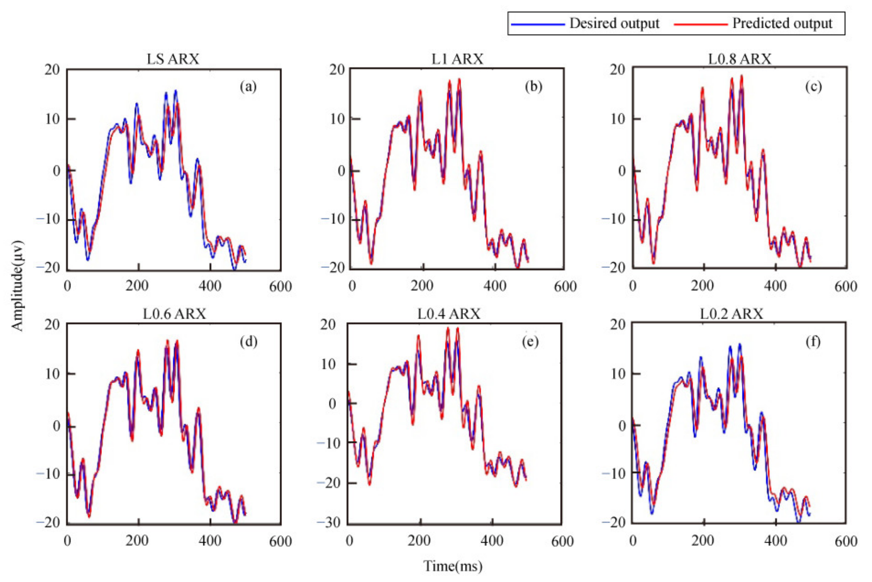
3.2.1. Application to Actual EEG Recordings

The above simulation study reveals that outliers have obvious influences on ARX parameter estimation. In EEG recordings, ocular artifacts are inevitable, and they will unexpectedly disturb the signal analysis. Based on the similar results for various Lp-ARX models revealed in the simulation study and the relatively high efficiency of L1-ARX implementation, in this section, we concentrated on the different performances between L1-ARX and LS-ARX in the SISO system when they were applied to resting-state EEG datasets that are contaminated with ocular artifacts.

The details of this dataset can be found in [32]. This study was carried out in accordance with the recommendations of the Ethics Committee of the University of Electronic Science and Technology of China. For each subject, we visually selected one 1.5 s EEG segment with obvious ocular artifacts from the whole recording for performance evaluation. For the real data study, we selected the EEG at Fp1 as the system input and the EEG at Fpz as the system output. For both signals, the first 1 s data with obvious ocular artifacts were utilized to estimate the model parameters. The remaining part of the output signal was regarded as the ground truth. We predicted the system output by substituting the remaining system input and the estimated model’s parameters into Equation (1). We calculated the predicting errors between the predicted output and the ground truth to evaluate the performance of L1-ARX and LS-ARX on system identification under the influence of ocular artifacts. Two typical waveforms of both the input and output signals are illustrated in Figure 3.

Figure 4 depicts the fitting performance for the two methods, where the red curve is the ground truth, the green curve depicts the output predicted by L1-ARX and the blue curve represents the predicted output of LS-ARX. We can see intuitively that the fitting result of L1-ARX is better than that of LS-ARX. Though the results presented here are from a single subject, the results from other subjects are similar to those revealed in Figure 4. In

Table 9. The error (μv) of the predicted signal with the two ARX models.

Subject	Method
	LS-ARX	L1-ARX
1	9.2295	7.7953
2	7.3647	6.4325
3	7.3430	6.4876
4	5.0670	4.0245
5	4.3612	3.3372
6	5.5014	4.5819
7	6.8686	5.4962
8	7.5475	6.5210
9	5.3146	4.1594
10	5.6730	4.5378
11	9.7528	8.3152
Average	6.7294 ± 1.73	5.6081 ± 1.62 *

“*” indicates the significant difference (p ≤ 0.05) between LS-ARX and the L1-ARX model.

, we can see that the L1-ARX model is a more robust method for dealing with outliers than the LS-ARX model according to the fitting errors.

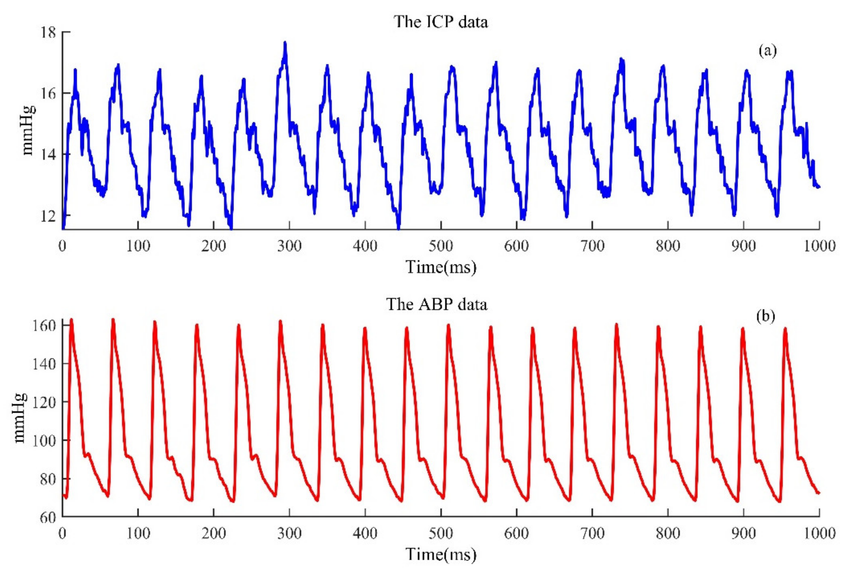
3.2.2. Application to Actual EEG Recordings

Another application for ARX in system identification was to estimate intracranial pressure (ICP) by ABP. However, both ICP and ABP are usually contaminated with artifacts, which may influence the parameter estimation of the ARX model and result in serious fitting errors. In this subsection, we utilized the dataset reported to evaluate the performance of both L1-ARX and LS-ARX. This database was recorded from 15 patients. Each patient had 5- to 25-min-long ABP and ICP recordings. The details of this dataset can be found in [5]. For each subject, we visually selected two 2 s segments from the whole recording of both the ICP and ABP for analysis. In this study, we regarded the ABP as the system input and the ICP as the system output. For both the input and output, the first segment is depicted in Figure 5 for model-parameter estimation, and Figure 6 depicts the second segment that is used for performance evaluation.

With the estimated system parameters and the second segment of the system input, we predicted the system output. The mean value of the ICP, predicting errors and correlation coefficients between the desired and the predicted system output are collected in

Table 10. The mean of the intracranial pressure (ICP) data.

Subject	Method
	LS (mmHg)	L1 (mmHg)	Real (mmHg)
1	13.7831	13.8759	14.2000
2	18.5624	18.6203	19.0778
3	8.6183	8.7711	9.3489
4	23.7407	23.8564	24.4172
5	17.1373	17.2725	17.8372
6	24.0823	24.2048	25.0012
7	19.7513	19.7813	20.8477
8	19.8864	19.9744	20.7015
9	21.5216	21.5523	21.9293
10	17.0425	17.0672	17.1580
11	14.9890	15.1406	16.3673
12	7.8933	7.9316	8.4423
13	3.9604	4.0621	4.5802
14	7.7528	7.9307	8.5877
15	9.3349	9.5021	10.0645

and

Table 11. The error (mmHg) and correlation coefficient (CC) of the predicted signal with the ARX models.

Subject	Method
	LS ARX		L1 ARX
	Error	CC	Error	CC
1	0.4482	0.9152	0.3754	0.9766
2	0.5306	0.9502	0.4794	0.9839
3	0.6162	0.8519	0.4943	0.9790
4	0.6807	0.9894	0.5715	0.9989
5	0.3293	0.9151	0.2718	0.9936
6	0.9217	0.9484	0.8011	0.9951
7	1.0964	0.9024	1.0664	0.9347
8	0.3779	0.8940	0.3384	0.9954
9	0.4364	0.9610	0.4118	0.9936
10	0.2154	0.9127	0.2069	0.9525
11	1.3784	0.9018	1.2268	0.9776
12	0.3072	0.8706	0.2888	0.9895
13	0.3116	0.8814	0.2654	0.9251
14	0.5458	0.8570	0.4354	0.9846
15	0.4512	0.9392	0.3528	0.9871
Mean Result	0.5765 ± 0.32	0.9127 ± 0.04	0.5057 ± 0.30 *	0.9778 ± 0.02 *

“*” indicates the significant difference (p ≤ 0.05) between LS-ARX and the L1-ARX model.

. “*” indicates a significant difference (p < 0.05 for all variables) between L1-ARX and LS-ARX. To intuitively compare the prediction efficiency of the two models, we show the system output waveforms in Figure 7, where the red curve is the desired system output, the green curve is the predicted output by L1-ARX, and the blue curve represents the predicted output by LS-ARX.

4. Discussion

The existence of outliers is a major challenge in biomedical signal analysis. Our simulation study based on intracranial monkey EEG quantitatively evaluates the robustness of the proposed model to outlier effects. The conducted comparison reveals that both the proposed Lp-ARX (p = 1.0, 0.8, 0.6, 0.4, 0.2) and conventional L2 norm-based ARX are influenced by outliers. Both model parameter biases and waveform fitting errors in Table 1, Table 2, Table 3 and Table 4 increase when the number of outliers increases from 8 to 24. Another aspect that needs to be noted is that the parameter bias and fitting errors in Table 3 and Table 4 are higher than those in Table 1 and Table 2, which may be caused by the lower causal relationship between the two selected system inputs. Though the parameter bias and fitting errors in Table 3 and Table 4 are higher than those in Table 1 and Table 2, the results of all Lp-ARXs (p = 1.0, 0.8, 0.6, 0.4, 0.2) are still better than those of LS-ARX. Table 5, Table 6, Table 7 and Table 8 further reveal that ARX parameter estimation is largely influenced by the strength of the outliers, i.e., stronger outliers result in more biased ARX parameters. However, for all the simulation results, the Lp-ARX (p = 1.0, 0.8, 0.6, 0.4, 0.2) models consistently show significantly better performance than LS-ARX with p < 0.05 for all conditions. Outliers with large amplitudes will be exaggerated in the objective function of the ARX model because of the square property when they are adopted for parameter estimation. Therefore, the L2 norm-based ARX focuses on fitting the outliers while other detailed information is neglected. When the ARX model is structured in Lp (p ≤ 1) norm space, the objective functions hold the ability to suppress outlier influence, as shown in previous studies [32]. Evidently, the different mathematical characteristics of the Lp norm account for different performances of the Lp-ARX models in the simulation study. In theory, smaller p (p ≤ 1) will facilitate the compress outlier effect, as shown in Table 4 and Table 8. However, when p is smaller than one, the gradient of the Lp object function involves the rooting operation, which may dramatically increase the algorithm complexity. Moreover, when p is close to zero, the estimation of the gradient becomes unstable and results in biased model parameters. In addition, to enrich the content, we also evaluated Huber loss according to the same experimental configuration. The performance of Huber-ARX is better than that of LS-ARX but weaker than that of Lp-ARX. Moreover, the variance of the results is too large, which indicates that the model is unstable.

Similar to the findings in the simulation study, the application to real EEG recordings also consistently indicates better performances of L1-ARX compared with LS-ARXs in dealing with ocular artifacts. The results in Table 9 demonstrate that a smaller fitting error can be obtained by L1-ARX than by LS-ARX, which is similar to what we discussed above.

In addition to system identification in EEG, various studies have shown that the change of ICP is tightly associated with ABP waveforms, and the estimation of ICP using ICP-related ABP by a series of system identification strategies offers a promising solution for noninvasive ICP assessment [5]. In this work, we conducted an analysis of performance evaluation for both L1-ARX and LS-ARX on ICP estimation with ABP when the data were contaminated with outliers. As shown in Table 11, the mean ICP error calculated with L1-ARX is significantly smaller than that calculated by LS-ARX. Consistent with the ICP errors, the mean ICP correlation coefficients calculated with L1-ARX are significantly higher than those calculated with LS-ARX. The coefficients modeling the relationship between ICP and ABP play a crucial role in the system output prediction. The better results for both ICP error and the correlation coefficients further indicate the robustness of L1-ARX in the application of system identification when the data are contaminated with outliers.

The conducted experiments of both real EEG data and ICP estimation with ABP illustrate the superiority of L1-ARX relative to LS-ARX in system identification when both the system input and output are contaminated with artifacts. In other words, the performance efficiency of the Lp-ARX (p ≤ 1) method is better than the conventional LS method in data fitting processing, especially when the data are affected by outliers. Moreover, we think the Lp-ARX model may also be a potential method for biomedical signal processing in other applications, such as magnetoencephalography (MEG). We will conduct more investigations to probe the usefulness of our proposed Lp-ARX in our future work.

5. Conclusions

In this work, we utilize the merits of the Lp (p ≤ 1) norm for the suppression of outliers to build a new ARX model. To verify the robustness of the proposed model, we conducted the simulation experiments and adopted it in the actual datasets. Moreover, to further verify the proposed model, we conducted the compared experiments with the conventional methods. The simulation experimental results demonstrated that the proposed method could estimate ARX parameters more robustly than conventional methods under various outlier conditions, whether for the outlier occurrence rate or the outlier strength. In the actual application, the resting-state EEG with ocular artifacts demonstrated that the proposed method could predict missing data with less influence from the artifacts, and the results on ICP and ABP data further verified its efficiency for model fitting and system identification. The proposed Lp-ARX may hold great potential in the processing of biomedical signals. Furthermore, we adopted the Lp (p ≤ 1) norm in the widely used linear dynamic model, and the non-linear model has not been explored in this work. Considering the underlying non-linear relationship in time series, in future work, we will extend the proposed Lp (p ≤ 1) method to the non-linear ARX models, which is capable of capturing the more complicated couplings among time series.

References

1. Monden, Y.; Yamada, M.; Arimoto, S. Fast Algorithm for Identification of an Arx Model and Its Order Determination. IEEE Trans. Acoust. Speech Signal Proces. 1982, 30, 390–399. [Google Scholar] [CrossRef]
2. Isaksson, A.J. Identification of Arx-Models Subject to Missing Data. IEEE Trans. Autom. Control 2002, 38, 813–819. [Google Scholar] [CrossRef]
3. Jin, G.D.; Lu, L.B.; Zhu, X.F. A Method of Order Determination for Arx and Arma Models Based on Nonnegative Garrote. Appl. Mech. Mater. 2014, 721, 496–499. [Google Scholar] [CrossRef]
4. Nelles, O. Nonlinear System Identification: From Classical Approaches to Neuralnetworks and Fuzzy Models. Appl. Ther. 2001, 6, 717–721. [Google Scholar]
5. Xu, P.; Kasprowicz, M.; Bergsneider, M.; Hu, X. Improved Noninvasive Intracranial Pressure Assessment with Nonlinear Kernel Regression. IEEE Trans. Inform. Technol. Biomed. 2010, 14, 971–978. [Google Scholar]
6. Wang, Z.; Xu, P.; Liu, T.; Tian, Y.; Lei, X.; Yao, D. Robust Removal of Ocular Artifacts by Combining Independent Component Analysis and System Identification. Biomed. Signal Proces. Control 2014, 10, 250–259. [Google Scholar] [CrossRef]
7. Nguyen, V.T.; Breakspear, M.; Cunnington, R. Fusing Concurrent Eeg–Fmri with Dynamic Causal Modeling: Application to Effective Connectivity During Face Perception. NeuroImage 2013, 102, 60–70. [Google Scholar] [CrossRef]
8. Gourévitch, B.; Kay, L.M.; Martin, C. Directional Coupling from the Olfactory Bulb to the Hippocampus During a Go/No-Go Odor Discrimination Task. J. Neurophysiol. 2010, 103, 2633–2641. [Google Scholar] [CrossRef]
9. Zhao, Y.; Billings, S.A.; Wei, H.-L.; Sarrigiannis, P.G. A Parametric Method to Measure Time-Varying Linear and Nonlinear Causality with Applications to Eeg Data. IEEE Trans. Biomed. Eng. 2013, 60, 3141–3148. [Google Scholar] [CrossRef]
10. Siuly, S.; Li, Y. Discriminating the Brain Activities for Brain–Computer Interface Applications through the Optimal Allocation-Based Approach. Neural Comput. Appl. 2015, 26, 799–811. [Google Scholar] [CrossRef]
11. Burke, D.P.; Kelly, S.P.; De Chazal, P.; Reilly, R.B.; Finucane, C. A Parametric Feature Extraction and Classification Strategy for Brain-Computer Interfacing. IEEE Trans. Neural Syst. Rehabil. Eng. 2005, 13, 12–17. [Google Scholar] [CrossRef] [PubMed] [Green Version]
12. Li, Y.; Wei, H.-L.; Billings, S.A.; Sarrigiannis, P. Time-Varying Model Identification for Time–Frequency Feature Extraction from Eeg Data. J. Neurosci. Meth. 2011, 196, 151–158. [Google Scholar] [CrossRef] [PubMed] [Green Version]
13. Qidwai, U.; Shakir, M.; Malik, A.S.; Kamel, N. Parametric Modeling of Eeg Signals with Real Patient Data for Simulating Seizures and Pre-Seizures. In Proceedings of the 2013 International Conference on Human Computer Interactions, Chennai, India, 23–24 August 2013; pp. 1–5. [Google Scholar]
14. Yu, H.; Guo, X.; Qin, Q.; Deng, Y.; Wang, J.; Liu, J.; Cao, Y. Synchrony Dynamics Underlying Effective Connectivity Reconstruction of Neuronal Circuits. Phys. Stat. Mech. Appl. 2017, 471, 674–687. [Google Scholar] [CrossRef]
15. Yu, H.; Wu, X.; Cai, L.; Deng, B.; Wang, J. Modulation of Spectral Power and Functional Connectivity in Human Brain by Acupuncture Stimulation. IEEE Trans. Neural Syst. Rehabil. Eng. 2018, 26, 977–986. [Google Scholar] [CrossRef]
16. Liao, W.; Mantini, D.; Zhang, Z.; Pan, Z.; Ding, J.; Gong, Q.; Yang, Y.; Chen, H. Evaluating the Effective Connectivity of Resting State Networks Using Conditional Granger Causality. Biol. Cybern. 2010, 102, 57–69. [Google Scholar] [CrossRef] [PubMed]
17. Kim, S.; Putrino, D.; Ghosh, S.; Brown, E.N. A Granger Causality Measure for Point Process Models of Ensemble Neural Spiking Activity. PLoS Comput. Biol. 2011, 7, e1001110. [Google Scholar] [CrossRef] [PubMed] [Green Version]
18. Kwak, N. Principal Component Analysis Based on L1-Norm Maximization. IEEE Trans. Pattern Anal. Mach. Intell. 2008, 30, 1672–1680. [Google Scholar] [CrossRef]
19. Xu, P.; Tian, Y.; Chen, H.; Yao, D. Lp Norm Iterative Sparse Solution for Eeg Source Localization. IEEE Trans. Biomed. Eng. 2007, 54, 400–409. [Google Scholar] [CrossRef] [PubMed]
20. Li, P.; Xu, P.; Zhang, R.; Guo, L.; Yao, D. L1 Norm Based Common Spatial Patterns Decomposition for Scalp Eeg Bci. Biomed. Eng. Online 2013, 12, 77. [Google Scholar] [CrossRef] [Green Version]
21. Mattsson, P.; Zachariah, D.; Stoica, P. Recursive Identification Method for Piecewise Arx Models: A Sparse Estimation Approach. IEEE Trans. Signal Proces. 2016, 64, 5082–5093. [Google Scholar] [CrossRef]
22. Guo, S.; Wang, Z.; Ruan, Q. Enhancing Sparsity Via ℓp (0<P<1) Minimization for Robust Face Recognition. Neurocomputing 2013, 99, 592–602. [Google Scholar]
23. Chartrand, R.; Staneva, V. Restricted Isometry Properties and Nonconvex Compressive Sensing. Inverse Probl. 2008, 24, 035020. [Google Scholar] [CrossRef] [Green Version]
24. Chartrand, R. Exact Reconstruction of Sparse Signals Via Nonconvex Minimization. IEEE Signal Process. Lett. 2007, 14, 707–710. [Google Scholar] [CrossRef]
25. Foucart, S.; Lai, M.-J. Sparsest Solutions of Underdetermined Linear Systems Via ℓq-Minimization for 0 <Q ⩽ 1. Comput. Harmon. Anal. 2009, 26, 395–407. [Google Scholar]
26. Nie, F.; Huang, Y.; Wang, X.; Huang, H. New Primal Svm Solver with Linear Computational Cost for Big Data Classifications. In Proceedings of the 31st International Conference on International Conference on Machine Learning, Beijing, China, 22–24 June 2014; Volume 32, pp. II-505–II-513. [Google Scholar]
27. Ye, Q.; Fu, L.; Zhang, Z.; Zhao, H.; Naiem, M. Lp-and Ls-Norm Distance Based Robust Linear Discriminant Analysis. Neural Netw. 2018, 105, 393–404. [Google Scholar] [CrossRef]
28. Wang, H.; Nie, F.; Cai, W.; Huang, H. Semi-Supervised Robust Dictionary Learning Via Efficient L-Norms Minimization. In Proceedings of the IEEE International Conference on Computer Vision, Sydney, Australia, 1–8 December 2013; pp. 1145–1152. [Google Scholar]
29. Lustig, M.; Donoho, D.; Pauly, J.M. Sparse Mri: The Application of Compressed Sensing for Rapid Mr Imaging. Magn. Reson. Med. 2007, 58, 1182–1195. [Google Scholar] [CrossRef]
30. Chartrand, R. Fast Algorithms for Nonconvex Compressive Sensing: Mri Reconstruction from Very Few Data. In Proceedings of the 2009 IEEE International Symposium on Biomedical Imaging: From Nano to Macro, Boston, MA, USA, 28 June–1 July 2009; pp. 262–265. [Google Scholar]
31. Li, P.; Wang, X.; Li, F.; Zhang, R.; Ma, T.; Peng, Y.; Lei, X.; Tian, Y.; Guo, D.; Liu, T. Autoregressive Model in the Lp Norm Space for Eeg Analysis. J. Neurosci. Methods 2015, 240, 170–178. [Google Scholar] [CrossRef] [PubMed]
32. Li, P.; Huang, X.; Li, F.; Wang, X.; Zhou, W.; Liu, H.; Ma, T.; Zhang, T.; Guo, D.; Yao, D. Robust Granger Analysis in Lp Norm Space for Directed Eeg Network Analysis. IEEE Trans. Neural Syst. Rehabil. Eng. 2017, 25, 1959–1969. [Google Scholar] [CrossRef] [PubMed]
33. Rahim, M.A.; Ramasamy, M.; Tufa, L.D.; Faisal, A. Iterative Closed-Loop Identification of Mimo Systems Using Arx-Based Leaky Least Mean Square Algorithm. In Proceedings of the 2014 IEEE International Conference on Control System, Computing and Engineering, Penang, Malaysia, 28–30 November 2014; pp. 611–616. [Google Scholar]
34. Broyden, C.G. Quasi-Newton Methods and Their Application to Function Minimisation. Math. Comput. 1993, 21, 368–381. [Google Scholar] [CrossRef]
35. Pavon, M. A Variational Derivation of a Class of Bfgs-Like Methods. Optimization 2018, 67, 2081–2089. [Google Scholar] [CrossRef] [Green Version]
36. Goldfarb, D. A Family of Variable-Metric Methods Derived by Variational Means. Math. Comput. 1970, 24, 23–26. [Google Scholar] [CrossRef]
37. Fletcher, R. A New Variational Result for Quasi-Newton Formulae. SIAM J. Optim. 1991, 1, 18–21. [Google Scholar] [CrossRef]
38. Shanno, D.F. Conditioning of Quasi-Newton Methods for Function Minimization. Math. Comput. 1970, 24, 647–656. [Google Scholar] [CrossRef]
39. Broyden, C.G. A Class of Methods for Solving Nonlinear Simultaneous Equations. Math. Comput. 1965, 19, 577–593. [Google Scholar] [CrossRef]
40. Robitaille, B.; Marcos, B.; Veillette, M.; Payre, G. Quasi-Newton Methods for Training Neural Networks. WIT Trans. Inform. Commun. Technol. 1993, 2. [Google Scholar] [CrossRef]
41. Broyden, C.G. The Convergence of a Class of Double-Rank Minimization Algorithms 1. General Considerations. IMA J. Appl. Math. 1970, 6, 76–90. [Google Scholar] [CrossRef]
42. Nagasaka, Y.; Shimoda, K.; Fujii, N. Multidimensional Recording (Mdr) and Data Sharing: An Ecological Open Research and Educational Platform for Neuroscience. PLoS ONE 2011, 6, e22561. [Google Scholar] [CrossRef] [Green Version]
43. Hardin, J.W. Generalized Estimating Equations (Gee); John Wiley & Sons, Ltd.: Hoboken, NJ, USA, 2005. [Google Scholar]
44. Wu, H.; Sun, D.; Zhou, Z. Model Identification of a Micro Air Vehicle in Loitering Flight Based on Attitude Performance Evaluation. IEEE Trans. Robot. 2004, 20, 702–712. [Google Scholar] [CrossRef]
Figure 1. The output and input waveforms mingled with outliers. (a) The system input. (b) The system output.
Electronics 10 00755 g001
Figure 2. The waveforms of the desired output and the predicted results from six ARXs when outliers were mixed in the original data. (a) The predictive performance of the LS-ARX model. (bf) The predictive performance of the Lp-ARX model (p = 1, 0.8, 0.6, 0.4, 0.2).
Electronics 10 00755 g002
Figure 3. The input and output waveforms. (a) The system input. (b) The system output. The time series on the left side of the green dotted line is used for parameter estimation, and the data on the right side indicate the fitting results of both ARX models.
Electronics 10 00755 g003
Figure 4. The predicted results of the model. The red curve is the desired system output, the green curve is the predicted output by L1-ARX, and the blue curve represents the output predicted by LS-ARX. For the convenience of display, we only draw the prediction results for a certain period of time.
Electronics 10 00755 g004
Figure 5. The system output and system input for parameter estimation. (a) The original output waveform with outlier influence. (b) The original input waveform with outlier influence.
Electronics 10 00755 g005
Figure 6. The system output and system input for performance evaluation. (a) The waveform of the second system output segment. (b) The waveform of the second system input segment.
Electronics 10 00755 g006
Figure 7. The system output waveforms. The waveform depicted by the red curve is the desired system output, the blue curve depicts the predicted results by LS-ARX, and the green curve depicts the predicted results by L1-ARX. For the convenience of display, we only draw the prediction results for a certain period of time.
Electronics 10 00755 g007