An Estimation Method of an Electrical Equivalent Circuit Considering Acoustic Radiation Efficiency for a Multiple Resonant Transducer

Abstract

The electrical equivalent model of an underwater acoustic transducer must be exactly defined in the operating frequency band to improve the driving efficiency between a sonar transmitter and a transducer. This paper used the PSO (particle swarm optimization) algorithm to estimate electrical equivalent circuit parameters of a transducer that has multiple resonant modes. The proposed method used a new fitness function to minimize the estimation error between the measured impedance of the transducer and the estimated impedance. The difference to the previous method is that the proposed method considered interference effects of the adjacent resonant modes. Additionally, this paper analyzed the effective power and separated the mechanical and acoustical resistance by considering the acoustic radiation efficiency of the transducer. As a result, the proposed method estimated all parameters at the resonance points which are influenced by the adjacent resonant modes.

1. Introduction

Existing acoustic transducers used in active sonar systems have been developed for broadband, high power, and high efficiency [1,2,3,4,5]. For driving transducers in broadband, multiple resonant modes should be adjacently located in the operating frequency [4,5]. For efficiently driving transducers at a high power level, it is necessary to design an impedance matching circuit between the sonar transmitter and the transducer [1,2].

Impedance characteristics of the transducer are dependent on a variety of reasons such as transducer type, array structure, size, etc. [2,4,6]. That is why the impedance matching techniques should be considered with an equivalent circuit model for each transducer application [7,8]. An equivalent circuit model has an important role to express the physical operation phenomenon of a transducer [1,9]. An equivalent circuit model has been expressed from various topologies depending on transducer material properties or its applications [4,5].

The equivalent circuit model started with the Mason’s piezoelectric transducer 1-D model in 1942 [9,10,11]. In this model, the physical motion of a piezo ceramic is compared to a spring and is shown in an electrical circuit model by using an ideal transformer to separate an electric and a mechanical-acoustical part. In 1961, Redwood presented the circuit model with electrical transmission lines to express the transient phenomenon of the transducer operation, such as signal delay times and reflections by impedance matching [10,12]. In 1970, the KLM model was proposed for transducers operated in a high-frequency band [10,11,13,14]. The model is 2-D, which is considered the front and back acoustic parts of a ceramic, unlike the Mason model. It is still widely used in Ultrasonics, as it is a model able to show the vibration thickness mode. In 1994, Leach proposed a new model to replace the Mason model using a transformer [10]. The model includes the piezoelectric ceramic, matching, backing layer, and cable in a high-frequency band. BVD (Butterworth–Van Dyke) model is the simplest model for the simulation of a multilayer structure, but it is not suitable for high-frequency performance [10]. Despite those limitations, BVD has been preferred because of its high accuracy at the resonance point. Sherrit estimated the parameters of the equivalent circuit considering the thickness-mode vibrator [15]. M. J. Hagmann described the difference between Sherrit and BVD and proposed an advanced Sherrit model including the loss of the piezoelectric transducer which can be used in wideband [16]. The equivalent circuit model of the transducer has been studied for a long time, and findings show the base model to use will depend on its application or simplification [10,17].

The equivalent circuit model divides physical parts of the transducer; electrical, mechanical, and acoustical, which are defined by geometry, material properties, and mode constant [17]. Here, the consumption power of resistance in an acoustic part is the radiation power of the transducer. The method of increasing the radiation power is to maximize the electrical input power or to reduce mechanical loss. The matching circuit is required between the transducer and the transmitter to deliver maximum power to the transducer [18]. The transducer has complex impedance depending on the frequency band. To efficiently drive the transmitter in the operating frequency, the impedance matching circuit based on the equivalent circuit model should be designed [19]. In other words, the transmitter design is important for maximizing an acoustic source level of the Sonar system, because it is directly related to high power and high-efficiency transmitting [20,21]. For this reason, the electrical equivalent circuit, which can express well the transducer, is very helpful to design the transmitter, and it has become important for representing the actual transducer mechanism as closely as possible.

The existing analytic method to estimate parameters of an equivalent circuit is based on the approximation at each mode [10,17], but it is not exact at low effective resonant modes. The approximated method has calculated parameters of an equivalent circuit by using measured impedance and each resonant frequency of a transducer that has multiple resonant modes. However, the results were not exact to estimate the parameters of the equivalent model [22]. R. Ramesh regarded multiple resonant modes as a simple connection of every single resonant mode without the coupled effects of each mode and then used nonlinear regression and least-squares method that have two resonant modes [15]. The method increases the estimation errors in the condition that are low effective resonant modes affected by other adjacent resonant modes. The estimated values at the low effective resonant mode could mostly be missed. To determine the unknown parameters of the equivalent model, particle swarm optimization (PSO) is used to minimize the fitness function value [23]. X. peng et al presented a method to minimize the estimation errors caused by the interference effect of adjacent resonant modes and to estimate the equivalent model parameters of a relatively low effective resonant mode of the transducer [24].

This paper used the multiple resonant circuit based on the BVD model for the piezoelectric ceramic transducer. The equivalent circuit has branches due to separating mechanical and acoustical resistance at each resonant mode, in contrast to existing studies. First, Previous methods 1 and 2 find the parameters by using the PSO algorithm with the least square method. Previous method 1 estimates the circuit parameters in a way to minimize the impedance estimation errors of the transducer in the frequency band. Previous method 2 extracted resonance frequency points from the measured impedance data, and then the points made would be referred to as estimate parameters. However, the previous methods have trouble estimating the parameters at each branch when the adjacent resonant mode effect is very influential. Thus, this paper proposed a new method that has a new fitness function to exclude the mutual interference effect of each resonant mode, to isolate adjacent resonant mode. Additionally, the acoustic radiation term was separated from the total resistance of the equivalent circuit model by considering the efficiency of the transducer, based on the assumed electrical–acoustical conversion efficiency at each resonant mode.

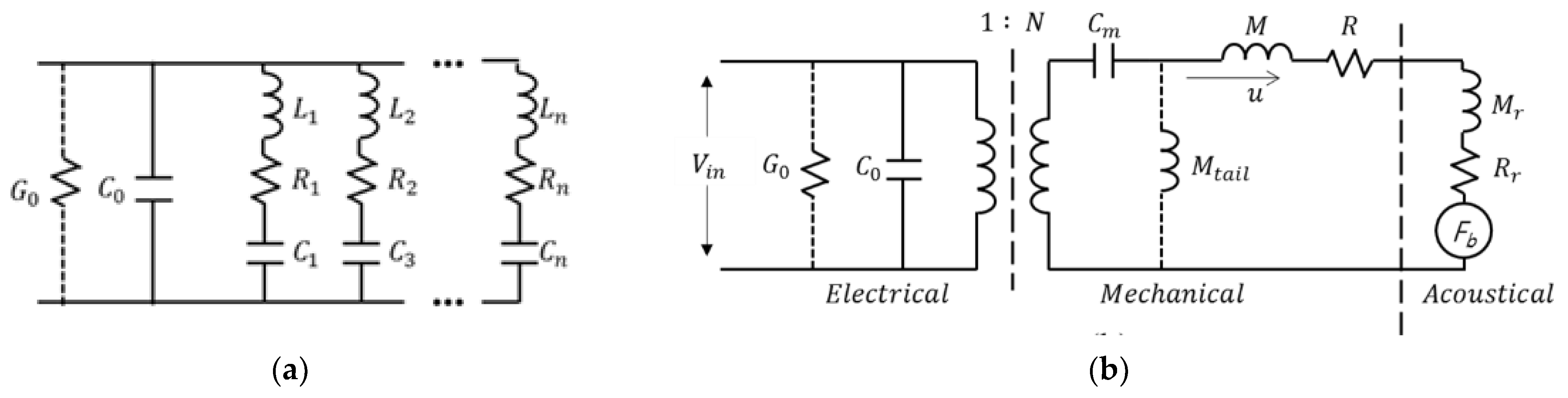
2. Equivalent Circuit Model for the Transducer

2.1. Basic Circuit Model

The BVD model having nth modes is shown in Figure 1a. This model consisted of the capacitance, C₀, and series R_n-L_n-C_n which is the element combining the mechanical and acoustical terms [15,16]. Figure 1b shows each separated section: the electrical, mechanical, and acoustical terms [25]. The loss of the acoustic radiation resistance, R_r, is the real-radiated energy of the transducer, and the resistance, R, is the mechanical loss. Large radiation resistance increases acoustic radiation energy and source level. The ratio of two resistances is defined by the transducer efficiency and is calculated by Equations (1) and (2).

$$W_e=\frac{1}{2}{G}_0{V}_{in}{}^2, W_m=\frac{1}{2}\left(R+R_r\right)u^2, W_a=\frac{1}{2}{R}_r{u}^2$$

(1)

$${\eta }_{em}=\frac{W_m}{W_e}=\frac{\left(R+R_r\right)u^2}{G_0{V}_{in}{}^2}, {\eta }_{ma}=\frac{W_a}{W_m}=\frac{R_r}{R+R_r}, {\eta }_{ea}={\eta }_{em}{\eta }_{ma}\approx \frac{R_r}{R+R_r}$$

(2)

The energies in each section, electrical (W_e), mechanical (W_m), acoustical (W_a), mean the energy loss of the circuit [25]. η_em, η_ma, η_ea are each conversion efficiency between electrical–mechanical, mechanical–acoustical, electrical–acoustical, respectively. If G₀ is assumed to be very small (large resistance), the loss at each resonance is dependent on mechanical and acoustic radiation resistance. Thus, the efficiency of each resonant mode can be approximated by using mechanical and acoustic radiation resistance [26]. From the electrical–mechanical conversion efficiency, the source level is defined as Equation (3), [21].

$$SL=170.8+10lo{g}_{10}{P}_e+10lo{g}_{10}{\eta }_{ea}+DI$$

(3)

The power P_e is the input power of the transducer. Thus, increasing input power affects the source level. The acoustic radiation energy that affects the source level can be calculated by separating R and R_r. The acoustic radiation resistance is related to the radiation area and medium of a transducer. There are two methods to find the ratio between the two resistors; one is calculated from the measured impedance of a transducer in both air and water [26], another is from the side of transducer design parameters [27]. Here, separating M and M_r was not considered because they do not significantly affect the calculation of the acoustic radiation efficiency.

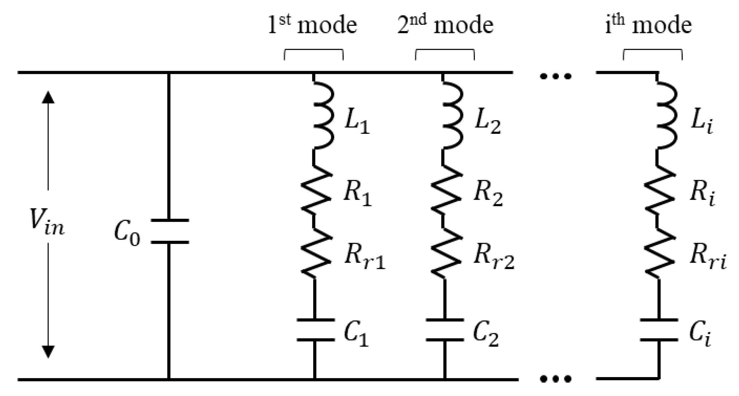
2.2. Proposed Equivalent Circuit

Figure 2 shows the electrical equivalent circuit separated by mechanical and acoustical resistance. Each resonance point in the interesting frequency band is expressed as a branch, ith mode. Each element would be estimated from the measured impedance data. Here, R_i is the mechanical resistance, R_ri is the acoustic radiation resistance. Comparing Figure 1b, the conductance, G₀ is for the small electrical loss, which can be ignored because of a reciprocal of large resistance. C_m is the stiffness, and it is displaced to C_i. M_tail is the tail mass for fixing a transducer. The tail mass has approximately two to four times heavier than the head mass [25]. For this reason, this paper ignored its effectiveness.

2.3. Transducer Model for Experiment

We measured the impedance data of a piezoelectric tonpilz transducer to verify multiple resonant modes in the interesting frequency band. The transducer was composed of cylindrical piezoelectric ceramics connected in parallel, with the head and the tail masses combined using tension bolts. The acoustic window was attached to the head mass of the transducer and the components of the transducer were enclosed in water-tight housing.

We measured the impedance magnitude and phase of the transducer in the water tank by an impedance analyzer (4194A, HP) at intervals of 100 Hz. From the measured impedance data, each frequency point that corresponds to the peak impedance (conductance) values would be the resonant point. The frequency band at each resonant mode could be identified by using the minimum point of the conductance.

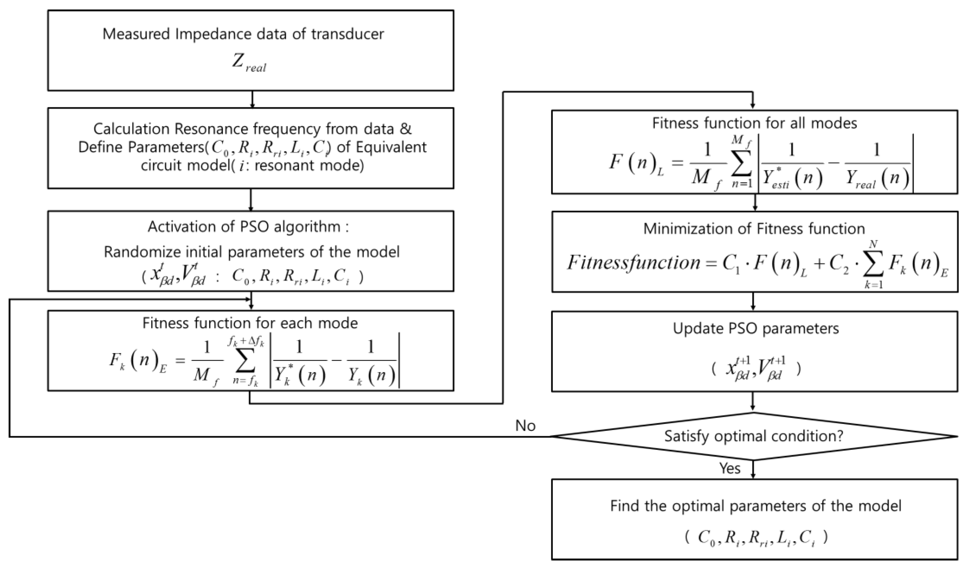
3. Estimation of Equivalent Circuit Model

This paper used the PSO Algorithm to determine the unknown parameters because the algorithm can quickly find multiple parameters without a complicated boundary condition. The equation is in Equations (4) and (5) and the parameter explanation is shown in

Table 1. The parameters for Equations (4) and (5).

Symbol	Description
$w_1$,$w_2$	Acceleration constants (usually set 2)
$d$	Number of swarm (1, 2, …, D)
$D$	Total number of unknown parameters of the equivalent model
$r_1$,$r_2$	Uniformly distributed random numbers (between 0 and 2)
$\gamma$	Inertia weight factor
$\delta$	Number of particles (1, 2, …, b)
b	Total number of particles for the swarm (unknown parameters of the equivalent model)
$V_{\delta d}^t$	Present velocity vector of the individual particle
$V_{\delta d}^{t+1}$	Next velocity vector of the individual particle
$x_{\delta d}^t$	Present position vector of the individual particle
$x_{\delta d}^{t+1}$	Next position vector of the individual particle
$gbes{t}_d$	Best position vector of the swarm
$pbes{t}_{\delta d}$	Best position vector of the individual particle

.

$$V_{\delta d}^{t+1}=\gamma ·V_{\beta d}^t+w_1{r}_1\times \left(pbes{t}_{\delta d}-x_{\beta d}^t\right)+w_2{r}_2\times \left(gbes{t}_d-x_{\delta d}^t\right)$$

(4)

$$x_{\delta d}^{t+1}=x_{\delta d}^t+V_{\delta d}^{t+1}$$

(5)

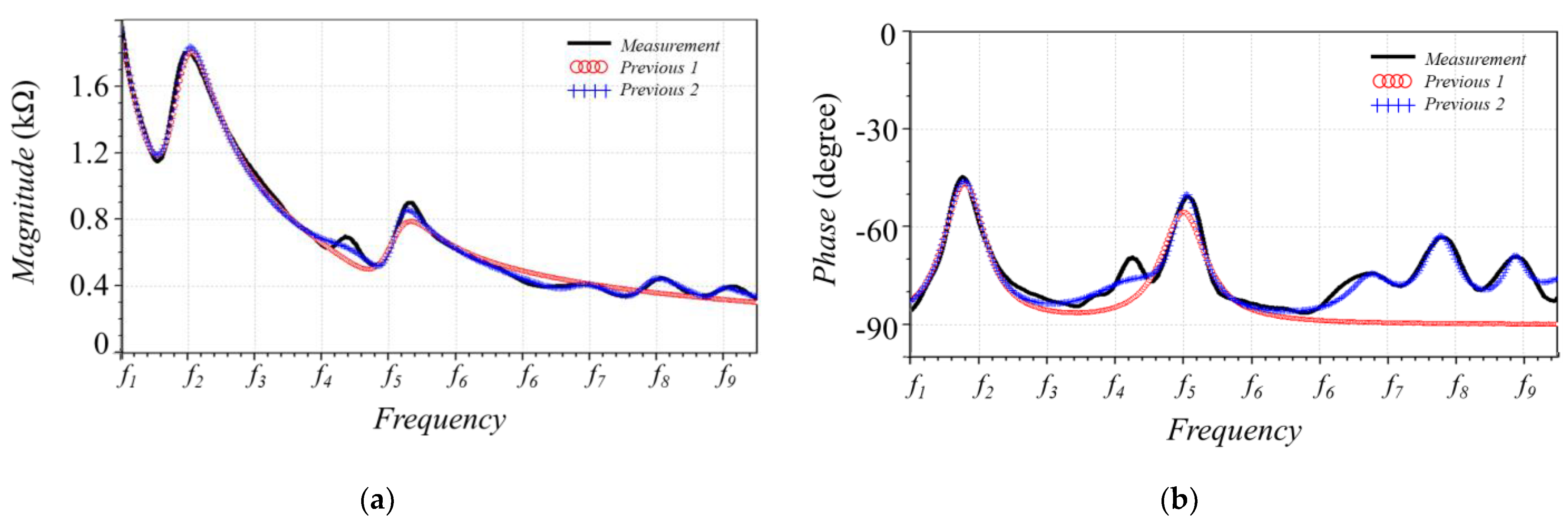
3.1. Previous Method

3.1.1. Previous Fitness Function

Previous method 1 only used the least square method to minimize the estimation error between the estimated impedance, Z*_esti(n), and the measured impedance, Z_real(n). The PSO algorithm estimates the parameters of the equivalent circuit through iteration minimizing the error of each real and complex impedance term. The fitness function is expressed in (6), (7), and parameter explanation is shown in

Table 2. The parameters for Equations (6) and (7).

Symbol	Description
n	Data sample for the frequency band
Mf	Number of the total data sample of the measured impedance
Z*esti(n)	Estimated impedance of the equivalent circuit model for nth data sample
Zreal(n)	Measured impedance of the transducer for nth data sample
α(n)	Impedance real term of the transducer for nth data sample
β(n)	Impedance imaginary term of the transducer for nth data sample

.

$$Z_{esti}^{*}\left(n\right)={\alpha }^{*}\left(n\right)+j{\beta }^{*}\left(n\right), Z_{real}=\alpha \left(n\right)+j\beta \left(n\right)$$

(6)

$$F{\left(n\right)}_L=\frac{1}{M_f}{\displaystyle \sum }_{n=1}^{M_f}\left|Z^{*}{}_{esti}\left(n\right)-Z_{real}\left(n\right)\right|=\frac{1}{M_f}{\displaystyle \sum }_{n=1}^{M_f}\sqrt{{\left({\alpha }^{*}\left(n\right)-\alpha \left(n\right)\right)}^2+{\left({\beta }^{*}\left(n\right)-\beta \left(n\right)\right)}^2}$$

(7)

Its disadvantage cannot exactly estimate the multiple resonant modes because overall estimation error would be dependent on the biggest resonance point. For this reason, Previous method 1 is used to estimate only a single resonance point. Previous method 2 estimates parameters after finding each resonance point. This method improves the convergence speed by reducing the number of parameters because either L_i or C_i is decided by the resonance point. Another method is to find all resonance points, and then give a different weight factor at each point. However, it is not used in this paper, because multiple weight factors can interfere to minimize estimation errors.

3.1.2. Results

Figure 3 shows the impedance magnitude and phase of an underwater acoustic transducer having multiple resonant modes in the interesting frequency band. The estimated impedance data by using Previous methods 1 and 2 are compared with the measured impedance magnitude and phase. The results of Previous method 1 only estimated high effective resonance points, the first and third, because of minimizing the estimated error focused on overall data. The results of Previous method 2 seems to estimate the data better in the vicinity of resonant modes than Previous method 1, due to finding resonance points before estimation. However, the Previous method 2 missed the second resonant mode because the two adjacent modes of the second mode affected the estimation error of the second mode. The estimation results show that only using the least square method is limited in minimizing the estimation error.

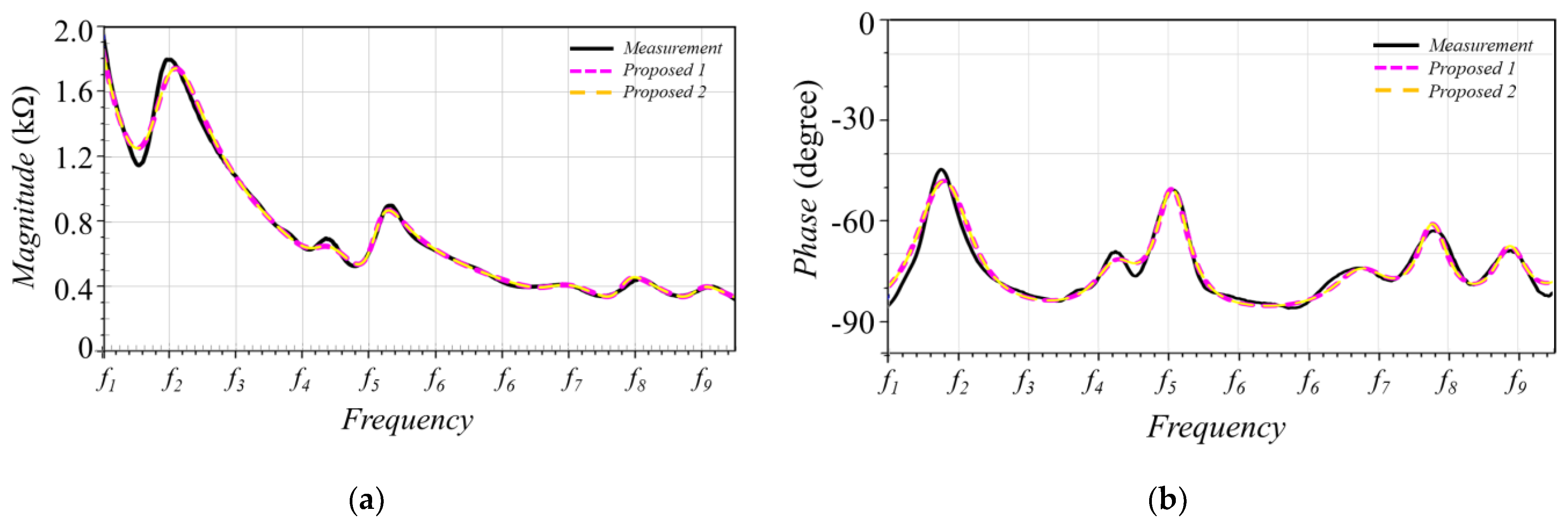
3.2. Proposed Method

3.2.1. Proposed Fitness Function

The Proposed method added the term minimizing estimation errors at each resonant mode on the Previous method. F_all is the part to minimize the estimation error by using the least square method between the measured and estimated impedance which was described in the Previous method. F_k is the part to minimize the estimation error at each resonant mode. The revised fitness function is expressed in Equations (8)–(11), and parameter explanation is shown in

Table 3. The parameters for the Equations (8)–(11).

Symbol	Description
$f_k$	Starting frequency (data sample) of kth resonant mode
$\Delta f_{k }$	Frequency band of kth mode
$Y_{esti}^{*}\left(n\right)$	Estimated admittance of the equivalent circuit model for nth data sample
$Y_{real}\left(n\right)$	Measured admittance of the transducer for nth data sample
$Y_k^{*}\left(n\right)$	Estimated admittance of the kth branch for nth data sample
$Y_k\left(n\right)$	Measured admittance of the kth resonant mode for nth data sample
$Y_i\left(n\right)$	Estimated admittance of the ith ($i\ne k)$ branch for nth data sample

.

$$F{\left(n\right)}_p=c_1·F{\left(n\right)}_L+c_2·{\displaystyle \sum }_{k=1}^N{F}_k{\left(n\right)}_E$$

(8)

$$F{\left(n\right)}_L=\frac{1}{M_f}·{\displaystyle \sum }_{n=1}^{M_f}\left|\frac{1}{Y_{esti}^{*}\left(n\right)}-\frac{1}{Y_{real}\left(n\right)}\right|,F_k{\left(n\right)}_E=\frac{1}{M_f}·{\displaystyle \sum }_{M=f_k}^{f_k+\Delta f_k}\left|\frac{1}{Y_k^{*}\left(n\right)}-\frac{1}{Y_k\left(n\right)}\right|$$

(9)

$$Y_k^{*}\left(n\right)=Y_{real}\left(n\right)-\left(Y_0\left(n\right)+{\displaystyle \sum }_{\begin{array}{c}i=1\\ i\ne k\end{array}}^N{Y}_i\left(n\right)\right)$$

(10)

$$Y_0\left(n\right)=j\omega C_0,Y_i\left(n\right)=\frac{1}{\left(R_i+R_{ri}\right)+j\omega L_i+\frac{1}{j\omega c_i}}$$

(11)

The revised fitness function cannot reduce the estimation errors but eliminates the influence of other adjacent resonant modes at each branch. Here, a branch represents one of the resonant modes. The weight factors, c₁ and c₂, are applied to the fundamental fitness function (F_L) and added function (F_k), respectively. They are usually defined through simulation experience or by the transducer impedance characteristics. Selecting weight factors of the fitness function is one of the important things to decide an estimation method, because the weight factors affect the convergence speed, the number of iteration, or the desired results. This paper decided c₁ = 2, c₂ = 1.

Figure 4 shows the estimation algorithm of the equivalent circuit model. First, the impedance data of a transducer should be measured in an experiment. From the impedance data, resonant frequency points and frequency sections divided by each branch are respectively calculated. The parameters ($C_o, R_i, R_{ri}, L_i, C_i)$ of the equivalent circuit model are randomly selected as initial values. In each resonance mode, the fitness function firstly performs the elimination of the influence of the other adjacent resonant modes. In all resonance modes, the fitness function minimizes errors between measurement and estimation. The optimized parameters will be estimated by using the PSO algorithm to minimize the estimated errors through fitness function, as described by Equations (8)–(11).

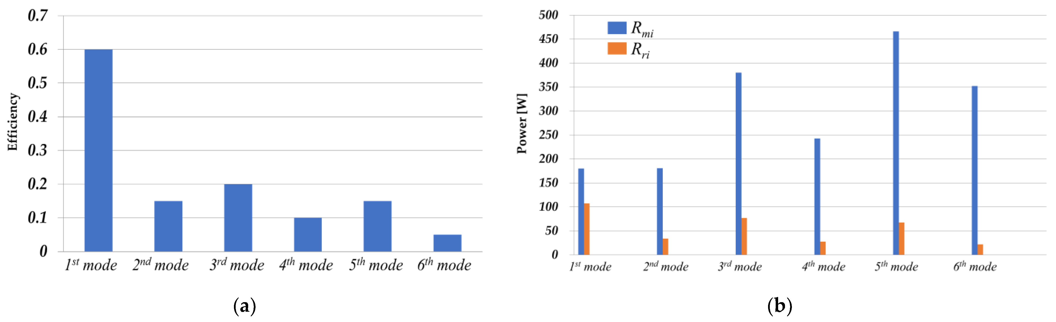
3.2.2. Separated Mechanical and Acoustic Radiation Resistance

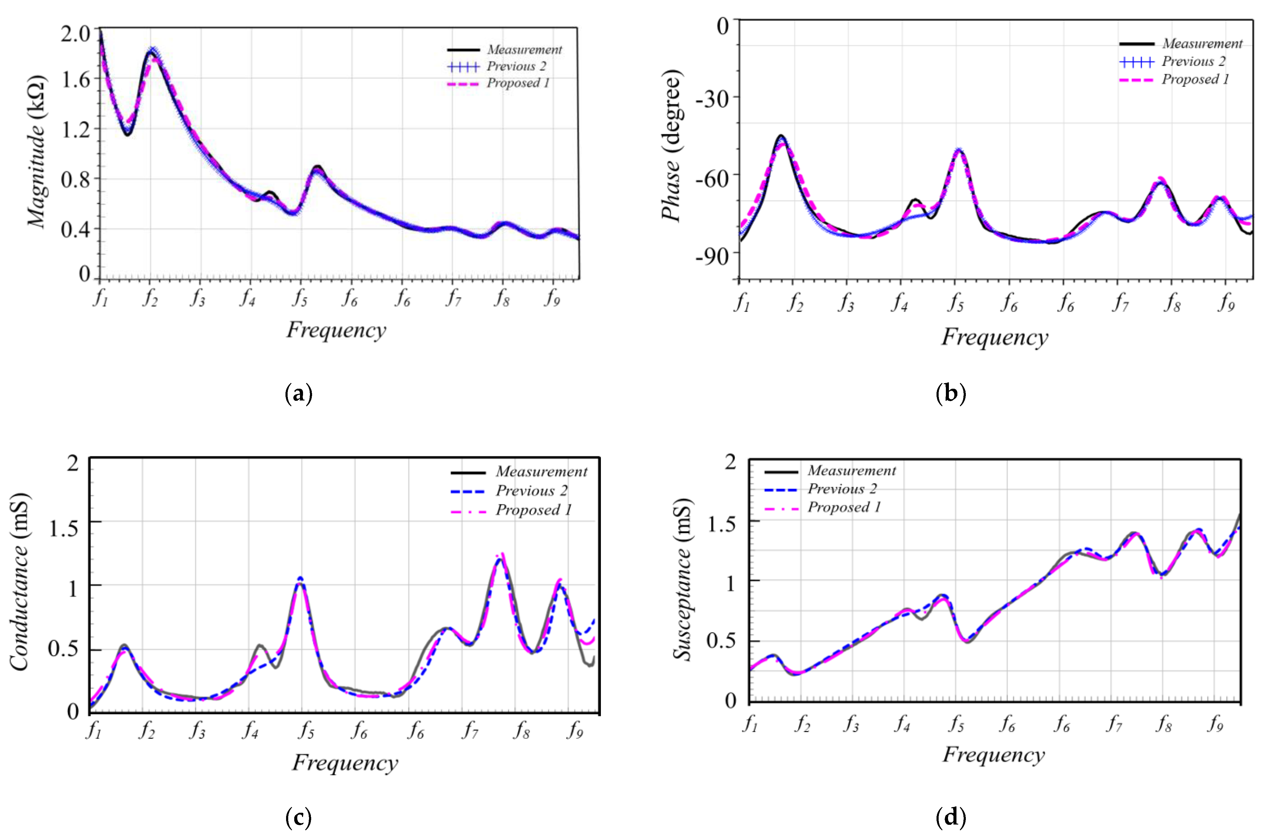
When designing a sonar transmitter, the output voltage and power are calculated to satisfy a required acoustic source level of arrayed transducers. In the general process, the electrical equivalent circuit is firstly estimated from the measured impedance of the transducer, and then, the output voltage and power of the transmitter for driving the transducer are determined. Through the assumed driving efficiency of the transducer, this paper proposed the circuit model separated mechanical and acoustic radiation resistance, to predict the acoustic source level. The ratio of two resistances at each resonant mode is defined by the mechanical and acoustical term of the transducer, as expressed in Equation (12)

$${\eta }_i=\frac{R_{ri}}{R_{mi}}=\frac{R_{ri}}{R_{ri}+R_i}$$

(12)

The mechanical resistance is R_i, and the radiation resistance is R_ri. The sum of the resistance is R_mi. η_i is an electrical–acoustical conversion efficiency divided by the resistors for ith resonant mode. This paper assumed the conversion efficiency by referring to general piezo-transducers, their efficiencies are less than approximately 70%. [22,23]. Equation (13) and (14) show admittances substituting the efficiency, η_i, into the revised fitness function as described in Equation (10) and (11).

$$Y_i\left(n\right)=\frac{\left(1/\left(1-{\eta }_i\right)\right)R_i-j\left(\omega L_i-1/\omega C_i\right)}{{\left(1/\left(1-{\eta }_i\right)\right)}^2{R}_i{}^2+{\left(\omega L_i-1/\omega C_i\right)}^2}$$

(13)

$$Y_k^{*}\left(n\right)=Y_{real}\left(n\right)-{\displaystyle \sum }_{\begin{array}{c}i=1\\ i\ne k\end{array}}^N\frac{\left(1/\left(1-{\eta }_i\right)\right)R_i}{{\left(1/\left(1-{\eta }_i\right)\right)}^2{R}_i{}^2+{\left(\omega L_i-1/\omega C_i\right)}^2}+j\left(\omega C_0-{\displaystyle \sum }_{\begin{array}{c}i=1\\ i\ne k\end{array}}^N\frac{\omega L_i-1/\omega C_i}{{\left(1/\left(1-{\eta }_i\right)\right)}^2{R}_i{}^2+{\left(\omega L_i-1/\omega C_i\right)}^2}\right)$$

(14)

3.2.3. Results

For accurately estimating the equivalent circuit’s parameters at each branch, Proposed method 1 excluded the impedance effects of other modes to estimate one mode. It was intended to exclude interference among the other resonant modes. The estimated results are shown in Figure 5. More details, conductance, and susceptance are shown in Figure 5c,d. All resonance points, including a low effective resonant mode, are estimated better than Previous method 2. Especially, the second resonant mode was fitted to the measured data. Figure 6 shows the results of Proposed method 2 which is the estimation method using the equivalent circuit model with the separated mechanical–acoustical resistance. The results should be similar to Proposed method 1 because the resistors were separated considering the electrical–acoustical conversion efficiency. Considering the adjacent resonant mode (second mode), the first mode is slightly off the measured data, but it is small.

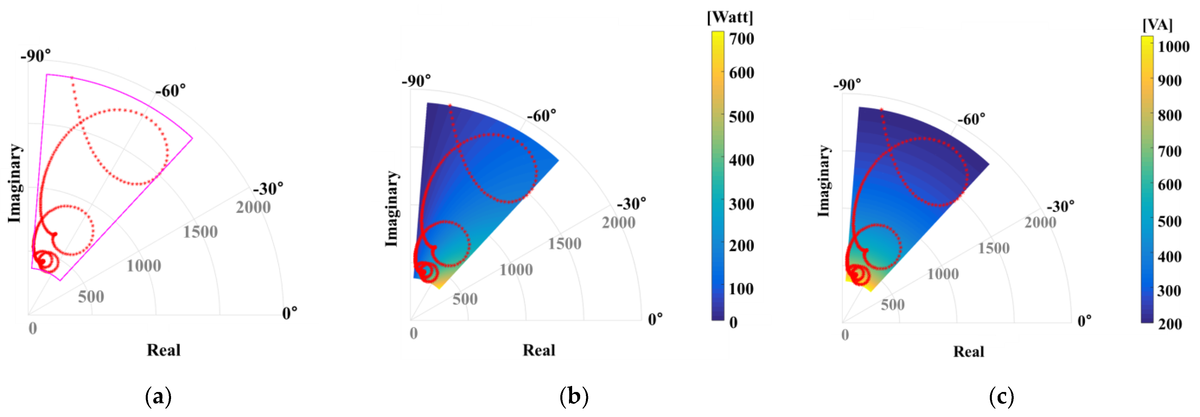
3.3. Effective Power

3.3.1. Simulation Condition

For calculating the effective power at each mode, the transmitter is driven as the output voltage, approximately 610 [V_rms] considering the rated power (the impedance is approximately 1200 [Ω] and −50° at the first resonant frequency). The effective power of the equivalent circuit model is expressed in Equations (15) and (16). P_Rmi is the effective power for the sum of the mechanical and acoustic radiation resistances. P_Rri is the real acoustic radiation power of the transducer. The estimated parameters of the equivalent circuit model at each resonant mode are shown in

Table 4. The estimated parameters in each mode.

Parameter			Previous 1	Previous 2	Proposed 1	Proposed 2
	C0	[nF]	13.0	11.0	10.9	10.9
1st mode	Rr1	[Ω]	-	-	-	1257.2
	R1	[Ω]	0.0	1978.2	2095.4	838.1
	L1	[mH]	7900.2	116.0	93.0	93.0
	C1	[nF]	10.5	4.9	6.1	6.1
2nd mode	Rr2	[Ω]	-	-	-	424.2
	R2	[Ω]	1048.0	3757.0	2828.0	2403.8
	L2	[mH]	54.7	105.7	153.0	153.0
	C2	[nF]	1.2	0.8	0.6	0.6
3rd mode	Rr3	[Ω]	-	-	-	220.7
	R3	[Ω]	120.4	1115.7	1103.3	882.7
	L3	[mH]	11401.2	90.2	81.8	81.8
	C3	[nF]	60.2	0.7	0.8	0.8
4th mode	Rr4	[Ω]	-	-	-	182.3
	R4	[Ω]	6023.3	1914.6	1822.6	1640.3
	L4	[mH]	180,356.8	96.4	72.4	72.4
	C4	[nF]	0.4	0.3	0.4	0.4
5th mode	Rr5	[Ω]	-	-	-	104.7
	R5	[Ω]	41.0	973.9	937.7	797.0
	L5	[mH]	12,487.3	61.3	70.3	70.3
	C5	[nF]	19.7	0.3	0.3	0.3
6th mode	Rr6	[Ω]	-	-	-	60.1
	R6	[Ω]	1972.5	1488.8	1202.3	1142.2
	L6	[mH]	110.9	141.2	85.4	85.4
	C6	[nF]	5.1	0.1	0.2	0.2

.

$$P_{Rmi}={\displaystyle \sum }_{i=1}^N\left|V_{norm}^2\times \frac{R_i+R_{ri}}{{\left(R_i+R_{ri}+j\omega L_i+{\frac{1}{j\omega C}}_i\right)}^2}\right|$$

(15)

$$P_{Rri}={\displaystyle \sum }_{i=1}^N\left|V_{norm}^2\times \frac{R_{ri}}{{\left(R_i+R_{ri}+j\omega L_i+{\frac{1}{j\omega C}}_i\right)}^2}\right|$$

(16)

3.3.2. Results

Figure 7a shows the complex impedance of the equivalent circuit model indicated in the polar coordination system. The X-axis and Y-axis are the real and imaginary terms, respectively. The boundary line means the impedance distribution estimated in the equivalent circuit model of the transducer. The red dot is the impedance magnitude and phase of the equivalent circuit model in the interest frequency band. Figure 7b shows the effective and apparent power for driving the transducer. The effective power for driving the transducer is distributed in the range from 179.9 to 465.8 [W]. In the area, the apparent power is in the range from 197.6~1020.6 [VA]. Thus, the value excluding the effective power from apparent power becomes the reactive power. To reduce the unnecessary reactive power, an impedance matching of the transducer should be applied in resonant modes.

For analyzing the acoustic radiation power, the electrical–acoustical conversion efficiency at each resonant mode is assumed, as shown in Figure 8a. The total effective power and acoustic radiation power are described in Figure 8b. Each power can be expressed as the loss of total resistance, R_mi, and the acoustic radiation power of the resistance, R_ri, when driving each mode of the transducer. The acoustic radiation power increasing the source level is not proportional to total effective power, because of the electrical–acoustical efficiency. In the third and fifth modes, the acoustic radiation powers are similar to the first resonant mode, but the mechanical losses are higher than the first resonant mode. For the acoustic operation, a large amount of power is required in those modes.

4. Conclusions

This paper studied methods of estimating the parameters in the equivalent circuit model from the measured impedance data of a transducer. The previous methods cannot estimate a low effective resonant mode by the interference of the adjacent resonant mode because of using the general fitness function. This paper proposed a new fitness function to exclude the interference of other modes in the vicinity of each mode. As a result, all resonant modes, including interference of adjacent resonant modes, were relatively well-estimated. The proposed method is expected to design the sonar transmitter driving broadband transducers.

By estimating the parameters of the equivalent circuit model to consider electrical–acoustical conversion efficiency, the acoustic radiation resistance can be separated from the total resistance for each resonant mode. The conversion efficiency was assumed for analyzing acoustic radiation power at each mode. Through the equivalent circuit model of the transducer, a sonar transmitter including matching and filter circuits can be designed to improve the power efficiency and power factor. In a sonar system, analyzing the effective power is expected to identify the transducer modes that can be driven by the transmitter.

5. Patents

No. US 10408927B2.

References

1. Choi, J.H.; Mok, H.S. Simultaneous Design of Low-Pass Filter with Impedance Matching Transformer for SONAR Transducer Using Particle Swarm Optimization. Energies 2019, 12, 4646. [Google Scholar] [CrossRef] [Green Version]
2. Song, S.M.; Kim, I.D.; Lee, B.H.; Lee, J.M. Design of Matching Circuit Transformer for High-Power Transmitter of Active Sonar. J. Electr. Eng. Technol. 2020, 15, 2145–2155. [Google Scholar] [CrossRef]
3. Choi, J.; Lee, D.H.; Mok, H. Discontinuous PWM Techniques of Three-Leg Two-Phase Voltage Source Inverter for Sonar System. IEEE Access 2020, 8, 199864–199881. [Google Scholar] [CrossRef]
4. Butler, J.L.; Butler, A.L. Ultra wideband multiple resonant transducer. IEEE Ocean. 2003, 5, 2381–2387. [Google Scholar]
5. Edalafar, F.; Azimi, S.; Qureshi, A.Q.A.; Yaghootkar, B.; Keast, A.; Friedrich, B.B. A wideband, low-noise accelerometer for sonar wave detection. IEEE Sens. 2017, 18, 508–516. [Google Scholar] [CrossRef]
6. Chen, Z.; Zhang, Q.; Li, C.; Fu, S.; Qiu, X.; Wang, X.; Wu, H. Geometric nonlinear model for prediction of frequency–temperature behavior of SAW devices for nanosensor applications. Sensors 2020, 20, 4237. [Google Scholar] [CrossRef]
7. Kim, S.; Wang, H.; Park, I.; Lee, K. Toward real time monitoring of wafer temperature in plasma chamber through surface acoustic wave resonator and mu-negative metamaterial antenna. IEEE Sens. J. 2021, 21, 19863–19871. [Google Scholar] [CrossRef]
8. Crupi, G.; Gugliandolo, G.; Campobello, G.; Donato, N. Measurement-Based Extraction and Analysis of a Temperature-Dependent Equivalent-Circuit Model for a SAW Resonator: From Room Down to Cryogenic Temperatures. IEEE Sens. J. 2021, 21, 12202–12211. [Google Scholar]
9. Bybi, A.; Mouhat, O.; Garoum, M.; Drissi, H.; Grondel, S. One-dimensional equivalent circuit for ultrasonic transducer arrays. Appl. Acoust. 2019, 156, 246–257. [Google Scholar] [CrossRef]
10. Shen, Z.; Xu, J.; Li, Z.; Chen, Y.; Cui, Y.; Jian, X. An Improved Equivalent Circuit Simulation of High Frequency Ultrasound Transducer. Front. Mater. 2021, 8, 109. [Google Scholar] [CrossRef]
11. Oakley, C.G. Calculation of ultrasonic transducer signal-to-noise ratios using the KLM model. IEEE Trans. Ultrason. Ferroelectr. Freq. Control 1997, 44, 1018–1026. [Google Scholar] [CrossRef]
12. Redwood, M. Transient performance of a piezoelectric transducer. J. Acoust. Soc. Am. 1961, 33, 527–536. [Google Scholar] [CrossRef]
13. Sherrit, S.; Mukherjee, B.K. Characterization of piezoelectric materials for transducers. arXiv 2007, arXiv:0711.2657. [Google Scholar]
14. Galliere, J.M.; Latorre, L.; Papet, P. A 2-D KLM model for disk-shape piezoelectric transducers. In Proceedings of the 2009 Second International Conference on Advances in Circuits, Electronics and Micro-Electronics, Sliema, Malta, 11–16 October 2009; pp. 40–43. [Google Scholar]
15. Ramesh, R.; Ebenezer, D.D. Equivalent Circuit for Broadband Underwater Transducer. IEEE Trans. Ultrason. Ferroelectr. Freq. Control 2008, 55, 2079–2083. [Google Scholar] [CrossRef]
16. Hagmann, M.J. Analysis and equivalent circuit for accurate wideband calculations of the impedance for a piezoelectric transducer having loss. AIP Adv. 2019, 9, 085313. [Google Scholar] [CrossRef]
17. Smyth, K.; Kim, S.G. Experiment and simulation validated analytical equivalent circuit model for piezoelectric micromachined ultrasonic transducers. IEEE Trans. Ultrason. Ferroelectr. Freq. Control 2015, 62, 744–765. [Google Scholar] [CrossRef] [PubMed] [Green Version]
18. Rathod, V.T. A review of electric impedance matching techniques for piezoelectric sensors, actuators and transducers. Electronics 2019, 8, 169. [Google Scholar] [CrossRef] [Green Version]
19. Yang, C.; Sun, H.; Liu, S.; Qiu, L.; Fang, Z.; Zheng, Y. A Broadband Resonant Noise Matching Technique for Piezoelectric Ultrasound Transducers. IEEE Sens. J. 2019, 20, 4290–4299. [Google Scholar] [CrossRef]
20. Lu, S.; Boussaid, F. An inductorless self-controlled rectifier for piezoelectric energy harvesting. Sensors 2015, 15, 29192–29208. [Google Scholar] [CrossRef] [Green Version]
21. Bereketli, A.; Bilgen, S. Remotely powered underwater acoustic sensor networks. IEEE Sens. J. 2012, 12, 3467–3472. [Google Scholar] [CrossRef]
22. Coates, D.; Maguire, P.T. Multiple-Mode Acoustic Transducer Calculations. IEEE Trans. Ultrason. Ferroelectr. Freq. Control 1989, 36, 471–473. [Google Scholar] [CrossRef] [PubMed]
23. Chen, D.; Zhao, J.; Fei, C.; Li, D.; Zhu, Y.; Li, Z.; Guo, R.; Lou, L.; Feng, W.; Yang, Y. Particle Swarm Optimization Algorithm-Based Design Method for Ultrasonic Transducers. Micromachines 2020, 11, 715. [Google Scholar] [CrossRef] [PubMed]
24. Peng, X.; Hu, L.; Liu, W.; Fu, X. Model-Based Analysis and Regulating Approach of Air-Coupled Transducers with Spurious Resonance. Sensors 2020, 20, 6184. [Google Scholar] [CrossRef] [PubMed]
25. Sherman, C.H.; Butler, J.L. Transducers and Arrays for Underwater Sound; Springer: SBerlin/Heidelberg, Germany, 2007; pp. 58–75. [Google Scholar]
26. Hwang, Y.H.; Ahn, H.M.; Nguyen, D.N.; Kim, W.H.; Moon, W.K. An underwater parametric array source transducer composed of PZT/thin-polymer composite. Sens. Actuators 2018, 279, 601–616. [Google Scholar] [CrossRef]
27. Kim, J.W.; Roh, Y.R. Modeling and Design of a Rear-Mounted Underwater Projector Using Equivalent Circuits. Sensors 2020, 20, 7085. [Google Scholar] [CrossRef]
Figure 1. The electrical equivalent circuit for the transducer; (a) Butterworth–Van Dyke model for multiple resonant modes, (b) Mason model for single resonant mode.
Electronics 10 02416 g001
Figure 2. The electrical equivalent circuit separated by mechanical and acoustical radiation resistance.
Electronics 10 02416 g002
Figure 3. The impedance magnitude and phase graphs for comparing previous methods and the measured data: (a) The impedance magnitude data in the frequency band; (b) The phase data in the frequency band.
Electronics 10 02416 g003
Figure 4. The algorithm block diagram of the proposed estimation method.
Electronics 10 02416 g004
Figure 5. The impedance magnitude and phase, and admittance graphs for comparing the previous method 2, proposed method and the measured data: (a) The impedance magnitude data in the frequency band; (b) The phase data in the frequency band; (c) The conductance magnitude in the frequency band; (d) The susceptance magnitude in the frequency band.
Electronics 10 02416 g005
Figure 6. The impedance magnitude and phase graphs for the separated mechanical–acoustical resistance: (a) The impedance magnitude data in the frequency band; (b) The phase data in the frequency band.
Electronics 10 02416 g006
Figure 7. The effective power and the apparent power drawn in the impedance boundary: (a) the impedance variation of the equivalent circuit model, (b) the effective power of the transducer; (c) the apparent power of the transducer.
Electronics 10 02416 g007
Figure 8. The efficiency and the effective power at each resonant mode: (a) the assumed electrical–acoustical conversion efficiency; (b) the effective power calculated from the efficiency.
Electronics 10 02416 g008