A Velocity Estimation Technique for a Monocular Camera Using mmWave FMCW Radars

Abstract

Perception in terms of object detection, classification, and dynamic estimation (position and velocity) are fundamental functionalities that autonomous agents (unmanned ground vehicles, unmanned aerial vehicles, or robots) have to navigate safely and autonomously. To date, various sensors have been used individually or in combination to achieve this goal. In this paper, we present a novel method for leveraging millimeter wave radar’s (mmW radar’s) ability to accurately measure position and velocity in order to improve and optimize velocity estimation using a monocular camera (using optical flow) and machine learning techniques. The proposed method eliminates ambiguity in optical flow velocity estimation when the object of interest is at the edge of the frame or far away from the camera without requiring camera–radar calibration. Moreover, algorithms of various complexity were implemented using custom dataset, and each of them successfully detected the object and estimated its velocity accurately and independently of the object’s distance and location in frame. Here, we present a complete implementation of camera–mmW radar late feature fusion to improve the camera’s velocity estimation performance. It includes setup design, data acquisition, dataset development, and finally, implementing a lightweight ML model that successfully maps the mmW radar features to the camera, allowing it to perceive and estimate the dynamics of a target object without any calibration.

1. Introduction

Autonomous vehicles require data about the environment to make decisions for safer navigation. They use scene perception to estimate and predict the positions, velocities, and nature of objects, and their relationships with each other. For this purpose, different sensors, such as cameras, radar, lidar, and ultrasound are used individually to extract the relevant features from a scene [1]. This process is generally known as simultaneous localization and mapping (SLAM). The goal is to have the scene/environment represented in a format which could be fed into an end to end deep learning solution capable of estimating future actions. Naturally, a better representation with more data will serve the deep learning models best and improve their decision making accuracy.

A lidar system gives a 3D representation of a scene in the form of point clouds, but they are expensive, bulky, and have a large form factor [2,3]. Further, the presentation of the point clouds is not well suited for human perception, as a human cannot decipher obstacles or commonplace objects from it very reliably. It is difficult to analyze the data and the key points that the machine bases its decisions on. In addition, extracting the velocities and real-time poses of the targets computationally is very intensive, which can cause significant latency. A camera, on the other hand, gives better visual representations of most scenes, due to the latest advancements in object detection and classification, along with its fusion with lidar [4,5]. Many efforts have been made to acquire environment data without the use of lidars and radars. The methods in [6,7] used stereo cameras and proper calibration to estimate the distance of a target object. Using a monocular (single) camera, approaches based on optical flow have been used to estimate the velocity of a target object [8]. Recently, millimeter wave radar (mmW radar) has been considered one of the suitable candidates for capturing the dynamics of an object in terms of speed, longitudinal distance, and direction of travel [1]. However, they have limited fields of view (FOV), which limits their utility for perception.

Autonomous cars generally have multiple cameras to get a full 360 degree view of the surroundings. Interspersed with them are range detecting devices, such as radar and lidar. Some work has already been done to use cameras for range and velocity finding. For example, ref. [9] is one of the earliest examples of camera calibration. Reference [10] went on to show robust calibration for a multi-camera rig. Additionally, Several approaches based on camera–radar fusion are used for perception and estimating the dynamics of objects [11,12]. However, they require calibration, and slight changes in some of the parameters of either of them will cause the system to fail to work. This is not suitable for the case where the parameters have to be tuned and/or the spatial location of either camera or radar detector has to be changed. Autonomous vehicles, or drones, are moving equipment with constantly changing lighting and environment. Existing methodologies do not work with monocular cameras, as they require environmental details to correlate their pixel velocities with real world velocities.

To mitigate the above problems, in this paper, we present a novel method using camera–radar setup to map the object’s velocity measured by narrow FOV mmw radar to optimize and enhance the velocity estimated by wide FOV monocular camera employing various machine learning (ML) techniques. We exploit individual sensors’ strengths, i.e., a camera’s wide FOV (as compared to radar’s narrow FOV) and radar’s accurate velocity measurement (compared to a camera’s not accurate estimation of velocity at the edge of frame or at the larger distances using optical flow) to fuse them in such a way that a single monocular camera can detect an object and estimate the velocity accurately, thereby increasing its performance, which otherwise would not have been possible. Further, we also introduce a dataset of live traffic videos captured using a monocular camera labeled with mmW radar. The novelties of our work are listed below.

• Our system maps the position and velocity measured by mmW radar to optimize and enhance the velocity measured by a monocular camera using optical flow and various ML techniques. This serves two purposes. Firstly, the mmW radar measurement together with a ML model enhances the measurement from the camera (using optical flow). Secondly, the enhanced function of converting optical flow values to speed permits one to generalize over other objects not detected by radar.
• The proposed method does not require camera–radar calibration as in [13,14], making the setup ad hoc, simple, reliable, and adaptive.
• The ML model used here is lightweight, and eliminates the need for depth estimation, as in [8], to estimate the velocity.

We first discuss the related work in the field. We show the different approaches taken to solve the problem and present the problem statement. We then describe the dataset and how we created it. Then we give three machine learning based algorithms with increasing complexity that satisfy the hypothesis.

This article is organized into the following sections{

• Section 2. Related Work: Discussion on the related and existing work in the field.
• Section 3. Solution Approaches: Elucidating the approaches taken for solving the problem statement.

  –

  Section 3.1. Dataset Description: We show how we generated a dataset for the problem statement.

  –

  Section 3.2. Dataset Format: We describe the format of the dataset for the purpose of reuse.

  –

  Section 3.3. Post-Processing: We describe the post-processing applied to the raw captured dataset.

  –

  Section 3.4. Hypothesis: We show a simple working model to motivate more complex solutions.

  –

  Section 3.5. Convolutional network: We show a working model with a simple convolutional neural network.

  –

  Section 3.6. Regression: We show that it is possible to predict speeds using linear regression.

  –

  Section 3.7. Yolo (You Only Look Once): We combine the convolution and regression methods into a single method to finally give a model capable of predicting bounding boxes and speeds.

• Section 4. Results and Discussion: We summarize the results from our different models and compare them with the related work.
• Section 5. Conclusion: We conclude the article and provide some future research areas.

2. Related Work

There is much work done in this field using a combination of radar, lidar, and stereo cameras. Most commonly, stereo cameras are used, which mimic the human eye system to predict depth. Tracking objects in a depth map allows us to extract velocity information. Some solutions use the intrinsic property of cameras, which involves translation of camera coordinates to the real world. This works by transforming optical flow displacement vectors to real-world displacement vectors and then using the simple speed formula to determine the speed. Another way is to determine the geometry of the environment and use it to understand scene. For, example, [13] used the known height and angle of the camera to understand the environment and calculated speed using the distance traveled by a car. They detected the license plate’s corner points to track the car, which adds another limitation, as cars can only be tracked with the license plate in view. The implementation in [15] was very similar and suffers from the same drawbacks. Camera calibration to transform pixel displacement vectors to real world object displacement vectors has also been used by [16]. A similar method was proposed in [17], where first a camera is auto-calibrated on a road, and then a transformation, as above, is used to predict vehicle speeds. However, again, the method requires calibration based on features of roads. The approach in [18] uses optical flow, but still relies on the distance of the car from the driveway line and other road features. Reference [19] also presented a method that works along the same lines. Reference [20] presented a method that uses color calibration to detect cars and then uses the angle of a fixed camera to translate pixel velocities to real world velocities. Camera properties are can also be used for transformation based prediction, as in [14].

Similarly, some points of interest in the footage can be compared with already available maps or images to estimate displacement [21]. One study [22] involved tracking license plates from a camera with known parameters. Another [23] involved a similar method but with two cameras. Their goal was to use wide-beam radars with cameras to reduce speed prediction errors. The study presented in reference [24] used the projective transformation method to generate top-down views from CCTV cameras to predict the motion of vehicles. They used background subtraction to remove background information and only focused on the roads. The study presented in reference [25] also used background subtraction and obtained real world coordinates of the car. After comparing two frames, and knowing the real world distance and time in between frames, they could predict the speed of a car. The study presented in [26] also used a similar method. The study presented in [27] used the track lines form roads to estimate speed information. The study presented in [28] used uncalibrated cameras; however, they used known vehicle length.

However, all of these approaches need some extra information regarding the environment, intrinsic properties of a camera, or some pre-processed result.

An end-to-end deep learning system has also been suggested [8]. It uses established networks such as DepthNet [29] and FlowNet [30] to get depth estimates of the object. The features are combined and passed through a dense network to obtain velocity. Our approach differs by suggesting a much simpler feature extractor compared to the complexity of FlowNet and DepthNet. We show that it is possible to obtain velocity directly from optical flow without depth information.

The study presented in [31] used a similar approach to our approach. They predicted velocities for relative vehicles in front of a camera mounted on a moving vehicle. They used dense optical flow combined with tracking information in a long term recurrent neural network. In the end, the system output velocity and position output relative to the ego-vehicle.

We analyzed the requirements of the above methods and proposed a solution to eliminate them. Our solution involves only a single camera and removes the need for prior known information about the environment.

Radar and lidar systems are active photo emitting devices capable of estimating the depth and thus the velocity of any object they come across. While radar systems are incredibly limited in FOV, lidar systems are fairly expensive. We define the problem as, “Can we predict an object’s velocity with a single camera in real-time with little computation cost?”

We define a use case scenario for this problem as follows. A car with a radar sensor facing to its front is used to continuously feed ground truth values for objects in its FOV to train a machine learning model for a monocular camera that has a larger FOV. We can use such a system to predict speed for objects as long as a camera can see them.

3. Solution Approaches

3.1. Dataset Description

To test our hypothesis, we recorded a sequence of video captured on a busy road. The videos recorded are roughly 3 h long and provide us with many examples of prediction scenarios. Most common are cars moving in a single direction (towards and away from the camera/radar setup). We also have examples of multiple vehicles in the scene, moving in opposite directions and overlapping each other for a brief period. Adding more complexity, we have different classes of vehicles, including cars, trucks, a bus, and even motorcycles. The camera used was a PiCamera V2 at 1920 × 1080 30 FPS. The format of the videos is H264. The radar used was Texas Instrument’s 1843 mmWave Radar module. The parameters used for radar configuration are mentioned in Table 1 (see Figure 1). We attached the camera over the radar to ensure a similar center of FOV. The FOV can be seen in Figure 1B along with the radar (red board) with the camera attached on top of it connected to a Raspberry Pi 3 (Figure 1C, green board), which started camera and radar capturing synchronously. The Pi and Radar were powered by a portable power bank. A laptop was used to monitor and interact with Pi over SSH. Start times and end times were logged along with the capture rate to correlate frames from each device. We let the infrastructure record independently and used the timing and rate information to overlap them later.

Table 1. Parameters used for the 1843 mmWave Radar Module.

Parameter	Value
Operating Frequency	77 GHz
Azimuth Resolution	15 deg.
Range Resolution	0.977 m
Maximum Unambiguous Range	50 m
Maximum Radial Velocity	23.03 m/s
Radial Velocity Resolution	2.89 m/s
Frame duration	33.333 ms
Range Detection Threshold	15 dB
Doppler Detection Threshold	15 dB
SDK Version	3.2

Figure 1. Experimental setup. In clockwise order: (A) Lateral view of the setup. (B) FOV from the camera. (C) Top down view of the setup.

The devices were kept at a roughly 45 degrees angle to the road to get a greater view of the road. The FOV can be seen in the image given. Having an angle also gave us a contrast between cars near and far away from the setup. Vehicles near such an apparatus will record the same velocity on the radar as those far away but be detected multiple times as the cross-sectional areas increase. Similarly, as the area of a car per image area increases, more pixels are moving, and hence there will be a higher value of optical flow. Such contrasts are needed for the machine learning solutions to learn how to predict when a vehicle’s distance is different from what the recording apparatus assumes.

The radar was configured for the best velocity calculation with about 1.5 m² of cross-sectional area.

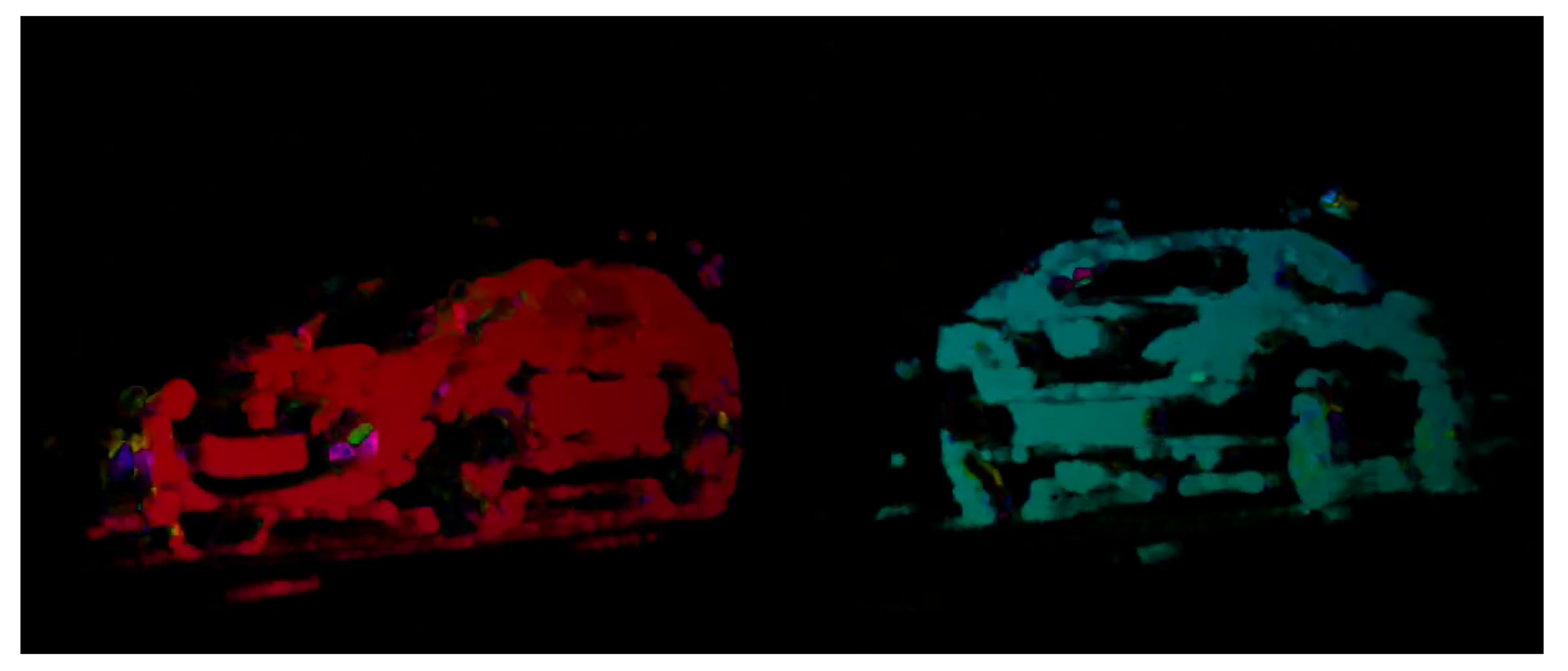
3.2. Dataset Format

The dataset is provided using TensorFlow’s TFRecord format, which stores data in Google’s protocol buffers format. Each row has a Frame ID and a Video ID to locate a frame in a particular video. They are accompanied by a raw image and an optical flow image, which are both encoded in Byte String. Raw Image is just the plain frame from the video. An optical flow image is an image generated by converting optical flow vectors into the HSV space. Specifically, the magnitude (or pixel speed) is encoded in V, and the direction in a polar form is encoded in H. This gives a result as follows, where the color indicates the direction of the car, and the intensity of the color denotes the magnitude of displacement. A sample optical flow image is shown in Figure 2. The dataset is downloadable from [32]. Table 2 can be used to create a TFRecord reader to read the dataset.

Figure 2. A sample optical flow image.

Table 2. Features of the dataset.

Feature	Description	Data Type
Frame Index	Frame order from Video	Int64
VideoId	Video Identifier	Int64
RawImage	Original Frame	Byte String
OpticalFlowImage	Optical flow of $n-1$th and nth frame	Byte String
Xmin	List of min x coordinates for BBOX	Float32 List
Xmax	List of max x coordinates for BBOX	Float32 List
Ymin	List of min y coordinates for BBOX	Float32 List
Ymax	List of max x coordinates for BBOX	Float32 List
V	List of ground truth speeds for each BBOX	Float32 List

3.3. Post-Processing

The objects in the video and radar were matched using a combination of methods. Firstly, each frame in the video and radar was timestamped. It then became a particular case of the bipartite matching problem. It should be noted that radar and camera had different frame rates. Frames from both the devices were timestamped using the recorded timing information, and frames with negligible time differences were matched. In the second step, the you only look once (YOLO) algorithm [33] was used to find bounding boxes for the cars in the FOV alongside dense optical flow using the Farneback algorithm [34]. The vehicles were either moving towards the recording apparatus or away from it, allowing for segregation of objects according to their motion directions using optical flow and radar velocities. In the third step, the segregated objects were assigned their corresponding speeds by running a k-means algorithm with the number of centroids as the number of bounding boxes. The k-means algorithm used a distance function of L2 norm between (x,y) coordinates of objects and velocities. Our dataset statistics are shown in Table 3.

Table 3. Statistics of the datasest.

Metric	Value
Sample Count	1815
Velocity range	0.00–17.50 m/s
Mean Velocities across dataset	10.80 m/s
Standard deviation of velocities across dataset	3.81

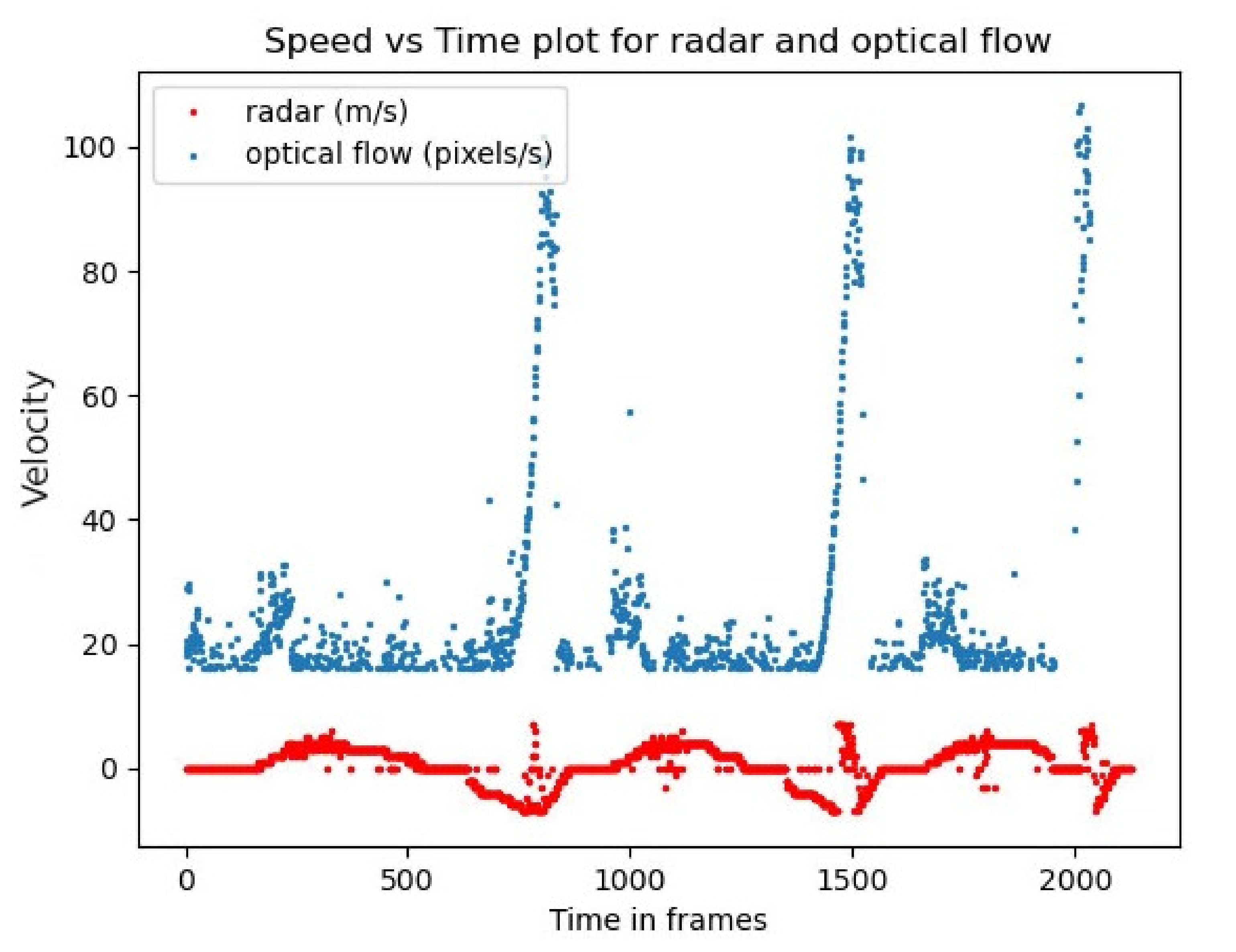
3.4. Hypothesis

To start with a simple, provable solution, we drove a car back and forth in front of the apparatus. Naturally, the reversing speeds were much lower than the other. We plotted the overlap of the optical flow with radar-measured speeds. To compare them, we used frames as time measurement unit. The optical flow speeds were calculated by taking the differences between the previous and current frames. Thus, the radar frames had to be adjusted. Recall that the radar captured at different frame rate than camera. However, with the start time and rate, we could adjust them to the same time scale. The plot is shown in Figure 3.

Figure 3. Plot of optical flow values overlapped with radar speeds against time in frames.

High peaks of optical flow depict the car’s motion towards the apparatus and the low peaks depict the reversing. It is clear that optical flow is very sensitive to car speeds, especially when the object is near to it.

3.5. Convolutional Network

Before creating a final neural network, we first created a proof of concept convolutional network. We wanted to prove that it is possible to predict the speed of a vehicle using regression alone. Additionally, we note that a car will have high optical flow values near the center of an image and low values as it moves towards the edge of an image. The reason is simple and relates to how optical flow is calculated. Optical flow measures the displacement of pixels between two frames, and given the time difference between the two frames, one could interpret these values as pixels/time. Due to the camera angle, a car will have more pixel displacement near the center of the FOV than at the edge. Therefore, we need to take into account the positions of the car and the optical flows. A convolutional network uses spatial relations and thus is best suited to this task.

We created a simple convolution model (in Figure 4) with optical flow image input in the HSV space and a single velocity output. We used HSV to visualize the optical flow images. The intensity of color represents the magnitude of optical flow per pixel, and the color itself represents the direction. We trained our model using an ADAM optimiser with early stopping after 10 epochs if the loss did not improve. Our model was trained in about 250 epochs over multiple training cycles. On Google Colab using a GPU, each training epoch took 2 s. Prediction of a frame could be performed in 0.2 ms. With a split of 80 –20, we observed convincing results with an RMSE, on average, of 2.3 across different bags of the dataset shuffled using various seeds. Our hyper-parameters for the model are mentioned in Table 4.

Figure 4. CNN architecture.

Table 4. Convolutional network hyper-parameters.

Parameter	Value
Optimizer	Adam
Optimizer Parameters	Default
Loss	rmse
Early Stopping	10 epochs
Epochs	5000
Batch Size	64
Shuffle buffer size	200

To increase the number of samples in the training dataset, each sample was augmented with random scaling, clipping, and rotation at training time. Additionally, to keep complexity in check, only the frames with single cars were considered and direction was ignored.

3.6. Regression

To further prove that regression is a viable method, we tried to approach the problem as a linear regression problem. The dataset was made table-like by converting optical flow images to HSV, as described above, and taking means across H and V channels. Averaging a cut-out of an optical flow image presents some problems, as many pixels have a value near 0. One can imagine this for a door of a car. A car door is smooth with no edges and will have no appreciable difference from pixel to pixel. Pixels in this position will be essentially 0. This characteristic is not a problem for convolutions as they use filter windows. To overcome this problem, we applied a filter and considered only pixels with appreciable values. The pixel values can vary from 0 to 255, and we repeated our experiments for different filter values, ranging from 10 to 30. Center positions of cars were calculated from a parallel YOLO object detector. The features considered were the H channel values, V channel values, center position X, and center position Y. They were regressed against the ground truth velocities for each frame. The same augmentation techniques were used for this method as well. We did not limit ourselves to a single car per frame in this scenario.

Microsoft’s open source Light Gradient Boosting Machine was used for estimation [35]. We used the parameters in Table 5 for the training.

Table 5. Regression hyper-parameters.

Metric	Value
Boosting type	Gradient Boosting Decision Tree
Test Size	0.25
Learning Rate	0.003
Max depth	50
Number of leaves	100
epochs	5000

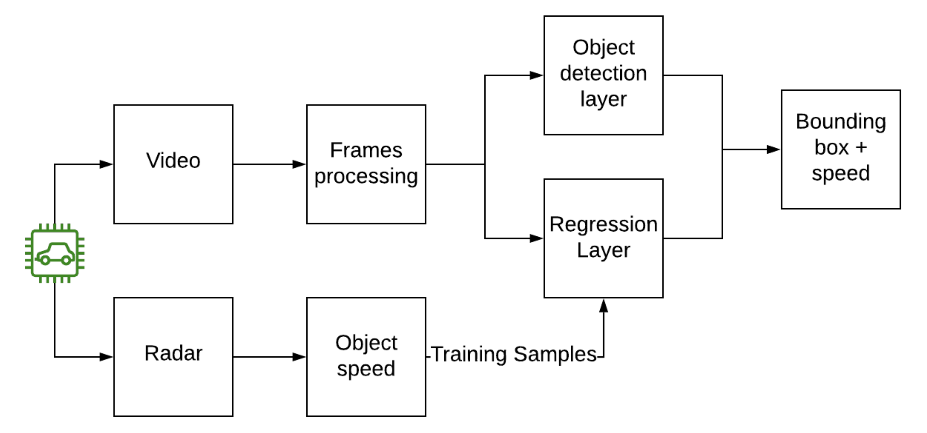
3.7. YOLO like Network

To expand upon our convolutional network POC, we took an existing network known for regression. YOLO is a very famous state-of-the-art method for object detection in images. Our arhitecture using YOLO can be seen in Figure 5. We applied the same techniques and network as YOLO with a minor change in the loss function. YOLO uses regression from end to end to detect bounding box and then uses a soft-max function to classify the boxes. We changed the soft-max to simple regression, converting the task of classification to regression. Our network simultaneously predicts the bounding box and the corresponding speed. The updated loss function is then:

Figure 5. Yolo flow diagram.

$$\begin{array}{cc}\hfill & {\lambda }_{coord}\sum _{i=0}^{S^2}\sum _{j=0}^B{1}_{ij}^{obj}[{(x_i-{\widehat{x}}_i)}^2+{(y_i-{\widehat{y}}_i)}^2]+\hfill \\ \hfill & {\lambda }_{coord}\sum _{i=0}^{S^2}\sum _{j=0}^B{1}_{ij}^{obj}[{(\sqrt{w_i}-\sqrt{{\widehat{w}}_i})}^2+{(\sqrt{h_i}-\sqrt{{\widehat{h}}_i})}^2]+\hfill \\ \hfill & {\lambda }_{obj}\sum _{i=0}^{S^2}\sum _{j=0}^B{1}_{ij}^{obj}{(C_i-{\widehat{C}}_i)}^2+{\lambda }_{noobj}\sum _{i=0}^{S^2}\sum _{j=0}^B{1}_{ij}^{obj}{(C_i-{\widehat{C}}_i)}^2+\hfill \\ \hfill & {\lambda }_{vel}\sum _{i=0}^{S^2}{1}_{ij}^{obj}\left({(V_i-{\widehat{V}}_i)}^2\right)\hfill \end{array}$$

(1)

where

$\lambda$ = scaling parameter.

$1_{ij}^{obj}=\mathrm{Indicator}\mathrm{function}\mathrm{indicating}\mathrm{that}\mathrm{an}\mathrm{object}\mathrm{exists}\mathrm{in}{i}^{\mathrm{th}}\mathrm{cell}$

$\mathrm{and}{j}^{\mathrm{th}}\mathrm{bounding}\mathrm{box}$

$x,y,w,h=\mathrm{coordinates},\mathrm{height},\mathrm{and}\mathrm{width}\mathrm{of}\mathrm{the}\mathrm{bounding}\mathrm{box}.$

There are some subtle differences from the original equation. Firstly, we have introduced new scales to prioritize different aspects of loss (values of scales and hyper-parameters are given in Table 6). Secondly, the soft-max of classes is converted to squared error. Additionally, note the absence of summation over classes for velocity, as this model can only detect one class of objects, which in this case is cars.

Table 6. YOLO network hyper-parameters.

Parameter	Value
Optimizer	Adam
Optimizer Parameters	Default
Loss	Custom
Input Image size range	288–480 (chosen randomly)
Number of Anchors	9 (3 per scale)
Non Max Suppression Threshold	0.5
${\lambda }_{coord}$	1
${\lambda }_{obj}$	2
${\lambda }_{noobj}$	1
${\lambda }_{vel}$	1
Shuffle buffer size	200

We used a pre-trained version of YOLO on the COCO dataset, taken from the author’s website, as a starting point. The model was easily trained in 30 epochs. We only report the velocity loss here for comparison and specificity.

To increase the sample size for neural networks, several data augmentation tricks were utilized. First, images were resized to an input range. Second, a random scale was selected, after which the images were stretched or cropped depending upon the size of the new scale compared to the prior. The new aspect ratio varied from 0 to a factor of 0.3 on both the axes. Thirdly, using a 0.50 probability, the images were flipped. These operations were performed simultaneously on the images and the bounding boxes to preserve the relationship.

4. Results and Discussion

Here we show a proof of concept using the convolutional network of a fast and straightforward neural network. We took this approach to the next level by using YOLO, which provided very similar results to other methods. We report only the class loss—in our case, the vehicle’s speed—as bounding box loss is irrelevant to the discussion. Our YOLO implementation had some inaccuracies in bounding box predictions, but we chalk that up to less training time and a low number of samples.

In summary, we were able to achieve error of approximately 0.93 RMSE using a YOLO-based estimator. Using a simple convolutional network and regression model, we were able to get averages of 1.93 and 2.30 RMSE, respectively. It was expected that the YOLO-based estimator would perform better, as it is more complex and has more parameters. Comparisons with other approaches are difficult, as not everyone reports their errors using the same units. Additionally, datasets used in other approaches are not readily available or do not apply to our method. Therefore, we cannot directly compare our results with other approaches, as the dataset and conditions were different for each; we still compare the loss values observed to give context to our results in Table 7. Only the directly comparative approach by [8] was fairly accurate, albeit with a big architecture taking into account a separate measurement of depth. We can see that our proposed method resulted in slightly less loss, which can be explained by the usage of different datasets. No definite conclusion can be drawn about which method works better.

Table 7. Results.

Method	Loss (RMSE)
Regression (LGBM)	1.93
Convolutional network	2.30
YOLO like network	0.93394979
Flownet + Depthnet [8]	1.12
Environment geometry using input heights [15]	0.7 percent
Environment geometry using estimated heights [15]	1.4 percent
Imaging System Geometry [13]	1.32 MAE
Using real world context [21]	0.625

Finally, we have a lightweight object detection model that works with a single camera. It can detect vehicles and classify their velocities in real-time without any calibration or environmental information. Compared to the approaches in Section 2, our approach is quite simple and straightforward to implement, without depending on any environmental or background information. Additionally, given the large FOV of camera, it is capable of detecting and classifying more objects than radar, as it only depends upon the optical flow of the object.

5. Conclusions

We presented a dataset for predicting vehicle speed, and then demonstrated the feasibility of predicting vehicle speed via a monocular camera, without the use of any environmental geometry or camera properties.

Our proposed models can be used in autonomous vehicles that are heavily dependent on vision. Cameras can help cheapen the costs of the vehicles, as they are relatively inexpensive compared to radars and lidars. The complexity is also decreased, as configuration of the cameras is not required, whereas light projecting devices do require configuration. Cameras offer advantages such as increased FOV, human understandable information, and easy setup. Hence, a fusion model such as this can be used with fewer radar detectors and more cameras to achieve same or better results in scene understanding. The ML model itself can be embedded into larger artificial intelligence models to achieve scene understanding of the car’s surroundings.

For further research, we can add the class pedestrians to the dataset. It is a challenging problem on its own because of the low walking speed of humans, the opposite motions of parts of body (such as arms swinging in the opposite directions to those of legs), and an surface area for the radar to detect. In addition, the models proposed can be implemented as part of online learning. To deal with changing lighting conditions, the models can be retrained periodically with small training samples.