Human Face Detection Techniques: A Comprehensive Review and Future Research Directions

Abstract

Face detection, which is an effortless task for humans, is complex to perform on machines. The recent veer proliferation of computational resources is paving the way for frantic advancement of face detection technology. Many astutely developed algorithms have been proposed to detect faces. However, there is little attention paid in making a comprehensive survey of the available algorithms. This paper aims at providing fourfold discussions on face detection algorithms. First, we explore a wide variety of the available face detection algorithms in five steps, including history, working procedure, advantages, limitations, and use in other fields alongside face detection. Secondly, we include a comparative evaluation among different algorithms in each single method. Thirdly, we provide detailed comparisons among the algorithms epitomized to have an all-inclusive outlook. Lastly, we conclude this study with several promising research directions to pursue. Earlier survey papers on face detection algorithms are limited to just technical details and popularly used algorithms. In our study, however, we cover detailed technical explanations of face detection algorithms and various recent sub-branches of the neural network. We present detailed comparisons among the algorithms in all-inclusive and under sub-branches. We provide the strengths and limitations of these algorithms and a novel literature survey that includes their use besides face detection.

1. Introduction

Face detection is a computer vision problem that involves finding faces in images. It is also the initial step for many face-related technologies, for instance, face verification, face modeling, head pose tracking, gender and age recognition, facial expression recognition, and many more.

Face detection is a trifling task for humans, which we can perform naturally with almost no effort. However, the task is complicated to perform via machines and requires many computationally complex steps to be undertaken. Recent developments in computational technologies have ameliorated the research in face detection. As such, many algorithms and methods for detecting faces have been proposed. Even so, there is little attention given in making a robust and updated survey of these face detection methods.

There have been some survey works referring to face detection methods. Ismail et al. [1] conducted a survey on face detection techniques in 2009. In their survey, four issues for face detection (size and types of database, illumination tolerance, facial expressions variations, and pose variations) were dealt with, along with reviews of several face detection algorithms. The algorithms reviewed were limited to principal component analysis (PCA), linear discriminant analysis (LDA), skin color, wavelet, and artificial neural network (ANN). However, a comparison between the face detection techniques was not provided for a global understanding of the methods. Omaima [2] reviewed some updated face detection methods in 2014. Focused on performance evaluation, a full comparison of several algorithms with the databases involved was presented. However, the work was only based on ANN. Among all the surveys, the survey papers by Erik and Low [3] and Ashu et al. [4] were robust and well explained. Erik and Low explained methods of face detection and the later updates on the methods quite descriptively. Ashu et al. followed the path of Erik and Low, adding face detection databases and application programming interfaces (APIs) for face detection. However, both the works are missing the recent efficient methods of face detection, such as subbranches of neural networks and statistical methods. Many recent research papers on face detection are also available in the literature [5,6,7,8,9], which, closely related to our work, attempted to review face detection algorithms. Our study, on the other hand, has conducted a more thorough review with more technical details than these reviews and is multi-dimensional as shown in

Table 1. Comparison of our work with other similar survey papers.

	Erik and Low [3]	Yang et al. [5]	Ankit et al. [6]	Ashu et al. [4]	Sarvachan et al. [7]	Mei and Deng [8]	Minaee et al. [9]	Our Work
Year	2001	2002	2017	2018	2020	2020	2021	2021
Detailed survey and discussion of different sub-areas	✓	✓	×	✓	×	×	×	✓
Branches of neural network in face detection	×	×	×	×	×	✓	✓	✓
Advantages and limitations of each algorithm	×	×	✓	✓	✓	×	×	✓
Review of a mixture of new old and recent face detection algorithm	×	✓	×	✓	×	×	×	✓
Comparison among different sub-branches	×	×	×	×	×	×	✓	✓
Implementation in other fields beside face detection	✓	×	×	×	×	×	×	✓

.

In this survey, we present a structured classification of the related literature. The literature on face detection algorithms is very diverse; therefore, structuring the relevant works in a systematic way is not a trivial task. The following are some of the contributions of this paper:

• Different face detection algorithms are reviewed in five parts, including history, working principle, advantages, limitations, and use in fields other than face detection.
• Many face detection algorithms are reviewed, such as different statistical and neural network approaches, which were neglected in the earlier literature but gained popularity recently because of hardware development.
• Systematic discrepancies are shown between algorithms for each single method.
• A comprehensive comparison between all the methods is presented.
• A list of research challenges in face detection with further research directions to pursue is given.

This paper is directed to anyone who wants to learn about the different branches of face detection algorithms. There is no perfect algorithm to use as a face detection method. However, the comparative comparisons in this paper will help to choose the algorithm to use depending on the specific problems and challenges. The description of each algorithm will aid in gaining a clear understanding of that particular process. Additionally, knowing about the history, advantages, and limitations described for each of the algorithms will assist in deciding which algorithm is best suited for any task at hand with a clear understanding.

Face detection is one of the most popular computer vision problems that involve finding faces in digital images. In recent times, face detection techniques have advanced from conventional computer vision techniques toward more sophisticated machine learning (ML) approaches. The main steps of face detection technology involve finding the area in an image where a face or faces are. The main challenges in face detection are occlusion, illuminations, and complex background. A wide variety of algorithms have been proposed to combat these challenges. Basically, the available algorithms are divided mainly on two parts: feature-based and image-based approaches. While feature-based approaches find features (image edges, corners, and other structures well localized in two dimensions), image-based approaches depend largely on image scanning, which is based on window or sub-frames.

The rest of this paper is organized as follows: In Section 2, we briefly explain the feature-based approaches as shown in Figure 1. Section 3 provides an overview of the image-based approaches. Section 4 provides a robust comparison of the face detection algorithms. Section 5 epitomizes the research challenges in face detection and further research ideas to pursue. Finally, the conclusion is presented in Section 6.

2. Feature-Based Approaches

Feature-based approaches are further divided into three sub-fields, as shown in Figure 1. The active shape models deals with complex and non-rigid shapes by deforming to fit a given example by iterative processing. In low level analysis, segmentation is performed using pixel information and is typically more concerned about individual components of a face. On the other hand, feature analysis involves organizing facial features onto a global perspective, taking into account the facial geometry.

2.1. Active Shape Model (ASM)

ASM epitomizes the actual substantial and thus, higher level appearance of features. When the system views an image, it links with facial features, such as the nose, mouth, etc., as soon as it finds a close proximity with any of these features. The coordinates of those parts are taken as a map, and from here, a mask is generated. The mask can be manually changed. Even if the system decides on the shape, this can be adjusted by the user. By training with a greater number of images, a better map can be achieved. ASMs can be classified into four groups: snakes, deformable template model (DTM), deformable part model (DPM), and point distribution model (PDM).

2.1.1. Snakes

Snakes, which are generic active contours, were first proposed by Kass et al. in 1987 [10]. Snakes are commonly utilized in locating the head boundaries [11]. To achieve the task, a snake is countersigned around the region of a head on an approximation. Once released, on the close proximity of a head, it then uses the natural evolution of snakes, which is shrinking or expanding, to gradually deform to the shape of the head. An energy function $E\left(C\right)$ matches the intuition about what makes it a good segmentation and the function [10] can be denoted as follows:

$$E\left(C\right)=E_{internal}\left(C\right)+E_{external}\left(C\right),$$

(1)

where $E_{internal}\left(C\right)$ and $E_{external}\left(C\right)$ are the internal and external energy functions, respectively. $E_{internal}\left(C\right)$ depends on the shape of the curve, while $E_{external}\left(C\right)$ depends on the image intensities (edges). The initialized snake will iteratively evolve to reduce or minimize $E\left(C\right)$.

In the minimization of the energy function, internal energy enables the snakes to shrink or expand. In contrast, external energy makes the curve fit with nearby image edges in a state of equilibrium. Elastic energy [12] is commonly used as internal energy. By contrast, external energy relies on image features. The energy minimization process requires a high computational prerequisite. This is why, for faster convergence, methods of fast iteration by greedy algorithms were employed in [13].

Snakes are autonomous and self-adapting in their search for a minimal energy state [57]. They also can be made sensitive to image scale by incorporating Gaussian smoothing in the image energy function [58]. Snakes are also relatively insensitive to noise and other ambiguities in the images because the integral operator used to find both the internal and external energy functions is an inherent noise filter. The snakes algorithm works efficiently in real-time scenarios [59]. Furthermore, snakes are easy to manipulate because the external image forces behave in an intuitive manner [60,61].

Snakes generally are capable of determining the boundaries of features but they have several limitations [62]; the contours often become trapped onto false image features, and in terms of extracting non-convex features, they are not particularly suitable [63]. The convergence criteria used in the energy minimization technique govern their accuracy; tighter convergence criteria are required for higher accuracy. This results in longer computation times. Snakes are space consuming, while the Viterbi algorithm trades space for time. This means that they require a lot of time for processing [64].

Mostafa et al. [65] used snakes algorithm to extract buildings automatically from urban aerial images. Instead of using the snakes’ traditional way of computing the weight coefficient value of the energy function, a user emphasis method was employed. A combination of genetic algorithm (GA) and snakes was used to calculate the parameters. This combination resulted in a needing fewer operators and ameliorated the speed. However, the detection accuracy was only good for detecting a single building, and it faced problems in detecting building blocks. Fang et al. presented a snake model in tracking multiple objects [66]. The model can track more than one object by splitting and connecting contours. This topology independent technique allows it to detect any number of objects unaccompanied by any exact number. Saito et al. also amalgamated GA with snakes to detect eye glass in a human face [67]. GA was used to find the parameters of snakes in this case also. The method faced problems in detecting asymmetric glasses.

2.1.2. Deformable Template Matching (DTM)

DTM model is classified as ASM because it actively deforms preset boundaries to fit a given face. Along with the face boundary, other facial features’—such as the eyes, mouth, eyebrows, nose, and ears—extraction is a pivotal task in the face detection process. The concept of snakes was taken one step further by Yuille et al. [14] in 1992 by integrating information of the eyes as a global feature for a better extraction process. The conventional template-based approach is convenient for rigid shaped faces, but suffers from problems in detecting faces with various shapes. DTM, therefore, comes with a solution by adjusting to the different shapes of the face; DTM is particularly competent with non-rigid face shapes.

DTM works by forming deformable shapes of the face, which is achieved by predefined shapes [68]. The shapes can be made in two ways: (a) polygonal templates (PT) and (b) hierarchical templates (HT). In PT, as depicted in Figure 2, a face is formed with a number of triangles, where every triangle is deformed to contort the overall version of the face [15]. On the other hand, HT functions by creating a tree shape described in Figure 3 [16].

Let us suppose that we want to find the structure of a curve from ‘a’ to ‘b’, as shown in Figure 3. A binary tree from ‘a’ to ‘b’ is built, and the process is started by selecting midpoint ‘c’. With the midpoint ‘c’, the two halves of the curve are described recursively. Other sub-nodes at the tree are made in the same way by finding the midpoints. Here, every node in the tree describes a midpoint relative to other neighboring points. Sub-trees in the tree describes sub-curves, thereby giving the local relative positions, explaining the local curvature. Adding little noise in every node, we can reconstruct the local curvature to fit any given sample recursively and thus, fit the global shape. The steepest gradient descent minimization of a combination of external energy is implicated in this deformation process.

$$E=E_v+E_e+E_p+E_i+E_{internal}.$$

(2)

Here, in Equation (2), the energy due to image brightness, valley, peak, edges, and internal energy is epitomized by $E_i$, $E_v$, $E_p$, $E_e$, and $E_{internal}$, respectively.

DTM combines local information with global information, and thus, ensures better extraction. Furthermore, it is accommodating of any type of shape in the given data [14] and can be employed in real time [69]. However, the weights of the energy terms are troublesome to interpolate. The consecutive execution of the minimization process costs an excessive processing time. To exacerbate the drawbacks, it is also sensitive to the initializing position; for instance, midpoint ‘c’ is needed to be initialized in HT.

Kluge and Lakshmanan utilized DTM in lane detection [70]. The use of DTM in detecting lanes allows likelihood of image shape (LOIS) to detect lanes without the need for thresholding and edge–non-edge classification. The detection process wholly depends on the intensity gradient information. However, the process is limited to using a smaller dataset. Jolly et al. applied DTM in vehicle segmentation [71]. A novel likelihood probability function was presented by Jolly et al. Inside and outside of the template is calculated, using directional edge-based terms. The process lacks the use of trucks, buses and trailers, like most common vehicles. Moni and Ali applied DTM, combining it with GA in object detection [72]. This combination solves the problem of optimal placement of objects in DTM. The term fitness was introduced to calculate how well random deformation fits the target shape without excessive deformation of the object. The fitness function for an object with various rotation, translation, scale or deformation was found to be harder to calculate.

2.1.3. Deformable Part Model (DPM)

DPM uses the pictorial structure for face detection, which was first proposed by Fischler and Elschlager et al. [73] in 1973. DPM is commonly employed in the detection of human faces [17,74] as well as in the detection of faces in comics [18]. DPM is a training-based model. In DPM, a face mask is formed by modeling discrete parts (eyes, nose, etc.) individually, and each of these parts are rigid parts. A set of geometric constraints are set between these parts (typically describing the distance between the eyes and nose, etc.) and can be imagined as springs, as shown in Figure 4. The intuition here is that the object parts change in appearance approximately linearly in some feature space, and the springs between these parts constrain their locations to be consistent with the deformations observed. To fit with the given data, the model is moved onto an image and stretched in different ways, trying to find a place for it that does not put too much pressure on the springs and explains that the image data are underneath the model.

The pictorial structure can be classified into two parts: part filters and root filter, as shown in Figure 4. Part filters change depending on the articulation of the face. To be particular, parts are not changing but the distance between the parts are to be incorporated with the given image.

DPM performs well in terms of detecting various shapes of faces, as it detects faces efficiently in a real-time environment [75]. Additionally, it easily detects faces with various poses and can work with variations caused by different viewpoints and illuminations [76]. However, DPM faces difficulties, such as speed bottleneck or slowness [77], and has issues in extending to new object or face categories.

Yang and Ramanan employed DPM in object detection and pose estimation [78]. The method brings forth a general framework for two things. One is the modeling of co-occurrence relations between a mixture of parts, and the other is to draw classic spatial relations, linking the positions of the parts. However, the method produces a detection problem in images with more orientation because of fewer mixture components. Yan et al. proposed a multi-pedestrian detection method, using DPM [79]. The proposed method improves the detection of pedestrian in crowded environments that have heavy occlusion. To handle occlusion, Yan et al. utilized two layer representations. On the first layer, DPM was employed to represent the part and global appearance of the pedestrians. This approach yielded a problem regarding partially visible pedestrians. The second layer was instigated by appending the subclass weights of the body. This mixture model handles various occlusions well. In an updated paper, Yan et al. [80] solved the problem of numerous resolution imaging in pedestrian detection with DPM. This updated model faced false positive results around vehicles. This particular problem was solved by constructing a context model to reduce them, depending on the pedestrian–vehicle relationship.

2.1.4. Point Distribution Model (PDM)

PDM is a shape description technique. The shape of a face is described by points in PDM. PDM was first invented by Cootes et al. [19] in 1992. However, the initial face PDM was devised by Lantis et al. [20]. PDM relies on landmark points. A landmark point is the annotation of any image onto any given shape on the training set images. The shape of a face in PDM is formed by planting landmark points on the shape of a face in the training image set. The model is generally built with a global face shape, having the formations of eyes, ears, nose, and other elements of a face, as shown in Figure 5.

In the training stage, a number of training samples are taken, where every image holds a number of points for each sample, building a shape for each. The shapes are then rigidly aligned to calculate the mean and covariance matrix. During the fitting of a PDM onto a face, the mean of the shape is positioned within reach of the face. Accordingly, a search strategy, named the gray-scale search strategy, is performed in deforming the shape to the given face. In the process, the training set controls the deformation according to the way the information is modeled within it.

PDM reduces the computation time for searching face features, as it blueprints the features while building the global face [81]. Additionally, the difficulty of occlusion of any face feature is reduced by compact global face information with features since other information of the face compensates for the occluded area [21]. PDM can be fitted with numerous face shapes and provides a compact structure of a face. However, the process of building training set by pointing out the landmarks of face and facial features is an unavoidable drudgery and, in many cases, is prone to errors. Furthermore, the control point movements are restricted to straight lines so that the line of action is linear.

Edwards et al. [82] used PDM in the human recognition, tracking and detection process. Variables, such as pose, lighting conditions and expressions, were handled up to the par. To avoid the need for a large dataset, decoupled dynamic variation models for each class were proposed, while initial approximate decoupling was allowed to be updated during a sequence. Over and above that, PDM is sometimes put to use for searching three-dimensional (3D) volume data. Comparisons among different ASM are presented in

Table 2. Comparison of different ASM.

		Active Shape Models
		Snakes [10,11,12,64]	DTM [14,15,16]	DPM [17,74,77]	PDM [19,20,21]
Similarities	Use deformation	✓	✓	✓	✓
	Need initialization point	✓	✓	✓	✓
Differences	Deformation technique	Energy minimization	PT & HT	Pictorial structure	Grey scale search strategy
	Main pitfall	Long processing time	Sensitive to initialization position	Slow	Linear processing

.

2.2. Low Level Analysis (LLA)

LLA wrenches out the descriptions of an image that are usually available in an image. LLA does not agitate with the type of object nor even the perspective of the viewer. In an image, a severe number of independent descriptors can be available, such as edges, color information, etc. For instance, if we look at an image containing a face shape, the LLA descriptors would signify where the edges of the face are, the different color variation of the face and image, etc. Provided that the descriptors are associated with an image, LLA descriptors are applicable all over the image and not just in the face structure. LLA can be classified into four subcategories: motion, color, gray information and edges.

2.2.1. Motion

A number of continuous image frames or video sequences is the primary condition for motion-based face detection. Moving targets and objects provide valuable information, which can be used in detecting faces. Two leading ways to detect visual motion are moving image contours and frame variance analysis. In frame variance analysis, the moving forepart is identified in any type of background. Moving parts that contain a face are discerned by thresholding the gathered frame difference [22,23]. Along with the face region, face features can also be extracted in this way [24,25]. Sometimes, the eye pair referenced position is taken into account while measuring frame difference [25]. If we take contours into account, it yields better results than frame variance [26]. McKenna et al. [26] applied a spatio-temporal Gaussian filter to detect moving face boundaries.

One more type of advanced motion analysis is optical flow analysis. To detect faces, we need short-ranged and sensitive motions to take into account. Optical flow analysis relies on estimating accurately the apparent brightness velocity. The face motion is detected at the beginning, and then the information is used to distinguish a face [83]. Lee et al. [83] modified the algorithm introduced by Schunck in [84] and proposed a line clustering algorithm, where moving regions of a face are obtained by thresholding the image velocity.

Motion analysis provides a robust and precise tracking [25,85]. Moreover, the analysis works on a reduced search space, as it largely focuses on the movement, and is very competent in a real-time environment [86]. However, the system is incapable of detecting eyes if the major axis is not perpendicular to the eye center connecting the line [22]. Additionally, faces with beards may belie the positive results.

2.2.2. Color Information

Human skin color information prominently builds a skin color cluster, which paves the way for faster face detection. The main reason behind this is the faster processing of color. Skin color–based face detection was popularly used by Kovac et al. in 2003 [27], Lik et al. in 2010 [28], Ban et al. in 2013 [29], Hewa et al. in 2015 [30] and many others.

There are several color models being used in face detection. Among them, the following are the significant ones: red, green, blue (RGB) model; hue, saturation, intensity (HSI) mode; and luminance, in-phase, quadrature (YIQ) model. In the RGB model, all the existing colors are aggregated, using basic red, green and blue colors. As the three basic colors are amalgamated to build a color, all the colors have specific values of red, green and blue. In order to detect a face structure, the pixel values corresponding to a face, which represents the maximum likelihood, are deduced. HSI model shows superior performance, compared to the color models, giving color clusters of face features a larger variance. This allows HSI to be used in detecting such human face features as the lips, eyes and eyebrows. Lastly, the YIQ model works by bolstering RGB colors for YIQ representation. The conversion shows a discrepancy between the face and background, which allows face detection in a natural environment.

Color processing is much faster, compared to other facial feature processing. Additionally, the color orientation is invariant under certain lighting conditions. Nonetheless, color information is sensitive to luminance change, and different cameras produce significantly different color values. For side viewed faces, the algorithm yields low accuracy [87].

Dong et al. [88] proposed color processing in color tattoo segmentation. A skin color model was implemented in LAB (L—lightness, A—the red/green coordinate, and B—the yellow/blue coordinate) color space. The main goal was to wane isolated noise, which makes the color tattoo area smooth. The model cannot handle variation in lighting conditions. Chang and Sun proposed two novel skin color–based models for detecting hands [89]. First, the model is constructed by amalgamating with Cr information which provides more representative and low-noise information, compared to other methods. The second one is built directly in accordance with the certain regions on the invariant surface. This method classifies actual skin color placed on a white board efficiently, but suffers in classifying different skin colors from around the world. Tan et al. [90] presented a skin color–based gesture segmentation model. The model detects the boundary points of skin area and then utilizes the least squares method to elliptically fit the border points. Finally, the model computes an elliptical model of the skin color distribution. This model by Tan et al. produces a high false acceptance rate. Huang et al. [91] proposed a skin color–based eye detection method. The method performs color conversion as the starting step, which allows it to handle variable lighting conditions well. However, the approach only works on a defined size of $213\times 320$ pixels. Cosatto and Graf [92] proposed a skin color–based approach to produce an almost photo-realistic talking head animation system. Each frame was analyzed, using two different algorithms. As a first step, color segmentation is followed by texture segmentation. In the color segmentation step, hue is split up into a span of background colors and a range of hair or skin colors. Manual sampling is done to define the ranges. The same features are extracted from the blob after a thresholding and component connecting process. A combination of these texture and color models is used to locate mouth, eyes, eyebrows, etc. Yoo and Oh [93] presented a face segmentation method, using skin color information. The model tracks human faces depending on the chromatic histogram and histogram backpropagation algorithm. However, adaptive determination of faces in the scenario of zooming in and out failed in the method.

2.2.3. Gray Information

In grayscale images, each of the pixels in an image represents only an amount of light. In other words, every pixels contain only intensity information, which is described as gray information. There are only two basic colors: black and white, with many shades of gray in between [31]. Generally the face shape, edges and features are darker, compared to their surrounding regions. This dichotomy can be used to delineate various facial parts and faces from image background or noise.

Gray information is two-dimensional (2D) processing, while color information is 3D processing. Therefore, this is computationally less complex (requires less processing time). However, gray information processing is less efficient, and the signal-to-noise ratio is not up to par.

Caoa and Huan [94] implemented gray information processing in multi-target tracking. Depending on the prior information, a grey level likelihood function is built. Then, the grey level likelihood function is introduced into the generalized, labeled, multi-Bernoulli (GLMB) algorithm. This multi-target tracking system works well in a cluttered environment. Wang et al. [95] proposed a self-adaptive image enhancing algorithm, based on gray scale power transformation. This solved the problem of excessive darkness and brightness in gray scale images. The main advantages of using the method is sharpness improvement, adaptive brightness adjustment and the ability for self-adaptive selection of transformation co-efficiency. Gray information processing was employed in digital watermarking by Liu and Ying [96]. The spread spectrum principle is presented to improve the robustness of the watermarking. As a result, the model shows good robustness to arbitrary noise attacks, cutting, and Joint Photographic Experts Group (JPEG) compression. Bukhari et al. [97] presented a novel approach for curled text line information extraction without the need for post-processing, based on gray information processing. In the text line extraction process, a major challenge is binarization noise. The method works well in mitigating the effect of binarization noise. Patel and Parmar [98] implemented gray information processing in image retrieval. The model adds color to grayscale images. The resultant images achieve a match pixel colorization accuracy of 92%.

2.2.4. Edge

Edge representation was one of the earliest techniques in computer vision. A sharp change in image brightness is considered an edge. Sakai et al. [32] implemented edge information in face detection in 1972. Analyzing line drawings to detect face features, and eventually the full face, was employed effectively by Sakai et al. Based on the works of Sakai et al., Craw et al. [33] developed a human head outline detection method which used a hierarchical framework. More recent applications of edge-based face detection can be found in [34,35,36,37].

The edges in an image are to be of a label, which are matched to a set pre-model for accurate detection. To detect edges in an image, many different filters and operators are implemented.

• Sobel Operator: The sobel operator is the most commonly used operator [99,100,101]. It works by computing an approximation of the gradient of the image intensity function.
• Marr–Hildreth edge operator: The Marr–Hildreth edge operator [102] works by convolving the image with the Laplacian of Gaussian function. Then, zero crossing is detected in the filtered results to obtain the edges.
• Steerable filter: The steerable filter [103] is performed in three steps, which are edge detection, filter orientation of edge detection and tracking neighboring edges.

In an edge-based face detection system, a face can be detected using a minimal amount of scanning [104] and withal, the system is relatively robust and cost effective. In spite of this, edge-based face detection is not suitable for noisy images, as it does not examine edges in all scales.

Chen et al. [105] applied edge detection in laminated wood edge cutting. To detect edges, a canny operator was employed, and defect detection was performed, using the pattern recognition method. However, the proposed model needed position adjustment of the wood. Zhang and Zhao utilized an edge detection system in automatic video object segmentation [106]. The framework found the current frames moving edge by taking the background edge map into account and preceding the frame’s moving edge. Provided that there is a moving background available, the model returns poor segmentation. Liu and Tang employed the artificial bee colony (ABC) algorithm in searching global optimized points of edge detection [107]. The process of searching neighbor edge points is ameliorated, depending on these global optimized points. Fan et al. extended the SUSAN operator to detect edges in a moving target detection process [108]. The frame difference for moving target detection was gathered after detecting edges. The technique effectively counterbalances overlapping and the empty hole problem of a single detection algorithm. However, the method highly relies on the selection of the gray threshold, binarization threshold and geometry threshold. Yousef et al. [109] employed edge detection in conscious machine building. The framework is a bio-inspired model, which utilizes a linear summation of the decisions made by previous kernels. This summing operator facilitates a much better edge detection quality at the price of imposing a high computational cost.

Table 3. Comparison of different LLA.

		Low Level Analysis
		Motion [22,25,26,83]	Color [27,29]	Grey [31,94]	Edges [32,33,36,37,104]
Similarities	Fast	✓	✓	✓	✓
	Highly sensitive to image with noise background	×	×	✓	✓
Differences	Data process	5D	3D	2D	2D
	Point of reference	Frame variation, contours, spatio temporal Gaussian filter, optical flow	RGB, HIS, YIQ	Shades of grey	Image brightness

lists some similarities and differences between different LLA.

2.3. Feature Analysis (FA)

FA theorizes the possibility that the human face has features that function as detectors, observing individual characteristics or features we can locate on the face. LLA sometimes detects noise (background objects) as faces, which can be solved, using analysis of high level features. Geometrical face analysis was employed rigorously to find the actual face structure, which was obtained ambiguously in low level analysis. Using the geometric shape information, there are two ways that we can put it into application. The first is the positioning of face features by the relative position of these features, and the other is flexible face structures.

2.3.1. Feature Searching

Feature searching techniques employ a rather conventional technique, which is that a notable face feature is searched at first, then other less notable face features are found by referencing the eminent features found first. Among the literature surveyed, eyes pair, face axis, facial outline, and body below the head are some features used as reference.

Face Outline: One of the best examples of feature searching is finding a face structure by referencing the outline of a face. The algorithm was presented by De Silva et al. [38]. This algorithm starts by searching the forehead of a face [33]. After the forehead is found, the searching algorithm searches for the eye pair, which is actually presented by sudden high variation in densities [32]. The forehead and the eye pair is then taken as reference points, and other less notable face features are searched according to the reference points.

The algorithm presented by De Silva et al. communicated to have an accuracy of 82% for facial images having <$\pm 30°$ faces on a plain background. The algorithm can detect faces of various races. The facial outline–based algorithm cannot detect images with glass on the faces, and also images with hair covering the forehead of the face in the image.

Eye Reference: Taking the eyes pair directly as a reference point in searching face in images was proposed by Jeng et al. [39]. The algorithm first searches for possible eyes pair locations in images. The images used as an input in the algorithm are pre-processed binary images. The next step in the algorithm is almost similar as the outline; it searches for other facial features, such as the mouth, nose, etc., corresponding to the position of the eye pair. The face features have distinct functions weighted by their density.

This algorithm showed an 86% rate of detection. In contrast, the image dataset needed to be assembled in controlled imaging surroundings [39]. Moreover, the background of the images in the dataset must be thrown into disorder for detection.

Eye Movement: By taking into account normal human vision system eye movement, Herpers et al. [40] proposed GAZE. The GAZE algorithm detects the most projecting feature in the image, which is eye movement. A rough representation is constructed, using a multi-orientation Gaussian filter. The saliency rough representation map is then used to locate the most important feature which has maximum saliency. Secondly, the saliency of the drawn out area is plunged, and the next possible area is augmented for the next iteration. The remaining facial features are perceived at later iterations.

With only the first three iterations, Herpers et al. [40] was able to detect moving eyes with 98% accuracy. Different orientations and modest illuminance fluctuations have no effect on the detection rate. Tilted faces and variations in the magnitude of the face size have no effect on accuracy, and the algorithm is independent of any measurements of face features as shown in the performance results in [40].

Feature searching can further be classified into two categories: the Viola–Jones algorithm and local binary pattern (LBP).

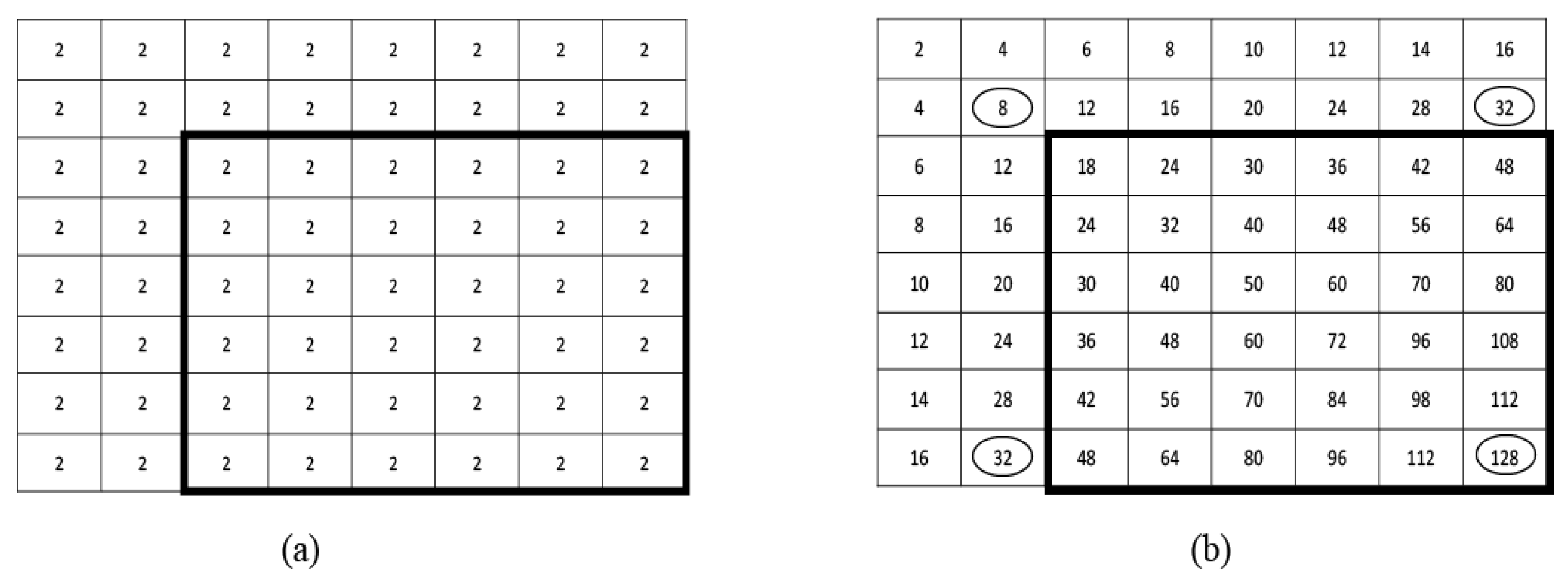
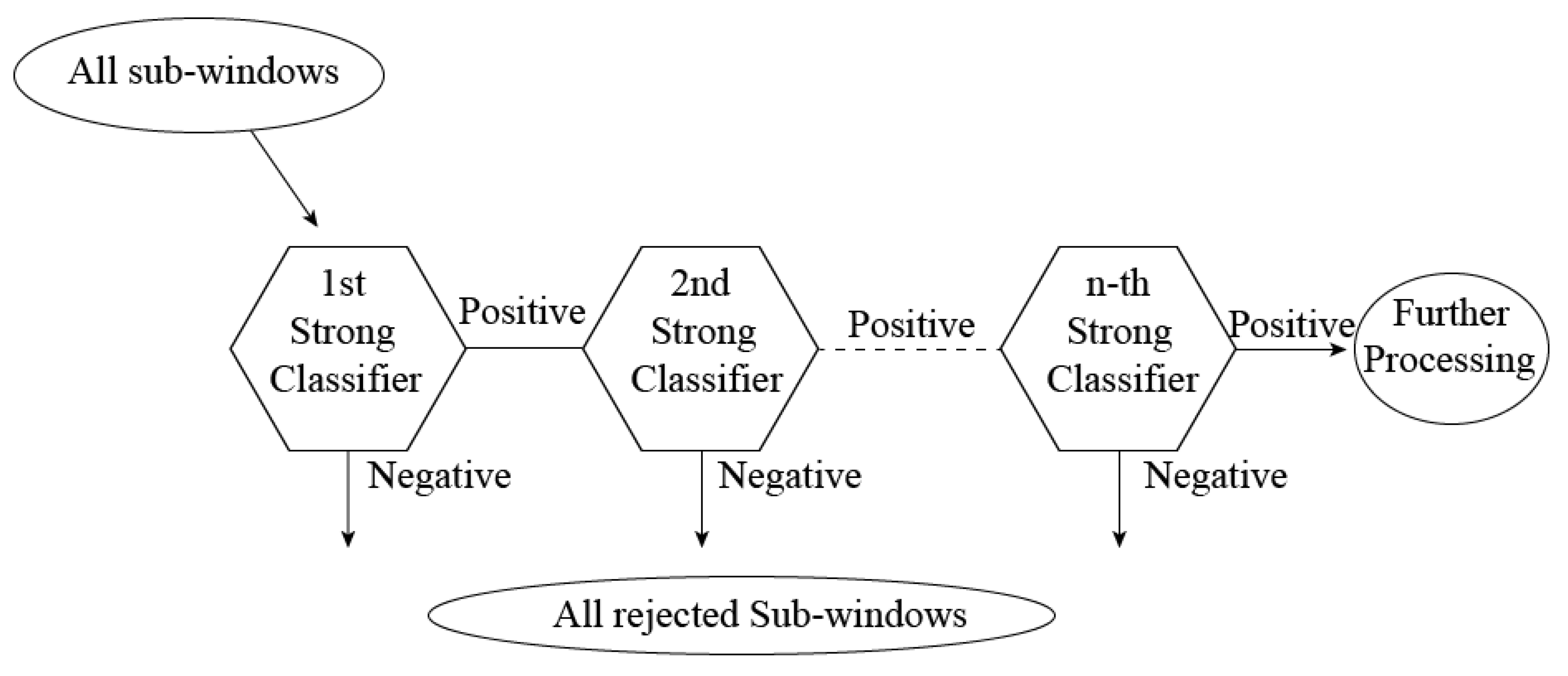
Viola–Jones Algorithm

Viola and Jones came up with an object detection framework in 2001 [41,42]. The main purpose of the framework was to solve the problem of face detection which the algorithm achieved with faster, high detection accuracy, even though the algorithm could detect a diverse class of objects. The algorithm solved problems of real-time face detection, such as slowness, computational complexity, etc.

The Viola–Jones algorithm functions in two steps: training and detection. In the detection stage, the image is converted into grayscale. The algorithms then finds the face on the grayscale image, using a box search throughout the image. After that, it finds the location in the colored image. For searching the face in a grayscale image, Haar-like features are used to search an image [43]. All human faces consist of the same features, and Haar-like features explores this similarity by making three types of Haar features for the face, namely edges, line and four-sided features. With the help of these, a value for each feature of the face is calculated. An integral image is made out of them and compared very quickly, as shown in Figure 6. An integral image is what makes this model faster because it reduces the computation costs by reducing number of array references, as shown in Figure 7. In the second stage, a boosting algorithm named the Adaboost learning algorithm is employed to select a few number of prominent features out of large set to make the detection efficient. A simplified version was delineated by Viola and Jones in 2003 [44]. Finally, a cascaded classifier is assigned to quickly reject non-face images in which prominent facial features selected by boosting are absent, as shown in Figure 8.

The Viola–Jones algorithm has high detection accuracy, and at the time of release it was reported to be 95%. A very recent study by Jamal et al. [110] reported to have 97.88% face detection accuracy. The algorithm is most widely used for face detection for its shorter computation time [111]. The algorithm is extremely successful for its low false positive rate. The algorithm was 15% quicker than the existing algorithms at the time of release. However, the algorithm can only detect the frontal side of the face. The algorithm possesses an intensely larger training time. Training with a limited number of classifiers can result in far less accurate results; a number of sub-windows was provided with more attention [112].

Rahman and Zayed presented the Viola–Jones algorithm in detecting ground penetrating radar (GPR) profiles in bridge deck [113]. The method is utilized in the detection of hyperbolic regions acquired from GPR scans. The framework lacks different clustering approaches, which would be suitable in this purpose. Huang et al. [114] proposed an improved Viola–Jones algorithm to detect faces in Microsoft Hololens. In comparison with FACE API, the speed of the local detection is 4 times and 20 times via network, but can handle a rotation of ${45}^{\circ }$. Winarno et al. [115] built face counter to count faces in an image, using the Viola–Jones algorithm. The model resulted in poor accuracy in images with low light intensity. Kirana et al. [116] proposed the Viola–Jones algorithm in the application of emotion recognition. The model was made for learning environments, such as a school. One predicament of the model is that it only works on forward-facing faces. Kirana et al. [117] extended the emotion recognition model [116] for fisher face type images. Feature extraction was performed, using PCA and linear discriminant analysis, and then combined with Viola–Jones for the detection process. Nonetheless, this combined framework is 15 times slower than the original Viola–Jones algorithm. Additionally, Hasan et al. [118] implemented the Viola–Jones algorithm in drowsiness detection, which is the main problem in the brain–computer interface paradigm. The method is based on the eye detection technique. The decision of drowsiness is made depending on the eye state (open or close). Saleque et al. [119] employed the Viola–Jones algorithm in detecting Bengali license plates in motor vehicles. The framework detects single vehicle license plates with 100% accuracy, but suffers from a reduction in accuracy in detecting multiple license plates.

Local Binary Pattern (LBP) LBP was mainly proposed for monochrome still images. LBP is based on the texture analysis on images. The texture analysis model was proposed first in 1990 [45]. However, LBP was first described by Ojala et al. in 1994 [46]. LBP works robustly as a texture descriptor and was found to have significant performance boost when working with histogram of oriented gradients (HOG) [47]. There have been reported a myriad of LBP variants, for instance, spatial temporal LBP (STLBP), $ϵ$LBP, center symmetric local binary patterns (CS-LBP), spatial color binary patterns (SCBP), opponent color local binary pattern (OC-LBP), double local binary pattern (DLBP), uniform local binary pattern (ULBP), local SVD binary pattern (LSVD-BP), etc. [120].

LBP looks for nine pixels at a time of an image—to be exact, a $3\times 3$ matrix—and particularly puts interest in the central pixel. LBP compares the central pixel (cp) with its neighboring pixel (np) and assigns 0 for np < cp and 1 for np > cp in the corresponding neighbor. Then, it turns the eight binary np into one single byte which corresponds to a LBP-code or decimal number. This is done by multiplying the matrix component wise with an eight bit number representative matrix as shown in Figure 9. This decimal number is used in the training process. We are basically interested in edges; in the image, the transition from 1 to 0 and vice versa presents a change in brightness of the image. These changes are the edge descriptors. When we look at a whole image, we look for comparisons or change in pixels or brightness, and the edges are received.

LBP is tolerant of monochromatic illumination changes because LBP just compares the neighboring pixels; a change in illumination would change the comparative values, which would not result in change in values in the comparison [122]. LBP is mostly popular for its computation simplicity and fast performance. LBP can detect a moving object by subtracting the background, and has high discriminating power with a low false detection rate [123]. The algorithm yields the same detection accuracy in offline images and in real-time operation [124]. However, LBP is not invariant to rotations and high computation complexity. LBP uses only pixel difference while ignoring the magnitude information. It is not sensitive to minor adjustments in the image.

Rahim et al. developed a face recognition system by making use of feature extraction with LBP [125]. The model achieves an incredible 100% accuracy but does not work in real time. Yeon [126] implemented a face detection framework, using LBP features. The method performed faster when compared with the Haar-like features extraction method. Priya et al. [121] utilized LBP’s advantage of micro-pattern description and solved the problem of identical twin detection. LBP was also used in surface defect detection by Liu and Xue [127]. The proposed model is an improvement of the original LBP, called gradient LBP. The model exploits image sub-blocks to plunge the LBP data matrix dimensionality. Finally, it strains non-continuity of the pixels in the local area to determine the defect area. However, this method faces noise influence when employed on the image as a whole. Varghese et al. presented an extended version of LBP, named modified LBP (MOD-LBP), and showed its application in the level identification of brain MR images [128]. When compared with original LBP, using histogram-based features, Varghese et al. found MOD-LBP to be two times better. Moreover, LBP was used in pose estimation by Solai and Raajan [129]. The model proposed by Solai and Raajan divides the estimation into five parts: front, left, tight, up and down. The pose is determined according to the pitch, yaw and roll angles of the face image. Nurzynska and Smolka implemented LBP in smile veracity recognition [130]. The model efficiently classified a posed smile and spontaneous expression. The feature vector was calculated with the use of uniform LBP. Support vector machine (SVM) was used as a classifier. Zhang et al. [131] proposed a fusion approach combining histogram of oriented grading and uniform LBP feature on blocks to recognize hand gestures. In the fusion, a histogram of oriented grading features depicts the hand shape, while LBP features epitomize the hand texture. However, the fusion yields poor result for complex backgrounds, and the speed is slow. Furthermore, LBP was implemented in script identification of handwritten documents by Rajput and Ummapure [132]. Handwritten scripts written in English, Hindi, Kannada, Malayalam, Telugu and Urdu were taken into account. Nearest neighbor and SVM were used as classifiers. LBP was used to extract features from a block of images. The defined block size was $512\times 512$ pixels. However, the model did not recognize word level images.

AdaBoost “Adaptive Boosting”, which is recognized in short for AdaBoost, is the introductory pragmatic boosting algorithm; Freund and Schapire first came up with this in 1996 [48]. AdaBoost mainly centers the attention on the classification and regression problem. The main objective of this algorithm is to adapt with hard-to-classify features. The algorithm functions by combining weak classifiers and originating a strong classifier. The algorithm changes the weights of different instances. To be exact, the algorithm puts more weight on hard-to-define classifiers and less on already-sorted-out classifiers. This is how the algorithm develops a better functioning classifier.

AdaBoost contains a high degree of precision. It has achieved a wide variety of success in many fields along with image processing. The algorithm can attain almost equivalent result on classification with small amounts of adjustment. As it combines weak classifiers, a wide variety of weak classifiers can be used to generate one strong classifier [133]. However, AdaBoost requires an enormous time for training [134]. It also can be sensitive to noisy background images and currently does not support null rejection.

Peng et al. [135] proposed two extended versions of the AdaBoost-based fault diagnosis system. One version, named gentle AdaBoost, was employed in fault diagnosis for the first time by Peng et al. For binary classification, one version of gentle AdaBoost was employed, and for multi-class classification, another version named AdaBoost multi-class hamming trees (AdaBoost.MH) was used. However, both of the extended version cannot deal with imbalanced data. Aleem et al. [136] utilized AdaBoost in software bug count prediction. Yadahalli and Nighot applied AdaBoost in intrusion detection [137]. The main goal of the system is to reduce the false alarm and ameliorate the rate of detection. Bin and Lianwen proposed a two-stage boosting–based scheme along with a conventional distance-based classification algorithm [138]. The application was to recognize in handwritten Chinese similar characters. Finally, the model was compared with AdaBoost, and AdaBoost outperformed the model. Selvathi and Selvaraj proposed an automatic method to segment brain tumor tissue and classification on magnetic resonance imaging (MRI) [139]. A combination of random forest and modified AdaBoost was presented. To extract tumor tissue texture, curvelet and wavelet transform was employed. However, this framework is limited to detecting brain tumors only. Lu et al. [140] proposed an improved ensemble algorithm, AdaBoost–GA—a combination of AdaBoost and GA—for cancer gene expression data classification. The model was designed to ameliorate the diversity of base classifiers and embellish integration processes. In AdaBoost–GA, Lu et al. introduced a decision group to improve the diversity of the classifiers, but the dimension of the decision group was not increased in order to gain highest accuracy.

Gabor Feature

The Gabor filter, named after Dennis Gabor, is extensively used for edge detection [49]. It is a linear filter used for texture analysis of an image. Gabor features are constructed by applying Gabor filters on images [50]. Images have smooth regions interrupted by abrupt changes and contrast called edges. These abrupt changes or edges usually contain the most prominent information in an image and hence, can indicate the presence of a face. Fourier transform is prominent in change analysis, but is not efficient in dealing with abrupt changes. Usually, Fourier transforms are represented by sine waves oscillating in infinite time and space. However, for image analysis, there is a need for something that can be localized in finite time and space. This is why the Gabor wavelet is utilized, which is a rapidly plunging oscillation with a mean zero [55]. For detecting the edges, the wavelet is used and searched over an image, initially positioning it at a random position in the image. If no edges are detected, the wavelet is searched at a different random position [51].

Using the Gabor feature, impressive results on face detection was reported by the dynamic link architecture (DLA) [141], elastic bunch graph matching (EBGM) [142], Gabor Fisher classifier (GFC) [143], and AdaBoosted Gabor Fisher classifier (AGFC) [144]. Gabor feature analysis works well with magnitudes [145]. A large amount of information can be gathered from local image regions [146,147]. Gabor feature analysis is found to be invariant to rotation, illumination and scale [148,149,150,151]. However, Gabor feature analysis has time complexity and image quality issues.

Gabor feature analysis was employed on gait analysis by Li et al. [152]. Human gait was classified into seven components. Two types of gait recognition processes were performed; one based on an entire gait outline, and another based on certain combinations. Two applications were proposed, depending on the analysis: human identification and gender recognition. The model cannot wring out dynamic properties of walking sequence. Zhang et al. [153] proposed an improved version of Gabor feature analysis, named local Gabor binary pattern histogram sequence (LGBPHS), for face representation and recognition. The model does not need any training because of its non-statistical approach. LGBPHS comprises many parts of the histogram, corresponding to different face components at various orientations and scales. However, the framework does not handle pose and occlusion variation well enough. Cheng et al. [154] implemented Gabor feature analysis in facial expression recognition. The method is based on Gabor wavelet phase features. Conventional Gabor transformation processes utilize Gabor amplitude as a feature. Yet, Gabor amplitude features have small changes as the variation of the spatial location, while the phase can quickly change in accordance with the change in position. The presented model uses the intense texture characteristics gathered from phase information to detect facial expression. Priyadharshini et al. [155] compared Gabor and Log Gabor in vehicle recognition and proved the superiority of Log Gabor in vehicle recognition. Yakun Zhang et al. [156] presented a solution to the parameter adjustment of the Gabor filter with an application in finger vein detection. The model was named the adaptive learning Gabor filter. Additionally, a new solution for texture recognition by combining gradient descent and the convolution processing of the Gabor filter was proposed. However, the soft features available in finger veins was ignored in the process. Gabor feature analysis was utilized in fabric detection by Han and Zhang [157]. A GA algorithm was proposed to use, jointly, in determining the optimal parameters of the Gabor filter, depending on the defect-free fabric image. The model yields positive results on defects of various shapes, sizes, types. Rahman et al. applied Gabor feature analysis in the detection of the pectoral muscle boundary [158]. The model tunes the Gabor filter in the direction of the muscle boundary on the region of interest (ROI) containing the pectoral muscle. After that, it calculates the magnitude and phase responses. The responses calculated with the edge connect and region merge are then utilized for the detection process.

2.3.2. Constellation Analysis

Constellation is a cluster of similar things. In a constellation analysis, a facial feature group is formed to search a face in an image [52,53]. The algorithm is free from rigidity. This is why it can detect faces in images with noisy backgrounds. Most of the algorithms reviewed before failed to perform face detection in images with a complex background. Using the facial features, a face constellation model solved this very problem easily.

Various types of face constellations have been proposed by numerous scientists. We discuss three of them: statistical shape theory by Burl et al. [54], probabilistic shape model by Yow and Cipolla et al. [56] and graph matching. Statistical shape theory has a success rate of 84% and it can operate smoothly with features that are missing. The algorithm handles properly the problems originated from rotation, scale and translation to a certain magnitude. However, a significant amount of rotation in the subject’s head causes a severe problem in detection. On the other hand, the probabilistic shape model marks a plunge in the detection of invalid features from noisy image and illustrates a 92% accuracy. The algorithm handles minor variations in viewpoint, scale and orientation. Additionally, eye glasses and missing features do not generate any problems. Lastly, graph matching can perform face detection in an automatic system and has higher detection accuracy.

Constellation analysis has been effectively used in telecommunication [159], diagnostic monitoring [160] and in autonomous satellite monitoring [161]. The similarities and differences among different FA are epitomized in

Table 4. Comparison of different FA.

		Feature Analysis
		FS [38,39,40]	CA [52,53]
Similarities	Problem in getting feature positions correct	✓	✓
	Works well on cluttered background	✓	✓
Differences	Reference	Head, mouth, ears, eyes	Eyeballs, distance between eyes
	Pre-conditions	Can handle variable illuminations and brightness	Working range 10 to 74 pixels and −30 to +30 degrees

.

3. Image-Based Approaches

Detecting faces on a more cluttered backgrounds paved the the way for most image-based approaches. Most of the image-based face detection techniques work by using window-based scanning. The window is scanned pixel by pixel to classify a face and non-face. Typically, every method in image-based approaches varies in terms of the scanning window, step size, iteration number and sub-sampling rate to produce a more efficient approach. Image-based approaches are the most recent techniques that have emerged in face detection and are classified into three major fields: neural networks, linear subspace methods and statistical approaches as shown in Figure 10.

3.1. Neural Network

Neural network algorithms are inspired by the human brain’s biological neural network. Neural networks take in data and train themselves to recognize the pattern (for face detection the face pattern). Then, the networks predict the output for a new set of similar faces. Neural networks can be subdivided into artificial neural network (ANN), decision-based neural network (DBNN) and fuzzy neural network (FNN).

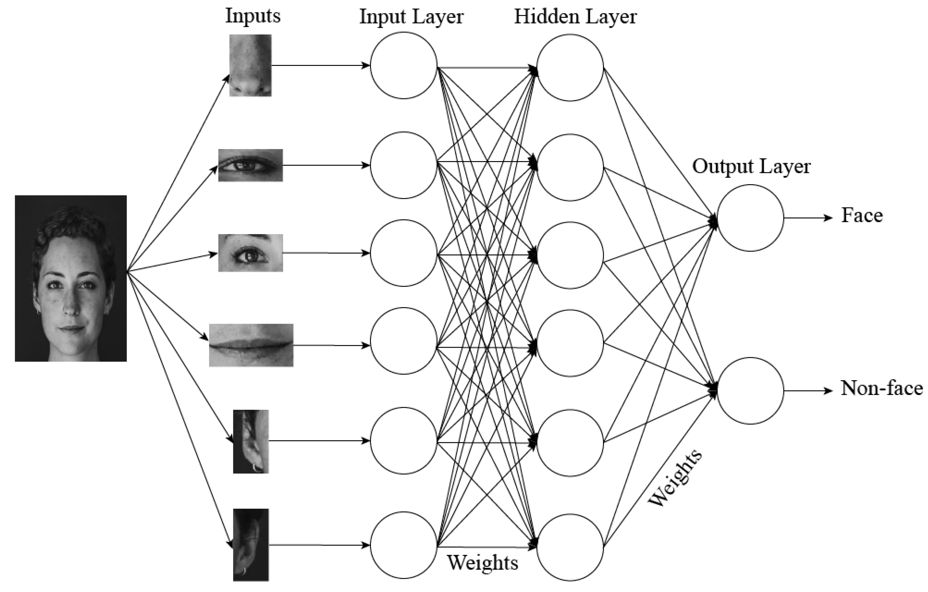
3.1.1. Artificial Neural Network (ANN)

Like the biological human brain, ANN is based on a collection of connected nodes. The connected nodes are called artificial neurons. The fact of learning patterns in data enables ANN to produce better results with the availability of more data. There are several numbers of ANNs available. The most popularly used ANNs in face detection are added below.

Retinal Connected Neural Network (RCNN)

A neural network based on the retinal connection of human eyes was proposed by Rowley, Baluja and Kanade et al. in 1998 [162]. The proposed ANN was named the retinal connected neural network (RCNN). RCNN takes a small-scale frame of the main image to analyze whether the frame contains a face as shown in Figure 11. RCNN applies a filter on an image. The filter is based on the neural network. A temporary arbitrator is used to merge the output to a single node. The input image is searched thoroughly, applying a different scale of frame to search for face content. The output node, with the help of an arbitrator, eliminates the overlapping features and combines the face features gathered from filtering.

RCNN can handle a wide variety of images with different poses and rotation. When using RCNN, the methodology can be sorted out to be more or less conservative depending on the arbitration heuristics or thresholds used. The algorithm reports an acceptable number of false positives. However, the procedure is complex in terms of implementing and can only encounter frontal faces looking at the camera.

Feed Forward Neural Network (FFNN)

The feed forward neural network (FFNN), also known as multi-layer perception, is considered to be the simplest form of ANN. The neural network was upheld from perceptrons developed by Frank Posenblatt et al. in 1958 [163]. Perceptrons are methodologies of the brain to store and organize information. Information or, for images, the face feature information moves to output nodes from input nodes, where the movement is done via hidden layers. Hidden layers assign weights to face features on the training process as shown in Figure 12. In the detection stage, the weights are compared to report a result on a given image. FFNN can handle large tasks, and accuracy is only higher on training samples.

Ertugrul et al. employed FFNN in estimating the short term power load of a small house [194]. The proposed model is a randomized FFNN. A small grid dataset was used in the evaluation and validation process. However, total accuracy dropped because of the bias in the output layer. Chaturvedi et al. [195] applied the FFNN and Izhikevich neuron model in the handwritten pattern recognition of digits and special characters. A comparison between both of them was made and it was proved that by adjusting synaptic weights and threshold values, the input patterns can achieve the same firing rate. Additionally, FFNN was implemented in image denoising by Saikia and Sarma [196]. The proposed method is a combination of FFNN and multi-level discrete cosine transform. The fusion manages speckle noise, which is a kind of multiplicative noise generated in images. Mikaeil et al. proposed FFNN in low latency traffic estimation [197]. The framework shows significant improvement in utilization performance, upstream delay and packet loss handling. Dhanaseely et al. [164] presented FFNN and cascade neural network (CASNN) in face recognition. Feature extraction was performed, using PCA, and Olivetti Research Lab (ORL) database was utilized. Both models were compared after the recognition process and it was found that CASNN is better in this scenario.

Back Propagation Neural Network (BPNN)

The origin of BPNN has some misleading information. Despite this fact, Steinbunch et al. proposed a learning matrix in 1963 [164]. This is one of the earliest involvement with BPNN [198]. A modern updated version was developed by Seppo et al. in 1975 [199]. The version is also called reverse mode automatic differentiation (RMAD). BPNN came into attention after the release of a paper by Rumelhart, Hinton and Williams in 1986 [165].

BPNN implements a system called “learning by example". BPNN calculates the error back in the input from the output to adjust the weights in the hidden layer for more accurate output. A number of face features are used as input in the training stage. A larger amount of weights are assigned to every features and compared with input nodes with errors. If the error rate is higher, the weight value is decreased on the next attempt and compared with the input node again. Thus, minimal error reporting weights are generated and employed in the detection stage for new images given. The face features are calculated using the predicted weights.

BPNN is fast, easy to program and simple to implement. The algorithm does notneed any special mention of the features of the function to be learned. BPNN is also flexible without the need for any prior knowledge about the network. Furthermore, the algorithm has no input parameter, except the input number. However, BPNN faces the major disadvantage of getting stuck into local minima.

Chanda et al. [200] applied BPNN in plant disease identification and classification. In order to fight overfitting and local optima, the framework utilizes BPNN to obtain the weight coefficient and particle swarm optimization (PSO) for optimization. The model implements five pre-processing steps: resizing, contrast enhancement, green pixel masking, and color model transformation. Finally, image segmentation is performed to classify te diseased portions of the plant. However, the model faces problems in choosing the initial parameter values of PSO. Yu et al. [201] implemented BPNN in tooth decay diagnosis. The model takes input the X-ray images of the patient’s teeth. Normalized autocorrelation coefficients were employed to classify decayed and normal teeth. Additionally, BPNN was used in data pattern recognition by Dilruba et al. [202]. The model aims at finding the match ratio of training patterns to testing patterns. Two types were taken as a match: one is an exact match and the other is almost similar pattern. Li et al. utilized BPNN in building a ship equipment fault grade assessment model [203]. Three types of BPNN were taken into account: gradient descent back propagation algorithm, momentum gradient descent back propagation algorithm and Levenberg–Marquard backpropagation algorithm. To quantify the initial weight value of the neural network, GA is employed. Finally, a comparison among the three BPNN shows that Levenberg–Marquard backpropagation outperforms the other two. Furthermore, BPNN was employed in the analysis of an intrusion detection system by Jaiganesh et al. [204]. The framework analyses the user behavior and classifies them as normal or attack. The model yields poor attack detection accuracy.

Radial Basis Function Neural Network (RBFNN)

The radial basis function neural network (RBFNN) was presented by Broomhead and Lowe in 1988 [166,205]. RBFNN has similarities structurally with BPNN. RBFNN is comprised of input, hidden and output layers. However, RBFNN has only one hidden layer, and it is strictly bounded to only one hidden layer, named the feature vector. When mapping or neuron activating, RBFNN makes use of the Gaussian potential function.

In RBFNN, computations are relatively easy [167]. The network can be trained, using the first two stages of the training algorithm. The network possesses the property of best approximation [206]. The ANN shows easy design and strong tolerance to input noise, online learning ability and good generalization [207]. Additionally, RBFNN has a flexible control system. Despite those, an inadequate number of neurons in the hidden layer results in the failure of the system [208]. Additionally, a large number of neurons can result in overlapping in RBFNN.

Karayiannis and Xiong implemented an extended version of RBFNN, named cosine RBFNN, in identifying uncertainty in data classification [209]. The model was built by expanding the concepts behind the design and training of quantum neural networks (QNN), which is capable of detecting uncertainty in data classification by themselves. This method yields a learning algorithm that fits the cosine RBFNN. In the field of data mining, RBFNN was employed by Zhou et al. [210]. To speed up the learning process, a two-stage learning technique was used. To increase the output accuracy of the RBFNN, an error correlation algorithm was proposed. Static and dynamic hidden layer architecture was suggested to build a better structure of hidden layers. Venkateswarlu et al. [211] applied RBFNN in speech recognition. The framework is suitable in recognizing isolated words. Word recognition was performed in a speaker-dependent mode. When compared to multilayer perceptron neural networks (MLP), it improves efficiency significantly. Guangying and Yue employed RBFNN in the study of an electrocardiograph [212]. For the construction of RBFNN, a new algorithm was introduced. The proposed model generalizes on the given input well. The framework shows great efficiency in electrocardiogram (ECG) feature extraction. The model only considers two basic cardiac actions, despite the fact that cardiac activity is far more complex.

Rotation Invariant Neural Network (RINN)

Rowley, Baluja and Kanade proposed rotation invariant neural network (RINN) in 1997 [168]. Conventional algorithms are restricted to detecting frontal face only, while RINN can detect faces at any angle of rotation. The RINN system consists of manifold networks. At the beginning, a network name router network holds every input network to find its orientation. After that, the network prepares the window to detect one or more detector networks. The detector network processes the image plane to search for a face.

RINN can handle an image at any degree of rotation. RINN displays a higher classification performance [169]. Even so, RINN can learn only a limited number of features and performs well only with a small number of training sets.

RINN was implemented in coin recognition [213] and in estimating the rotation angle of any object in an image [214]. Additionally, RINN was also exploited in pattern recognition [215].

Fast Neural Network (FNN)

The fast neural network (FNN), which reduces the computation time of the neural network, was first presented by Hazem El-Bakry et al. in 2002 [170]. FNN is very fast in computing and detecting human faces in an image plan. FNN works by diving an image into sub-images. Each of the sub-images are then searched for a face or faces, using the fast ANN or FNN. A high speed in detecting faces was reported when using FNN.

FNN reduces the computation steps in detecting a face [170]. In FNN, the problem of sub-image centering and normalization in the Fourier space is solved. FNN is a high-speed neural network, and parallel processing is implemented in the system. Yet, FNN is reported to be computationally expensive. FNN can be implemented in object detection besides face detection [170].

Polynomial Neural Network (PNN)

Haung et al. presented the polynomial neural network (PNN)–based face detection technique in 2003 [171]. PNN was originally proposed by Ivakhnenko in 1971 [172,216]. The algorithm is also known as group methods of data handling (GMDH). The GMDH neuron has two inputs and one output, which is a quadratic combinations of two inputs.

To detect a face, a frame that can slide over an image is introduced, and the detector labels the frames that contain a face. The test image is divided into variable scales to examine the numerous face shapes. The dividing process is actually re-scaling the input image into a standard frame. To overcome overlapping due to the re-scaling and multiple faces in the detection region, the images are arbitrated. The lighting conditions are ratified with an optimal plane, causing minimal error, and pixel intensities are fixed to compose a feature vector of 368 measurements. The classifier PNN, which has a single output, detects a window with a face or non-face. The complexity is slumped by PCA. PCA also helps to improve efficiency.

PNN can handle images with a cluttered background. Additionally, the algorithm is reported to have a high detection rate and low false positive rate in images with both simple and complex backgrounds. However, the algorithm is reported to have suffered from overlapping in the images output, due to re-scaling. The algorithm can also cause a problem in detecting faces in an image with a large number of faces in it.

PNN was implemented in signal processing with a chaotic background by Gardner [217]. The model generates a global chaotic background prediction, which is then subtracted to improve the signal. Ridge PNN (RPNN), an extended version of PNN, is a non-linear prediction model developed by Ghazali et al. [218] to forecast the future patterns of financial time series. The model was also extended to another version in the same paper as the dynamic ridge polynomial neural network (DRPNN), which is almost similar to the feed forward RPNN, with a feedback connection as the difference. Over and above that, PNN was put into action in gesture learning and recognition by Zhiqi [219]. The activation function is a Chebyshev polynomial, and the weights of the neural network are obtained by using a direct approach based on the pseudo-inverse. The procedure cuts down on training time. It also boosts precision and generalization. Furthermore, PNN was employed in the modeling of switched reluctance motors by Vejian et al. [220]. The model is used to simulate the flux linkage and torque characteristics of switched reluctance motors mathematically. The most appealing aspect of this is that it is self-adaptive and does not depend on a priori mathematical models.

Convolutional Neural Network (CNN)

There are many debates over who was the first to present the convolutional neural network (CNN). Despite much argument, most literature review and studies refer to some papers of LeCun et al. from 1988 to 1998 [173,221]. CNN was implemented in many research works on face detection. Some early contributions are the proposed works of Lawrence in 1996 [222], in 1997 [223] and Matsugu in 2003 [174].

CNN has a structure almost similar to FFNN. Hence, CNN has convolutional and some other layers consisting of hidden layers; for convolutions in the hidden layers, CNN is named as such. In convolutional layers, an input is convoluted and then passed to the next layer. We should define filters in the convolution layer. To sum up the process, the training stage trains the network, and best weighted values or filters are saved for detection. The network is trained with the usual backpropagation gradient descent procedure [222]. In the detection stage, the filters are scanned over the image to find patterns. Patterns can be edges, shapes or the colors.

For a completely new task, CNN is a very good feature extractor. Additionally, CNN shows a very high computational efficiency and high accuracy. However, CNN requires big dataset for proper training. CNN reports to be slow and holds a high computational cost.

Besides face detection, CNN was also employed in improving bug localization by Xiao and Keung [224]. Bug reports and source files were reviewed on a character-by-character basis rather than a word-by-word basis. To extract features, a character level CNN was used, and the output was fed into a recurrent neural network (RNN) encoder–decoder. However, no fine tuning was performed in the model. Mahajan et al. applied CNN in the prediction of fault in gas chromatographs [225]. The fault was predicted by abnormalities in the pattern of the gas chromatogram, according to the model. Shoulder top, negative peak, and good peak faults were all successfully established. In spite of them, the model training lacked an adequate dataset. Hu and Lee proposed a new time transition layer that models variable temporal convolution kernel depths, using improved 3D CNN [226]. The model was also improved by adding an extended DenseNet architecture with 3D filters and pooling kernels. The model also added a cost-effective method of transferring pre-trained data from a 2D CNN to a random 3D CNN for appropriate weight initialization. CNN was employed in node identification in wireless network by Shen and Wang [227]. The dimension of every node was downsized, using PCA. Local features were extracted, using two layers CNN. For optimizing the model, stochastic gradient descent was utilized. To execute, the decision output softmax model was employed. The model performs poorly on larger scale networks. Shalini et al. conducted a sentiment analysis of Indian languages, using CNN [228]. The dataset used contained Telugu and Bengali languages. Data were classified as positive, negative and neutral. The model was implemented, using just one hidden layer. However, the model had a low cross validation accuracy for Telugu data.

3.1.2. Decision-Based Neural Network (DBNN)

Kung et al. presented an eminent face detection algorithm based on the decision-based neural network (DBNN) in 1995 [175]. DBNN uses static process for still images and a temporal strategy for video. In the training stage, the face pattern was annealed in order to make the eye plane horizontal and to produce a structure where distance between the eyes are constant. A Sobel edge map was assembled of size 16 by 16 pixels from images containing either a face or non-face. The Sobel edge map was later used as an input to the DBNN. The sub-images were processed to find face shapes in them. The face pattern was then located in the sub-image of the main frame it corresponds to. When the whole image is considered, only the found sub-image containing face is located as the desired location of the face.

DBNN is very effective in computation performance and time [229]. The hierarchical structure of DBNN provides a better understanding of structural richness. Furthermore, DBNN is reported to have high recognition accuracy, and its processing speed is very high (less than 0.2 second). However, the detection rate is higher only when the facial orientation is between −15 and 15 degrees.

Kung et al. applied DBNN in palm recognition [175]. The model classified palms as one being from the database or an intruder. The main drawback is the use of a small dataset. Application in image and signal classification task of DBNN was proposed by Kung and Taur [229]. The model was a fusion of the learning rule of perceptron and hierarchical non-linear network structure. A sub-clustering hierarchical DBNN was explored for static models, and a fixed weight low pass filter was used for temporal prediction models. Golomb et al. implemented DBNN in gender classification [230]. The model does not necessitate function selection and optimization beforehand. The model requires complex calculations for simplistic classification.

3.1.3. Fuzzy Neural Network (FNN)

An intelligent system, which is the combination of the human-like reasoning style of a fuzzy system with the learning and connection-establishing structure of the neural network, is known as neuro-fuzzy hybridization. Neuro-fuzzy hybridization is eminently called the fuzzy neural network (FNN). FNN was employed in face detection by many researchers. Among them, Rhee et al. in 2001 [176], Bhattacharjee et al. in 2009 [231], Petrosino et al. in 2010 [232], Pankaj et al. in 2011 [233] and Chandrashekhar et al. in 2017 [177] implemented FNN in face detection.

To begin with, the pre-processed $20\times 20$ frame, either containing a face or not, are allocated by fuzzy membership degrees. These fuzzy membership degrees are then used as an input to the neural network. The neural network is trained by the degrees, using error back propagation. When the training is over, an evaluation is run over the network, which defines the degree of which a given window contains a face or not. If a frame is labeled to have a face, post-processing is then carried out.

FNN is reported to have an higher accuracy, compared to other neural networks [176]. FNN requires fewer hidden neurons and can handle noisy backgrounds. Despite these, the FNN system requires linguistic rules instead of learning by examples as prior knowledge [234].

Kandel et al. [235] proposed a more adaptive FNN in pattern recognition. The model applies GA to the Kwan–Cai FNN. The number of Fuzzy neurons is lowered, and the recognition rates are enhanced, using a self-organizing learning algorithm based on GA. However, only English letters and Arabic numerals were used to evaluate the model. Imasaki et al. [236] utilized FNN to fine-tune the elevator’s performance. The FNN-trained system is capable of adapting to a variety of traffic circumstances. Long-term shifts in traffic situations are handled by the model. Even so, the system must be customized to meet the needs of the users. Furthermore, FNN was employed in building the control system of automatic train operation by Sekine et al. [237]. Sekine et al. suggested a fuzzy neural network control scheme with two degrees of freedom. The model depicts the use of fuzzy rules both before and after the process begins. It also decreases the number of fuzzy rules that must be used. Despite changes in the control purpose and complex characteristics, automated operation continues to function well. Lin et al. presented an extended FNN named interactively recurrent self-evolving fuzzy neural network (IRSFNN) in identifying and predicting a dynamic system [238]. To maximize the benefits of local and global feedback, a novel recurrent structure with interaction feedback was introduced. A variable-dimensional Kalman filter algorithm was used to tune IRSFNN. Xu et al. [239] applied FNN in pulse pattern recognition. According to traditional Chinese pulse diagnosis (TCPD) theory, the model used FNN as a classifier to classify pulse patterns. The model has a high level of accuracy. Nonetheless, it is unable to detect complex pulse patterns, due to the limitations of the pulse dataset. Comparisons among different NN are listed in

Table 5. Comparison of different NN.

		Neural Network
		ANN [167,169,207]	DBFN [175,229]	FNN [231,232]
Similarities	Use gradient for weight update	✓	✓	✓
	Low error rate	✓	✓	✓
Differences	Complex background, uncontrolled illumination	Strong tolerance	Performance degraded	High detection rate
	Combination	Error back propagation	Perceptron like learning + hierarchical Non-linear rule	Fuzzy logic + Neural connection rule

.

3.2. Linear Subspace

The linear subspace is a vector space, which is a subset of a larger vector space. In image processing terms, the smaller portion of a frame is called a subspace. The linear subspace is classified into four groups, i.e., eigenfaces, probabilistic eigenspaces, Fisherfaces and tensorfaces.

3.2.1. Eigenfaces

Sirovich and Kirby first proposed the use of eigenfaces in face analysis [178,240], which was implemented in face recognition by Truk and Pentland [23,179].

The main goal of face detection is finding the faces in a given input image. The images that are used as an input are usually highly noisy. The noise is created due to the pose, rotation, lighting conditions, and other invariants. Despite the noises, there are some patterns that exist in an image. The image containing a face usually consists of patterns, due to the presence of some facial objects (eyes, noses, etc.). These facial features are called eigenfaces. These are usually obtained from an image by PCA. Using PCA, an eigenface of corresponding features are constructed from training a set.

By combining all the eigenfaces in the right proportion, the original face can be rebuilt. Each eigenface stands in for a single feature of a face. All the eigenfaces may or may not be available in an image. If a feature is present in an image, the proportion of the feature in the sum of eigenfaces will be higher. Therefore, a sum of all the weighted eigenfaces will represent a full face image. The weight defines in what proportion a feature is present in the image. That is, the reconstructed original image is equal to a sum of all the eigenfaces, with each eigenface having a certain weight. This is how a face, using the weighted eigenspaces, is extracted from an image.

The eigenface approach requires no knowledge of geometry and reflectance of faces. Furthermore, data compression is achieved by the low-dimensional subspace representation. However, the approach is very sensitive to the scaling of the image. Additionally, the learning or training stage is very time consuming and shows efficiency only in the condition that face classes are larger in dimension, compared to face spaces.

Along with face detection, the method was used in speaker identification by Islam et al. [241]. The model categorizes speakers based on the content of their voice. For feature extraction, the Fourier spectrum and PCA approaches were used. The classification is then done, using eigenface. The system recognizes the speaker based on every word spoken by the speaker. The system’s biggest flaw is that it does not operate in real time. Zhan et al. [242] used the eigenface approach for real-time face authentication. The main contribution of this method is the 3D real-time face recognition system. The intensity and depth maps, which are continuously collected, using correlation image sensor (CIS), are used to classify the data. The complex valued eigenface is added to the traditional eigenface. Many potential applications, such as face emotion detection and attractiveness detection, are not discussed in this paper.

3.2.2. Probabilistic Eigenspaces

The eigenface approach for face detection obtained impressive results in a constrained environment. Hence, this technique performs well on only rigid faces. On the other hand, probabilistic eigenspaces proposed by Moghaddam and Pentland [180,243] implements a probabilistic similarity measure, based on a parametric estimate of the probability density.

The method is reported to handle a much higher degree of occlusion [181]. Furthermore, the probability distribution of the reconstruction error of each class was employed, and the distribution of the class members in the eigenspace was taken into consideration [244].

3.2.3. Fisherfaces

Belhumeur, Hespanha and Kriegman proposed Fisherface for face detection in 1997 [182]. One key problem in face detection is finding the proper data representation. PCA by finding eigenfaces solves this problem. So, the subspace in an image representing the most of the variance or face can be described by eigenfaces. However, the similarity in the face subspace is not clearly defined by eigenfaces. In such situations, a subspace that gathers the same classes in one spot and those that are dissimilar far apart is required. The process to achieve the tasks is called discriminant analysis (DA). The most popular DA is linear discriminant analysis (LDA). LDA is implemented to search for a facial subspace, which is called Fisherface.

The algorithm is very useful when facial images have large variations in illumination and facial expression. Additionally, the error rate in detecting faces with glass is very small compared to the eigenface. Furthermore, Fisherfaces require less computation time than eigenfaces. However, Fisherfaces heavily depend on input data.

Jin et al. used Fisherfaces in automatic modulation recognition of digital signals [245]. The model focused on reducing dimensionality based on Fisherfaces. It also used a combination of the cyclic spectrum and k-nearest neighbor to recognize nine different types of modulation signals. Du et al. combined Fisherfaces and the fuzzy iterative self-organizing technique to recognize gender, using human faces [246]. Fisherface was used to extract relevant attributes, which were then clustered, using a fuzzy iterative self-organizing technique. The fuzzy nearest neighbor method was then used to classify the data. Additionally, the algorithm was utilized in classifying facial expression by Hegde et al. [247]. The output of different blocksizes was analyzed, using the Gaussian adaptive threshold process. Fisherface was employed to detect different human emotions. The model also used eigenface and local binary pattern histogram (LBPH) to reduce differences between classes within an image, such as varying lighting conditions. The process maximizes the mean difference between groups, allowing it to accurately distinguish between individuals.

3.2.4. Tensorfaces

Tensorfaces was presented by Vasilescu and Terxopoulos in 2002 [183,184]. Tensorfaces is a multilinear approach where a tensor is a generalization of a matrix in a multidimensional basis. An image is dominated with multiple factors such as structure, illumination and viewpoint. The solution of the problems along with a band of images remains in the multilinear algebra domain. Within this mathematical method, a higher dimensional tensor is used to represent an image ensemble. To find faces by decomposing the images, an extension of singular value decomposition (SVD) named N-mode SVD is employed. The N-mode SVD yields tensorfaces from an image.

Tensorfaces can be implemented as an unified framework for solving several computer vision problems. Furthermore, the performance of tensorfaces was reported to be significantly better, compared to eigenfaces.

Table 6. Comparison of different LSM.

		Linear Subspace Methods
		Eigenface [178,179,240]	Probabilistic Eigenspace [180,243]	Fisherfaces [182]	Tensorfaces [183,184]
Similarities	Works well on members of ensemble	✓	✓	✓	✓
	Works ideally on specified frame	✓	✓	✓	✓
Differences	Subspace finding	PCA	Eigenspace decomposition	LDA	N-mode SVD
	Insensitive	Small or gradual change in face image	Rigid faces	Lighting and facial expressions	Scene, structure, illumination, viewpoint

enlists comparisons among different LSM.

3.3. Statistical Approaches

Among various face detection methods, statistical approaches are the most intensively studied topic. The major sub-areas in the field are principal component analysis (PCA), support vector machine (SVM), discrete cosine transform (DCT), locality preserving projection (LPP) and independent component analysis (ICA).

3.3.1. Principle Component Analysis (PCA)

PCA was first proposed by Karl Pearson in 1901 [185], and was later advanced and named by Harold Hotelling in 1933 [186].On the basis of field application, PCA is known by several names, such as proper orthogonal decomposition (POD) in mechanical engineering, Kerhunen–Loeve transform (KLT) in signal processing, and so on. Turk and Pentland first implemented PCA in face detection.

PCA compresses a lot of data into some captures of the essence of real data. The mathematical procedure that PCA uses is an orthogonal transformation to convert a set of values of possibly correlated M variables to a set of K uncorrelated variables, called principal components. The components are gathered from the training set and only the first few components are obtained, while others are rejected. The obtained components are also called eigenfaces. The detection of a face is performed by projecting a test image onto a subspace spanned by the eigenspaces.

PCA performs very well in a constrained environment, and it is reported to be faster than other statistical approaches. An improved statistical-PCA (SPCA) is delineated to have a high recognition rate and simple computation [248,249]. However, PCA only relies on linear assumptions and scale variants.

PCA was employed also in cancer molecular pattern discovery by Han in [250]. Han introduced a non-negative PCA variant of PCA, which added non-negative constraints to PCA. As a classifier, the model employs SVM. The NPCA-SVM model was created by combining the two models. Under a regular Gaussian kernel, the model overcomes overfitting associated with SVM-based learning machines. Convergence issues can arise when using the model as a result of using a fixed phase size. Additionally, PCA was utilized in water quality monitoring [251]. Bingbing [252] implemented PCA in noise removal for speech denoising. Using dynamic embedded technology, the architecture produced an embedded matrix. The main components were then converted, using PCA. Finally, the model rebuilt the speech with no noise (high order principle components), using low order principle components. Tarvainen et al. [253] applied PCA in cardiac autonomic neuropathy. Instead of conforming to a small range, the model used multi-dimensional heart rate variability (HRV). Then, for dimensionality reduction, PCA was used, allowing the HRV to model the majority of the details in the original multi-dimensional data. Ying et al. [254] used PCA in building model for fire accidents of electric bicycles. The main drawback is limitation of fire data from actual fire incidents.

3.3.2. Support Vector Machine (SVM)

SVM is the modification of the generalized portrait algorithm, which was introduced by Vapnik and Lerner in 1963 [187]. Vapnik and Chervonenkis further developed the generalized portrait algorithm in 1964 [255]. The closer form of SVM currently used popularly was proposed by Boser, Guyon and Vapnik in 1992 [256]. SVM was used in face detection by many researchers in recent times [188,257,258,259,260,261].

In the training stage, features are extracted using PCA or Histogram of Oriented Grading (HOG) or other feature extraction algorithms. Using the data, SVM is trained to classify between a face and a non-face. It draws a hyperplane between the classes as shown in Figure 13. In the detection stage, the received frame is extracted and compared with trained images put into the specific class of a face or a non-face.

SVM is reported to be very effective with higher dimensional data. Furthermore, SVM models have generalization in practice; thus, the risk of over-fitting is quite small in SVM. SVM is reported to be memory efficient as well. However, SVM is not suitable for a large dataset. It works poorly with a noisy image dataset [262].

SVM was effectively utilized in protein structure prediction by Wang et al. [263] and in physical activity recognition by Mamun et al. [264]. Moreover, SVM was reported to be successful in breast cancer diagnosis by Gao and Li [265]. The model analyzed data using various kernel functions and SVM parameters. The radial basis function kernel and polynomial kernel were used to achieve the highest accuracy. Nasien et al. [266] applied SVM in handwritten recognition. The skeleton of a character was extracted, using a thinning algorithm. To accurately reflect the characters, a heuristic was used to generate Freeman chain code (FCC). The model yielded high accuracy. The proposed system, however, relied solely on the National Institute of Standards and Technology (NIST) database, which contains low-quality samples and broken bits. Gao et al. [267] implemented SVM in intrusion detection. They employed GA to optimize the SVM parameters. Menori and Munir combined blind steganalysis and SVM to detect hidden message and estimate hidden message length [268]. Among the different used kernels in the system, the polynomial kernel performs best.

3.3.3. Discrete Cosine Transform (DCT)

DCT was first proposed by Nasir Ahmed et al. in 1974 [189]. DCT was invented to perform the task of image compression [269,270]. DCT was used in face detection and recognition by Ziad et al. in 2001 [271], Aman et al. in 2011 [190], Surya et al. in 2012 [272], and so on.

The position of the eyes in an image needs to be entered manually. This is not considered a major drawback of the algorithm, as the algorithm can be used with a localization system [190]. After the system receives an image and eye coordinates in it, geometric and illumination normalization is performed. Then, the DCT of the normalized face is computed, and a certain subset of DCT coefficients describing the face is held onto as a feature vector. These subsets of DCT coefficients hold the highest variance of the image, which are of low to mid frequency. To detect and recognize a face, the system compares this face feature vector with the feature vectors of the database faces.

DCT was reported to show significantly vast improvement in the detection rates because of normalization and to be computationally less expensive, compared to Karhunen–Loeve transform (KLT) [190]. In addition, DCT provides a simpler way to deal with 3D facial distortions and produces rich information of face descriptors [273]. Even so, quantization (ignoring high frequency components) is required to make some decisions in DCT. DCT was also used in audio signal processing, fingerprint detection, palm print detection, data compression, medical technology, and wireless technology [274].

3.3.4. Locality Preserving Projection (LPP)

Ha and Niyogi proposed LPP in 2004 [191]. The algorithm can be used as a substitute for PCA. LPP was developed to store locality structure which makes LPP fast as pattern recognition algorithms explores nearest patterns.

In LPP, like PCA, a face subspace is searched, which usually has lower dimensions than the image space [275]. The original image is put under scale and orientation normalization. The normalization is performed in such a way that two eyes were aligned at the same position. Then, the image is cropped into 32 × 32 pixels. Each image is represented by a 1024 dimensional vector with 256 gray levels per pixel. A training set, using six images per individual, was used by He [191]. Training samples were used to learn a projection, whereas test images were projected into a reduced image space.

LPP was reported to be fast and suitable for practical applications. LPP preserves local structures, and the error rate is far less, compared to LDA and PCA [191]. In spite of these facts, the graph construction of LPP is sensitive to noise and outliers, which works as a major drawback of LPP [276].

Fu et al. [277] applied LPP in video summarization. In terms of norm, a novel distance formula was suggested that is equal to Euclidean distance. The time embedding two-dimensional locality preserving projection (TE-2DLPP) was proposed on the new distance that has a better time efficiency. The proposed method for video summarization generates a video summary that automatically include the majority of the video’s contents. Guo et al. [278] proposed a palmprint recognition system based on extended LPP, named Kernel LPP (KLPP). KLPP retains the local structure of the palm print image space when explaining non-linear correlations between pixels. Variation in lighting conditions is mitigated by non-linear correlations. Classification accuracy is improved by preserving the local structure. LPP was implemented in visual tracking by Zhao et al. [279]. They proposed an extended version of LPP, which is direct orthogonal locality preserving projections (DOLPP). DOLPP is based on orthogonal locality preserving projections (OLPP). The aim of OLPP is to find a set of orthogonal basis vectors for the Laplace Beltrami operator eigenfunctions. DOLPP computes the orthogonal basis explicitly, and has higher discrimination power than LPP. Patel et al. [280] implemented LPP in visual tracking. The model overcomes the problem of missing gradual changes in PCA-based scene change detection methods. It can deal with both sudden and incremental changes. Camera acts, such as zooming in and out, on the other hand, trigger a small number of false alarms. Li et al. [281] applied LPP in fault diagnosis in the industrial process. Unlike traditional fault diagnostic methods, LPP attempts to map close points in the original space to close points in low-dimensional space. As a result, LPP is able to determine the manifold’s underlying geometrical structure. In comparison to PCA, the model results in a better accuracy.

3.3.5. Independent Component Analysis (ICA)

Jeanny Herault and Bernard Ans proposed the earlier methodology for ICA in 1984 [192], which became popular by a paper written by Pierre Comon in 1994 [282]. ICA was implemented in face detection by Deniz et al. in 2001 [283], Marian Barlett et al. in 2002 [284], Zaid Aysseri in 2015 [193], and many other researchers.

While PCA tries to find correlation by maximizing variation, ICA strives to maximize independence of the features. ICA attempts to find a linear transformation of feature space into a new feature space such that each of the new features are mutually independent, and mutual information between the features of the original feature space and new feature space are as high as possible.

ICA performs better in many ways over PCA. ICA is sensitive to higher order data, while PCA looks only for higher variance. ICA yields a better probabilistic model, compared to PCA as well. Moreover, ICA algorithm is iterative [285]. Regardless of these advantages, ICA shows difficulty in handling large amounts of data. On top of that, ICA is reported to display difficulty in ordering of the source vector.

Brown et al. employed ICA in optical imaging of neurons [286]. The main drawback of the system is the number of sources (neurons and artifacts) must be equal or less than the number of simultaneous recordings. Back et al. [287] used ICA to analyze three years of regular returns from the Tokyo Stock Exchange for the 28 largest Japanese stocks. The independent components were divided into two groups: infrequent but big stocks and frequent but small stocks. ICA identified the data’s underlying structure, which PCA loses out on. ICA brings a new perspective to the problem of comprehending the processes that affect stock market data. Many other financial areas, such as risk management and asset management, where ICA could be very useful, but was completely avoided. Furthermore, Hyvarinen et al. implemented ICA in mobile phone communication [288]. Delorme et al. [289] utilized ICA in Electroencephalogram (EEG) data analysis. Infomax, Second-Order Blind Identification (SOBI), and Quick ICA were the three forms of ICA used by Delorme et al. By optimizing separately, the device senses different types of objects. Those involving spectral thresholding were the most critical of the types studied. Similarities and differences between different SA are presented in

Table 7. Comparison of different SA.

		Statistical Approaches
		PCA [185,186]	SVM [256,258]	DCT [271]	LPP [191]	ICA [282,283]
Similarities	Finds feature space	✓	×	×	✓	✓
	Need pre-defined eye or feature locations	×	✓	✓	×	×
Differences	Sensitive	High variance	Large data	High frequency components	Noise and outliers	Higher order data
	Distinctiveness	Handles constrains environment well	Less prone to overfitting	Provide simpler ways to deal 3D facial distortions	Preserves local structure	Iterative

.

4. Comparisons

Face detection technology has some major challenges, which reduce the accuracy and detection rate. The challenges are mainly face occlusion, odd expressions, scale variance, pose variance, complex background, less resolution, and too many faces in an image. Different algorithms combat the challenges in various ways to increase the accuracy and detection rates. The available algorithms to this day has performance variations and strength-weaknesses in detecting faces. Some of them face the problem of over-fitting, while others are computationally very efficient. A robust comparison among the algorithms reviewed is presented in

Table 8. Comparative evaluation of face detection algorithms.

Methods		Subcategory	Strength	Weakness	Performance
Feature Based Approaches	Active Shape Model	Snakes	Easy to manipulate	Must be initialized close to the feature of interest	Good
		Deformable Template Matching	Accommodative with any given shapes	Sensitive to initialized position
		Deformable Part Model	Works good with different viewpoints and illuminations	Slow
		Point Distribution Model	Provides a compact structure of face	The line of action is linear
	Low Level Analysis	Motion	Face tracking	Produces false positives due to beards, glasses, etc	Better
		Color Information	Faster	Sensitive to luminance
		Gray Information	Less complex	Less efficient
		Edge	Requires minimal number of scanning	Not suitable for noisy images
	Feature Analysis	Feature Searching	High detection accuracy	Sensitive to lighting conditions and rotations	Better
		Constellation Analysis	Handles problems of rotation and translation	Difficult to implement
Image Based Approaches	Neural Network	Artificial Neural Network	Able to work with incomplete data	Computationally expensive	Very high performance
		Decision Based Neural Network	Provides a better understanding of structural richness	Restriction on face orientation
		Fuzzy Neural Network	Higher accuracy	Requires a linguistic rules
	Linear Subspace	Eigenfaces	Simple and efficient	Sensitive to scaling of the image	Good
		Probabilistic Eigenspaces	Handles a much higher degree of occlusion	Performs well on only rigid faces
		Fisherfaces	Effective with images of various illuminations and facial expressions	Heavily depends on input data
		Tensorfaces	Maps images despite the illuminations and expressions	Must be trained using properly labeled multimodal training data
	Statistical Approaches	Principal Component Analysis	Performs very well in constrained environment	Scale variant	Fast
		Support Vector Machine	Risk of over-fitting is quite less	Works poorly with noisy image data set
		Discrete Cosine Transform	Computationally less expensive	Require quantization
		Locality Preserving Projection	Fast and suitable for practical applications	Sensitive to noise and outliers
		Independent Component Analysis	Iterative	Shows difficulty in handling large number of data

.

5. Future Research Direction

In this section, we describe challenging issues in face detection that need to be addressed in the future.

5.1. Face Masks and Face Shields

The recent pandemic situation around the world caused by the coronavirus disease of 2019 (COVID-19) compels people to wear masks or face shields almost all the time outside of the home. This sudden development has resulted in problems in face detection implemented in surveillance, payment verification systems, etc. Faces covered with masks and shields reduce the accuracy of face detection systems. This is why this would be an interesting topic for further research in face detection. The main goal would be detecting faces with face masks and face shields. Additionally, COVID-19 situations require everyone to wear masks all the time in outdoor, hospitals, offices, etc. A monitoring system that classifies people between wearing and not wearing face masks using face detection in any situations to help ensure that everyone wears face masks is another interesting topic of research.

5.2. Fusion of Algorithms

Most face detection algorithms suffer from low accuracy in constrained and occluded environments. An interesting idea for further research is combining part based models with different boosting algorithms. Boosting algorithms produce strong feature descriptors and thus, minimize noises in an image. NN models can extract features in an image very efficiently. So, another method of research in face detection would be to combine these feature descriptors with different efficient classifiers, such as SVM, K-Nearest Neighbor, etc.

5.3. Energy Efficient Algorithms

Digital photo management tools, such as Google Photos, Apple’s iPhoto, etc., and most of the mobile phones and digital cameras have built-in face detection systems. Computationally expensive algorithms, such as CNN, BPNN, etc., not only occupy computational resources, but also increase energy consumption in devices. This is why these day-to-day used photo detector systems are very highly energy consuming. This calls for an interesting line of research in designing face detection algorithms which are very low in energy consumption.

5.4. Use of Contextual Information

Human body parts provide a strong indication of where a human face can be. Partially available faces and out-of-focus faces in an image are hard to detect and result mostly false negatives. Taking human body parts information or the contextual information into account in detecting human faces is a very promising field of research to pursue.

5.5. Adaptive and Simulated Face Detection System

Face detection algorithms are highly depended on training data. There is a shortage of datasets for face detection. Available datasets are prone to data corruption and limited datasets produce problems to fit a model in a new detection environment. Variance in illuminations, human race, color, and other parameters increase false positives significantly. An interesting idea to minimize these problems and increase accuracy is generating simulated data to fight any given situation. Additionally, an adaptive system to incorporate with new types of data which does not need training from scratch is a very interesting line of research to pursue.

5.6. Faster Face Detection Systems

Recent face detection algorithms, such as SVM, Viola–Jones algorithm, etc., are fast. However, auto focus systems in digital cameras and mobile phones require faster face detectors. For faster detection, one possible approach could be parallel processing of the portion of a target image in multiple nodes. Additionally, future research needs to shed further light on how to manage efficient parallel processing closer to the end devices. Note that edge computing technology is paving the way for catering latency stringent applications [290,291]. Future research should investigate how fast face detection can be realized, using edge computing technology.

6. Conclusions

In this paper, we have presented an extensive survey on face detection methods, dividing them mainly on feature based and image based approaches. Among the sub-areas, NNs are very high performing algorithms and the newest in face detection technology. Feature-based approaches are highly applicable for real-time detection, while image-based approaches perform very well with gray-scale images. Most of the algorithms used in face detection originate back to the last century. While ASM models were extensively used for face detection earlier, NN models are gaining popularity recently with hardware developments. At the same time, SA models are computationally less expensive and faster.

Besides face detection, the algorithms reviewed were extensively used in fault diagnosis, EEG data analysis, different patterns recognition, etc. We have discussed other fields where these algorithms have been used successfully. The main challenges that all the algorithms face are occlusion, complex backgrounds, illumination, and orientation. Most of the algorithms explained in this survey work fine with the challenges; the algorithms that recently gained popularity, such as NNs, deal quite well with these problems. No particular algorithm is best in all of the cases and hence, is not recommended. The best way to choose any algorithm is by knowing the problem to be dealt with and the algorithm that is best suited to solve the problems. The performance of the algorithm depends on various factors and can be used as a hybrid by mixing more than one. This study, however, finds that almost every face detection algorithm yields false positives. Though face detection is used for tagging, auto-focusing, surveillance, etc., this dynamic will shift toward more critical applications, such as payment verification, security, healthcare, criminal identification, fake identity detection, etc., where false positives will cause a serious problem. Understanding these pivotal processes and implementing more accurate face detectors is critically important if we are to reach the full potential of this technology.

References

1. Ismail, N.; Sabri, M.I.M. Review of existing algorithms for face detection and recognition. In Proceedings of the 8th WSEAS International Conference on Computational Intelligence, Man-Machine Systems and Cybernetics, Kuala Lumpur, Malaysia, 14–16 December 2009; pp. 30–39. [Google Scholar]
2. Al-Allaf, O.N. Review of face detection systems based artificial neural networks algorithms. arXiv 2014, arXiv:1404.1292. [Google Scholar] [CrossRef]
3. Hjelmås, E.; Low, B.K. Face detection: A survey. Comput. Vis. Image Underst. 2001, 83, 236–274. [Google Scholar] [CrossRef] [Green Version]
4. Kumar, A.; Kaur, A.; Kumar, M. Face detection techniques: A review. Artif. Intell. 2019, 52, 927–948. [Google Scholar] [CrossRef]
5. Yang, M.H.; Kriegman, D.J.; Ahuja, N. Detecting faces in images: A survey. IEEE Trans. Pattern Anal. Mach. Intell. 2002, 24, 34–58. [Google Scholar] [CrossRef] [Green Version]
6. Srivastava, A.; Mane, S.; Shah, A.; Shrivastava, N.; Thakare, B. A survey of face detection algorithms. In Proceedings of the 2017 International Conference on Inventive Systems and Control (ICISC), JCT College of Engineering and Technology, Coimbatore, India, 19–20 January 2017; pp. 1–4. [Google Scholar]
7. Kumar, A.; Kaur, A.; Kumar, M. Review Paper on Face Detection Techniques. IJERT 2020, 8, 32–33. [Google Scholar]
8. Wang, M.; Deng, W. Deep face recognition: A survey. Neurocomputing 2021, 429, 215–244. [Google Scholar] [CrossRef]
9. Minaee, S.; Luo, P.; Lin, Z.; Bowyer, K.W. Going Deeper Into Face Detection: A Survey. arXiv 2021, arXiv:2103.14983. [Google Scholar]
10. Kass, M.; Witkin, A.; Terzopoulos, D. Snakes: Active contour models. Int. J. Comput. Vis. 1988, 1, 321–331. [Google Scholar] [CrossRef]
11. Nikolaidis, A.; Pitas, I. Facial feature extraction and pose determination. Pattern Recognit. 2000, 33, 1783–1791. [Google Scholar] [CrossRef]
12. Gum, S.R.; Nixon, M.S. Active Contours for Head Boundary Extraction by Global and Local Energy Minimisation. IEE Colloq. Image Process. Biomed. Meas. 1994, 6, 1. [Google Scholar]
13. Huang, C.L.; Chen, C.W. Human facial feature extraction for face interpretation and recognition. Pattern Recognit. 1992, 25, 1435–1444. [Google Scholar] [CrossRef]
14. Yuille, A.L.; Hallinan, P.W.; Cohen, D.S. Feature extraction from faces using deformable templates. Int. J. Comput. Vision 1992, 8, 99–111. [Google Scholar] [CrossRef]
15. Felzenszwalb, P. Representation and detection of deformable shapes. IEEE Trans. Pattern Anal. Mach. Intell. 2005, 27, 208–220. [Google Scholar] [CrossRef]
16. Zhu, L.; Chen, Y.; Yuille, A. Learning a Hierarchical Deformable Template for Rapid Deformable Object Parsing. IEEE Trans. Pattern Anal. Mach. Intell. 2010, 32, 1029–1043. [Google Scholar] [CrossRef] [PubMed] [Green Version]
17. Nishida, K.; Enami, N.; Ariki, Y. Detection of facial parts via deformable part model using part annotation. In Proceedings of the 2015 Asia-Pacific Signal and Information Processing Association Annual Summit and Conference (APSIPA), Hong Kong, China, 16–19 December 2015. [Google Scholar] [CrossRef]
18. Yanagisawa, H.; Ishii, D.; Watanabe, H. Face detection for comic images with deformable part model. In Proceedings of the The Fourth IIEEJ International Workshop on Image Electronics and Visual Computing, Samui, Thailand, 7–10 October 2014. [Google Scholar]
19. Cootes, T.F.; Taylor, C.J. Active shape models—‘Smart snakes’. In BMVC92; Springer: London, UK, 1992; pp. 266–275. [Google Scholar]
20. Lanitis, A.; Cootes, T.; Taylor, C. Automatic tracking, coding and reconstruction of human faces, using flexible appearance models. Electron. Lett. 1994, 30, 1587–1588. [Google Scholar] [CrossRef]
21. Lanitis, A.; Hill, A.; Cootes, T.F.; Taylor, C. Locating Facial Features Using Genetic Algorithms. In Proceedings of the 27th International Conference on Digital Signal Processing, Limassol, Cyprus, 26–28 June 1995; pp. 520–525. [Google Scholar]
22. Van Beek, P.J.; Reinders, M.J.; Sankur, B.; van der Lubbe, J.C. Semantic segmentation of videophone image sequences. In Proceedings of the Visual Communications and Image Processing’92, International Society for Optics and Photonics, Boston, MA, USA, 1 November 1992; Volume 1818, pp. 1182–1193. [Google Scholar]
23. Turk, M.; Pentland, A. Eigenfaces for recognition. J. Cogn. Neurosci. 1991, 3, 71–86. [Google Scholar] [CrossRef]
24. Luthon, F.; Lievin, M. Lip motion automatic detection. In Proceedings of the Scandinavian Conference on Image Analysis, Lappeenranta, Finland, 9–11 June 1997. [Google Scholar]
25. Crowley, J.L.; Berard, F. Multi-modal tracking of faces for video communications. In Proceedings of the IEEE Computer Society Conference on Computer Vision and Pattern Recognition, San Juan, PR, USA, 17–19 June 1997; pp. 640–645. [Google Scholar]
26. McKenna, S.; Gong, S.; Liddell, H. Real-time tracking for an integrated face recognition system. In Proceedings of the Second European Workshop on Parallel Modelling of Neural Operators, Faro, Portugal, 7–9 November 1995; Volume 11. [Google Scholar]
27. Kovac, J.; Peer, P.; Solina, F. Human skin color clustering for face detection. In Proceedings of the IEEE Region 8 EUROCON 2003, Computer as a Tool, Ljubljana, Slovenia, 22–24 September 2003; Volume 2, pp. 144–148. [Google Scholar]
28. Liu, Q.; Peng, G.z. A robust skin color based face detection algorithm. In Proceedings of the 2010 2nd International Asia Conference on Informatics in Control, Automation and Robotics (CAR 2010), Wuhan, China, 6–7 March 2010; Volume 2, pp. 525–528. [Google Scholar]
29. Ban, Y.; Kim, S.K.; Kim, S.; Toh, K.A.; Lee, S. Face detection based on skin color likelihood. Pattern Recognit. 2014, 47, 1573–1585. [Google Scholar] [CrossRef]
30. Zangana, H.M. A New Skin Color Based Face Detection Algorithm by Combining Three Color Model Algorithms. IOSR J. Comput. Eng. 2015, 17, 06–125. [Google Scholar]
31. Graf, H.P.; Cosatto, E.; Gibbon, D.; Kocheisen, M.; Petajan, E. Multi-modal system for locating heads and faces. In Proceedings of the Second International Conference on Automatic Face and Gesture Recognition, Killington, VT, USA, 14–16 October 1996; pp. 88–93. [Google Scholar]
32. Sakai, T. Computer analysis and classification of photographs of human faces. In Proceedings of the First USA—Japan Computer Conference, Tokyo, Japan, 3–5 October 1972; pp. 55–62. [Google Scholar]
33. Craw, I.; Ellis, H.; Lishman, J.R. Automatic extraction of face-feature. Pattern Recognit. Lett. 1987, 5, 183–187. [Google Scholar] [CrossRef]
34. Sikarwar, R.; Agrawal, A.; Kushwah, R.S. An Edge Based Efficient Method of Face Detection and Feature Extraction. In Proceedings of the 2015 Fifth International Conference on Communication Systems and Network Technologies, Gwalior, India, 4–6 April 2015; pp. 1147–1151. [Google Scholar]
35. Suzuki, Y.; Shibata, T. Multiple-clue face detection algorithm using edge-based feature vectors. In Proceedings of the 2004 IEEE International Conference on Acoustics, Speech, and Signal Processing, Montreal, QC, Canada, 17–21 May 2004; Volume 5. [Google Scholar]
36. Froba, B.; Kublbeck, C. Robust face detection at video frame rate based on edge orientation features. In Proceedings of the Fifth IEEE International Conference on Automatic Face Gesture Recognition, Washington, DC, USA, 21 May 2002; pp. 342–347. [Google Scholar]
37. Suzuki, Y.; Shibata, T. An edge-based face detection algorithm robust against illumination, focus, and scale variations. In Proceedings of the 2004 12th European Signal Processing Conference, Vienna, Austria, 6–10 September 2004; pp. 2279–2282. [Google Scholar]
38. De Silva, L.; Aizawa, K.; Hatori, M. Detection and Tracking of Facial Features by Using Edge Pixel Counting and Deformable Circular Template Matching. IEICE Trans. Inf. Syst. 1995, 78, 1195–1207. [Google Scholar]
39. Jeng, S.H.; Liao, H.Y.M.; Han, C.C.; Chern, M.Y.; Liu, Y.T. Facial feature detection using geometrical face model: An efficient approach. Pattern Recognit. 1998, 31, 273–282. [Google Scholar] [CrossRef]
40. Herpers, R.; Kattner, H.; Rodax, H.; Sommer, G. GAZE: An attentive processing strategy to detect and analyze the prominent facial regions. In Proceedings of the International Workshop on Automatic Face and Gesture Recognition, Zurich, Switzerland, 26–28 June 1995; pp. 214–220. [Google Scholar]
41. Viola, P.; Jones, M. Robust Real-time Object Detection. Int. J. Comput. Vis. 2001, 4, 34–47. [Google Scholar]
42. Viola, P.; Jones, M. Rapid object detection using a boosted cascade of simple features. In Proceedings of the 2001 IEEE Computer Society Conference on Computer Vision and Pattern Recognition (CVPR 2001), Kauai, HI, USA, 8–14 December 2001; Volume 1, p. I. [Google Scholar]
43. Li, J.; Zhang, Y. Learning surf cascade for fast and accurate object detection. In Proceedings of the IEEE Conference on Computer Vision and Pattern Recognition, Portland, OR, USA, 23–28 June 2013; pp. 3468–3475. [Google Scholar]
44. Viola, P.; Jones, M.J. Robust real-time face detection. Int. J. Comput. Vision 2004, 57, 137–154. [Google Scholar] [CrossRef]
45. He, D.C.; Wang, L. Texture unit, texture spectrum, and texture analysis. IEEE Trans. Geosci. Remote Sens. 1990, 28, 509–512. [Google Scholar]
46. Ojala, T.; Pietikainen, M.; Harwood, D. Performance evaluation of texture measures with classification based on Kullback discrimination of distributions. In Proceedings of the 12th International Conference on Pattern Recognition, Jerusalem, Israel, 9–13 October 1994; Volume 1, pp. 582–585. [Google Scholar]
47. Wang, X.; Han, T.X.; Yan, S. An HOG-LBP human detector with partial occlusion handling. In Proceedings of the 2009 IEEE 12th International Conference on Computer Vision, Kyoto, Japan, 29 September–2 October 2009; pp. 32–39. [Google Scholar]
48. Freund, Y.; Schapire, R.E. Experiments with a new boosting algorithm. ICML 1996, 96, 148–156. [Google Scholar]
49. Gabor, D. Theory of communication. Part 1: The analysis of information. J. Inst. Electr.-Eng.-Part III Radio Commun. Eng. 1946, 93, 429–441. [Google Scholar] [CrossRef] [Green Version]
50. Sharif, M.; Khalid, A.; Raza, M.; Mohsin, S. Face Recognition using Gabor Filters. J. Appl. Comput. Sci. Math. 2011, 5, 53–57. [Google Scholar]
51. Rahman, M.T.; Bhuiyan, M.A. Face recognition using gabor filters. In Proceedings of the 2008 11th International Conference on Computer and Information Technology, Khulna, Bangladesh, 24–27 December 2008; pp. 510–515. [Google Scholar]
52. Burl, M.C.; Perona, P. Recognition of planar object classes. In Proceedings of the CVPR IEEE Computer Society Conference on Computer Vision and Pattern Recognition, San Francisco, CA, USA, 18–20 June 1996; pp. 223–230. [Google Scholar]
53. Huang, W.; Mariani, R. Face detection and precise eyes location. In Proceedings of the 15th International Conference on Pattern Recognition (ICPR-2000), Barcelona, Spain, 3–7 September 2000; Volume 4, pp. 722–727. [Google Scholar]
54. Burl, M.C.; Leung, T.K.; Perona, P. Face localization via shape statistics. In Proceedings of the Internatational Workshop on Automatic Face and Gesture Recognition. Citeseer, Zurich, Switzerland, 26–28 June 1995; pp. 154–159. [Google Scholar]
55. Bhuiyan, A.A.; Liu, C.H. On face recognition using gabor filters. World Acad. Sci. Eng. Technol. 2007, 28, 195–200. [Google Scholar]
56. Yow, K.C.; Cipolla, R. Feature-based human face detection. Image Vision Comput. 1997, 15, 713–735. [Google Scholar] [CrossRef]
57. Berger, M.O.; Mohr, R. Towards autonomy in active contour models. In Proceedings of the 10th International Conference on Pattern Recognition, Atlantic City, NJ, USA, 16–21 June 1990. [Google Scholar] [CrossRef]
58. Davatzikos, C.A.; Prince, J.L. Convergence analysis of the active contour model with applications to medical images. In Proceedings of the Visual Communications and Image Processing ’92; Maragos, P., Ed.; International Society for Optics and Photonics, SPIE: Boston, MA, USA, 1992; Volume 1818, pp. 1244–1255. [Google Scholar] [CrossRef]
59. Alvarez, L.; Baumela, L.; Márquez-Neila, P.; Henríquez, P. A real time morphological snakes algorithm. Image Process. On Line 2012, 2, 1–7. [Google Scholar] [CrossRef] [Green Version]
60. Leymarie, F.; Levine, M.D. New Method For Shape Description Based On An Active Contour Model. In Intelligent Robots and Computer Vision VIII: Algorithms and Techniques; Casasent, D.P., Ed.; International Society for Optics and Photonics, SPIE: Boston, MA, USA, 1990; Volume 1192, pp. 536–547. [Google Scholar] [CrossRef]
61. Ramesh, R.; Kulkarni, A.C.; Prasad, N.R.; Manikantan, K. Face Recognition Using Snakes Algorithm and Skin Detection Based Face Localization. In Proceedings of the International Conference on Signal, Networks, Computing, and Systems; Lobiyal, D.K., Mohapatra, D.P., Nagar, A., Sahoo, M.N., Eds.; Springer India: New Delhi, India, 2017; pp. 61–71. [Google Scholar]
62. Leymarie, F.F.; Levine, M.D. Tracking deformable objects in the plane using an active contour model. IEEE Trans. Pattern Anal. Mach. Intell. 1993, 15, 617–634. [Google Scholar] [CrossRef]
63. Menet, S.; Saint-Marc, P.; Medioni, G. Active contour models: Overview, implementation and applications. In Proceedings of the 1990 IEEE International Conference on Systems, Man, and Cybernetics Conference, Los Angeles, CA, USA, 4–7 November 1990; pp. 194–199. [Google Scholar] [CrossRef]
64. Grauman, K. Physics-based Vision: Active Contours (Snakes). Available online: https://www.cs.utexas.edu (accessed on 14 October 2019).
65. Kabolizade, M.; Ebadi, H.; Ahmadi, S. An improved snake model for automatic extraction of buildings from urban aerial images and LiDAR data. Comput. Environ. Urban Syst. 2010, 34, 435–441. [Google Scholar] [CrossRef]
66. Fang, H.; Kim, J.W.; Jang, J.W. A Fast Snake Algorithm for Tracking Multiple Objects. J. Inf. Process. Syst. 2011, 7, 519–530. [Google Scholar] [CrossRef] [Green Version]
67. Saito, Y.; Kenmochi, Y.; Kotani, K. Extraction of a symmetric object for eyeglass face analysis using active contour model. In Proceedings of the 2000 International Conference on Image Processing (Cat. No.00CH37101), Vancouver, BC, Canada, 10–13 September 2000; p. TA07.07. [Google Scholar] [CrossRef]
68. Lee, H.; Kwon, H.; Robinson, R.M.; Nothwang, W.D. DTM: Deformable template matching. In Proceedings of the 2016 IEEE International Conference on Acoustics, Speech and Signal Processing (ICASSP), Shanghai, China, 20–25 March 2016; pp. 1966–1970. [Google Scholar]
69. Wang, W.; Huang, Y.; Zhang, R. Driver gaze tracker using deformable template matching. In Proceedings of the 2011 IEEE International Conference on Vehicular Electronics and Safety, Beijing, China, 10–12 July 2011; pp. 244–247. [Google Scholar]
70. Kluge, K.; Lakshmanan, S. A deformable-template approach to lane detection. In Proceedings of the Intelligent Vehicles ’95. Symposium, Detroit, MI, USA, 25–26 September 1995; pp. 54–59. [Google Scholar] [CrossRef]
71. Jolly, M.P.D.; Lakshmanan, S.; Jain, A. Vehicle segmentation and classification using deformable templates. IEEE Trans. Pattern Anal. Mach. Intell. 1996, 18, 293–308. [Google Scholar] [CrossRef]
72. Moni, M.A.; Ali, A.B.M.S. Object Identification Based on Deformable Templates and Genetic Algorithms. In Proceedings of the 2009 International Conference on Business Intelligence and Financial Engineering, Beijing, China, 24–26 July 2009. [Google Scholar] [CrossRef]
73. Fischler, M.A.; Elschlager, R.A. The representation and matching of pictorial structures. IEEE Trans. Comput. 1973, 100, 67–92. [Google Scholar] [CrossRef]
74. Ranjan, R.; Patel, V.M.; Chellappa, R. A deep pyramid Deformable Part Model for face detection. In Proceedings of the 2015 IEEE 7th International Conference on Biometrics Theory, Applications and Systems (BTAS), Arlington, VA, USA, 8–11 September 2015. [Google Scholar] [CrossRef] [Green Version]
75. Yan, J.; Zhang, X.; Lei, Z.; Li, S.Z. Real-time high performance deformable model for face detection in the wild. In Proceedings of the 2013 international conference on Biometrics (ICB), Madrid, Spain, 4–7 June 2013; pp. 1–6. [Google Scholar]
76. Marčetić, D.; Ribarić, S. Deformable part-based robust face detection under occlusion by using face decomposition into face components. In Proceedings of the 2016 39th International Convention on Information and Communication Technology, Electronics and Microelectronics (MIPRO), Opatija, Croatia, 30 May–3 June 2016; pp. 1365–1370. [Google Scholar]
77. Yan, J.; Lei, Z.; Wen, L.; Li, S.Z. The Fastest Deformable Part Model for Object Detection. In Proceedings of the 2014 IEEE Conference on Computer Vision and Pattern Recognition, Columbus, OH, USA, 23–28 June 2014. [Google Scholar] [CrossRef] [Green Version]
78. Yang, Y.; Ramanan, D. Articulated pose estimation with flexible mixtures-of-parts. In Proceedings of the CVPR 2011, Colorado Springs, CO, USA, 20–25 June 2011. [Google Scholar] [CrossRef]
79. Yan, J.; Lei, Z.; Yi, D.; Li, S.Z. Multi-pedestrian detection in crowded scenes: A global view. In Proceedings of the 2012 IEEE Conference on Computer Vision and Pattern Recognition, Providence, RI, USA, 16–21 June 2012. [Google Scholar] [CrossRef] [Green Version]
80. Yan, J.; Zhang, X.; Lei, Z.; Liao, S.; Li, S.Z. Robust Multi-resolution Pedestrian Detection in Traffic Scenes. In Proceedings of the 2013 IEEE Conference on Computer Vision and Pattern Recognition, Portland, OR, USA, 23–28 June 2013. [Google Scholar] [CrossRef] [Green Version]
81. Boukamcha, H.; Elhallek, M.; Atri, M.; Smach, F. 3D face landmark auto detection. In Proceedings of the 2015 World Symposium on Computer Networks and Information Security (WSCNIS), Hammamet, Tunisia, 19–21 September 2015; pp. 1–6. [Google Scholar]
82. Edwards, G.J.; Taylor, C.J.; Cootes, T.F. Learning to identify and track faces in image sequences. In Proceedings of the Sixth International Conference on Computer Vision (IEEE Cat. No.98CH36271), Nara, Japan, 14–16 April 1998; pp. 317–322. [Google Scholar] [CrossRef]
83. Lee, C.H.; Kim, J.S.; Park, K.H. Automatic human face location in a complex background using motion and color information. Pattern Recognit. 1996, 29, 1877–1889. [Google Scholar] [CrossRef]
84. Schunck, B.G. Image flow segmentation and estimation by constraint line clustering. IEEE Trans. Pattern Anal. Mach. Intell. 1989, 11, 1010–1027. [Google Scholar] [CrossRef]
85. Hasan, M.M.; Yusuf, M.S.U.; Rohan, T.I.; Roy, S. Efficient two stage approach to detect face liveness: Motion based and Deep learning based. In Proceedings of the 2019 4th International Conference on Electrical Information and Communication Technology (EICT), Khulna, Bangladesh, 20–22 December 2019; pp. 1–6. [Google Scholar]
86. Hazar, M.; Mohamed, H.; Hanêne, B.A. Real time face detection based on motion and skin color information. In Proceedings of the 2012 IEEE 10th International Symposium on Parallel and Distributed Processing with Applications, Leganes, Spain, 10–13 July 2012; pp. 799–806. [Google Scholar]
87. Naido, S.; Porle, R.R. Face Detection Using Colour and Haar Features for Indoor Surveillance. In Proceedings of the 2020 IEEE 2nd International Conference on Artificial Intelligence in Engineering and Technology (IICAIET), Kota Kinabalu, Malaysia, 26–27 September 2020; pp. 1–5. [Google Scholar]
88. Dong, J.; Qu, X.; Li, H. Color tattoo segmentation based on skin color space and K-mean clustering. In Proceedings of the 2017 4th International Conference on Information, Cybernetics and Computational Social Systems (ICCSS), Dalian, China, 24–26 July 2017; pp. 53–56. [Google Scholar]
89. Chang, C.; Sun, Y. Hand Detections Based on Invariant Skin-Color Models Constructed Using Linear and Nonlinear Color Spaces. In Proceedings of the 2008 International Conference on Intelligent Information Hiding and Multimedia Signal Processing, Harbin, China, 15–17 August 2008; pp. 577–580. [Google Scholar]
90. Tan, W.; Dai, G.; Su, H.; Feng, Z. Gesture segmentation based on YCb’Cr’ color space ellipse fitting skin color modeling. In Proceedings of the 2012 24th Chinese Control and Decision Conference (CCDC), Taiyuan, China, 23–25 May 2012; pp. 1905–1908. [Google Scholar]
91. Huang, D.; Lin, T.; Hu, W.; Chen, M. Eye Detection Based on Skin Color Analysis with Different Poses under Varying Illumination Environment. In Proceedings of the 2011 Fifth International Conference on Genetic and Evolutionary Computing, Kitakyushu, Japan, 29 August–1 September 2011; pp. 252–255. [Google Scholar]
92. Cosatto, E.; Graf, H.P. Photo-realistic talking-heads from image samples. IEEE Trans. Multimedia 2000, 2, 152–163. [Google Scholar] [CrossRef] [Green Version]
93. Yoo, T.W.; Oh, I.S. A Fast Algorithm for Tracking Human Faces Based on Chromatic Histograms. Pattern Recogn. Lett. 1999, 20, 967–978. [Google Scholar] [CrossRef]
94. Cao, W.; Huang, S. Grayscale Feature Based Multi-Target Tracking Algorithm. In Proceedings of the 2019 International Conference on Intelligent Computing, Automation and Systems (ICICAS), Chongqing, China, 6–8 December 2019; pp. 581–585. [Google Scholar]
95. Wang, L.; Yang, K.; Song, Z.; Peng, C. A self-adaptive image enhancing method based on grayscale power transformation. In Proceedings of the 2011 International Conference on Multimedia Technology, Hangzhou, China, 26–28 July 2011; pp. 483–486. [Google Scholar]
96. Liu, Q.; Ying, J. Grayscale image digital watermarking technology based on wavelet analysis. In Proceedings of the 2012 IEEE Symposium on Electrical & Electronics Engineering (EEESYM), Kuala Lumpur, Malaysia, 24–27 June 2012; pp. 618–621. [Google Scholar]
97. Bukhari, S.S.; Breuel, T.M.; Shafait, F. Textline information extraction from grayscale camera-captured document images. In Proceedings of the 2009 16th IEEE International Conference on Image Processing (ICIP), Cairo, Egypt, 7–10 November 2009; pp. 2013–2016. [Google Scholar]
98. Patel, D.; Parmar, S. Image retrieval based automatic grayscale image colorization. In Proceedings of the 2013 Nirma University International Conference on Engineering (NUiCONE), Ahmedabad, India, 28–30 November 2013; pp. 1–6. [Google Scholar]
99. Brunelli, R.; Poggio, T. Face recognition: Features versus templates. IEEE Trans. Pattern Anal. Mach. Intell. 1993, 15, 1042–1052. [Google Scholar] [CrossRef]
100. De Silva, L. Detection and tracking of facial features by using a facial feature model and deformable circular templates. IEICE Trans. Inf. Syst. 1995, 78, 1195–1207. [Google Scholar]
101. Li, X.; Roeder, N. Face contour extraction from front-view images. Pattern Recognit. 1995, 28, 1167–1179. [Google Scholar] [CrossRef]
102. Marr, D.; Hildreth, E. Theory of edge detection. Proc. R. Soc. Lond. Ser. B Biol. Sci. 1980, 207, 187–217. [Google Scholar]
103. Herpers, R.; Michaelis, M.; Lichtenauer, K.H.; Sommer, G. Edge and keypoint detection in facial regions. In Proceedings of the Second International Conference on Automatic Face and Gesture Recognition, Killington, VT, USA, 14–16 October 1996; pp. 212–217. [Google Scholar]
104. Anila, S.; Devarajan, N. Simple and fast face detection system based on edges. Int. J. Univers. Comput. Sci. 2010, 1, 54–58. [Google Scholar]
105. Chen, N.; Men, X.; Han, X.; Wang, X.; Sun, J.; Chen, H. Edge detection based on machine vision applying to laminated wood edge cutting process. In Proceedings of the 2018 13th IEEE Conference on Industrial Electronics and Applications (ICIEA), Wuhan, China, 31 May–2 June 2018; pp. 449–454. [Google Scholar]
106. Zhang, X.Y.; Zhao, R.C. Automatic video object segmentation using wavelet transform and moving edge detection. In Proceedings of the 2006 International Conference on Machine Learning and Cybernetics, Dalian, China, 13–16 August 2006; pp. 1174–1177. [Google Scholar]
107. Liu, Y.; Tang, S. An application of artificial bee colony optimization to image edge detection. In Proceedings of the 2017 13th International Conference on Natural Computation, Fuzzy Systems and Knowledge Discovery (ICNC-FSKD), Guilin, China, 29–31 July 2017; pp. 923–929. [Google Scholar]
108. Fan, X.; Cheng, Y.; Fu, Q. Moving target detection algorithm based on Susan edge detection and frame difference. In Proceedings of the 2015 2nd International Conference on Information Science and Control Engineering, Shanghai, China, 24–26 April 2015; pp. 323–326. [Google Scholar]
109. Yousef, A.; Bakr, M.; Shirani, S.; Milliken, B. An Edge Detection Approach For Conscious Machines. In Proceedings of the 2018 IEEE 9th Annual Information Technology, Electronics and Mobile Communication Conference (IEMCON), Vancouver, BC, Canada, 1–3 November 2018; pp. 595–596. [Google Scholar]
110. Al-Tuwaijari, J.M.; Shaker, S.A. Face Detection System Based Viola-Jones Algorithm. In Proceedings of the 2020 6th International Engineering Conference “Sustainable Technology and Development” (IEC), Erbil, Iraq, 26–27 February 2020; pp. 211–215. [Google Scholar]
111. Chaudhari, M.; Sondur, S.; Vanjare, G. A review on Face Detection and study of Viola Jones method. IJCTT 2015, 25, 54–61. [Google Scholar] [CrossRef]
112. Wang, Y.Q. An analysis of the Viola-Jones face detection algorithm. Image Process. On Line 2014, 4, 128–148. [Google Scholar] [CrossRef]
113. Rahman, M.A.; Zayed, T. Viola-Jones Algorithm for Automatic Detection of Hyperbolic Regions in GPR Profiles of Bridge Decks. In Proceedings of the 2018 IEEE Southwest Symposium on Image Analysis and Interpretation (SSIAI), Las Vegas, NV, USA, 8–10 April 2018; pp. 1–4. [Google Scholar]
114. Huang, J.; Shang, Y.; Chen, H. Improved Viola-Jones face detection algorithm based on HoloLens. EURASIP J. Image Video Process. 2019, 2019, 41. [Google Scholar] [CrossRef]
115. Winarno, E.; Hadikurniawati, W.; Nirwanto, A.A.; Abdullah, D. Multi-View Faces Detection Using Viola-Jones Method. J. Phys. Conf. Ser. 2018, 1114, 012068. [Google Scholar] [CrossRef]
116. Kirana, K.C.; Wibawanto, S.; Herwanto, H.W. Facial Emotion Recognition Based on Viola-Jones Algorithm in the Learning Environment. In Proceedings of the 2018 International Seminar on Application for Technology of Information and Communication, Semarang, Indonesia, 21–22 September 2018; pp. 406–410. [Google Scholar]
117. Kirana, K.C.; Wibawanto, S.; Herwanto, H.W. Emotion recognition using fisher face-based viola-jones algorithm. Proc. Electr. Eng. Comput. Sci. Inform. 2018, 5, 173–177. [Google Scholar]
118. Hasan, M.K.; Ullah, S.H.; Gupta, S.S.; Ahmad, M. Drowsiness detection for the perfection of brain computer interface using Viola-jones algorithm. In Proceedings of the 2016 3rd International Conference on Electrical Engineering and Information Communication Technology (ICEEICT), Dhaka, Bangladesh, 22–24 September 2016; pp. 1–5. [Google Scholar]
119. Saleque, A.M.; Chowdhury, F.S.; Khan, M.R.A.; Kabir, R.; Haque, A.B. Bengali License Plate Detection using Viola-Jones Algorithm. IJITEE 2019, 9. [Google Scholar] [CrossRef]
120. Bouwmans, T.; Silva, C.; Marghes, C.; Zitouni, M.S.; Bhaskar, H.; Frelicot, C. On the role and the importance of features for background modeling and foreground detection. Comput. Sci. Rev. 2018, 28, 26–91. [Google Scholar] [CrossRef] [Green Version]
121. Priya, T.V.; Sanchez, G.V.; Raajan, N. Facial recognition system using local binary patterns (LBP). Int. J. Pure Appl. Math. 2018, 119, 1895–1899. [Google Scholar]
122. Huang, D.; Shan, C.; Ardabilian, M.; Wang, Y.; Chen, L. Local binary patterns and its application to facial image analysis: A survey. IEEE Trans. Syst. Man Cybern. Part C Appl. Rev. 2011, 41, 765–781. [Google Scholar] [CrossRef] [Green Version]
123. Jun, Z.; Jizhao, H.; Zhenglan, T.; Feng, W. Face detection based on LBP. In Proceedings of the 2017 13th IEEE International Conference on Electronic Measurement & Instruments (ICEMI), Yangzhou, China, 20–22 October 2017; pp. 421–425. [Google Scholar]
124. Hadid, A. The local binary pattern approach and its applications to face analysis. In Proceedings of the 2008 First Workshops on Image Processing Theory, Tools and Applications, Sousse, Tunisia, 23–26 November 2008; pp. 1–9. [Google Scholar]
125. Rahim, M.A.; Azam, M.S.; Hossain, N.; Islam, M.R. Face recognition using local binary patterns (LBP). Glob. J. Comput. Sci. Technol. 2013, 13. Available online: https://core.ac.uk/download/pdf/231150157.pdf (accessed on 10 September 2021).
126. Chang-Yeon, J. Face Detection using LBP features. Final. Proj. Rep. 2008, 77, 1–4. [Google Scholar]
127. Liu, X.; Xue, F.; Teng, L. Surface defect detection based on gradient lbp. In Proceedings of the 2018 IEEE 3rd International Conference on Image, Vision and Computing (ICIVC), Chongqing, China, 27–29 June 2018; pp. 133–137. [Google Scholar]
128. Varghese, A.; Varghese, R.R.; Balakrishnan, K.; Paul, J.S. Level identification of brain MR images using histogram of a LBP variant. In Proceedings of the 2012 IEEE International Conference on Computational Intelligence and Computing Research, Coimbatore, India, 18–20 December 2012; pp. 1–4. [Google Scholar]
129. Ma, B.; Zhang, W.; Shan, S.; Chen, X.; Gao, W. Robust head pose estimation using LGBP. In Proceedings of the 18th International Conference on Pattern Recognition (ICPR’06), Hong Kong, China, 20–24 August 2006; Volume 2, pp. 512–515. [Google Scholar]
130. Nurzynska, K.; Smolka, B. Smile veracity recognition using LBP features for image sequence processing. In Proceedings of the 2016 International Conference on Systems Informatics, Modelling and Simulation (SIMS), Riga, Latvia, 1–3 June 2016; pp. 89–93. [Google Scholar]
131. Zhang, F.; Liu, Y.; Zou, C.; Wang, Y. Hand gesture recognition based on HOG-LBP feature. In Proceedings of the 2018 IEEE International Instrumentation and Measurement Technology Conference (I2MTC), Houston, TX, USA, 14–17 May 2018; pp. 1–6. [Google Scholar]
132. Rajput, G.; Ummapure, S.B. Script Identification from Handwritten document Images Using LBP Technique at Block level. In Proceedings of the 2019 International Conference on Data Science and Communication (IconDSC), Bangalore, India, 1–2 March 2019; pp. 1–6. [Google Scholar]
133. Li, P.; Wang, H.; Li, Y.; Liu, M. Analysis of AdaBoost-based face detection algorithm. In Proceedings of the 2019 International Conference on Electronic Engineering and Informatics (EEI), Nanjing, China, 8–10 November 2019; pp. 458–462. [Google Scholar]
134. Hao, Z.; Feng, Q.; Kaidong, L. An Optimized Face Detection Based on Adaboost Algorithm. In Proceedings of the 2018 International Conference on Information Systems and Computer Aided Education (ICISCAE), Changchun, China, 6–8 July 2018; pp. 375–378. [Google Scholar]
135. Peng, P.; Zhang, Y.; Wu, Y.; Zhang, H. An Effective Fault Diagnosis Approach Based On Gentle AdaBoost and AdaBoost. MH. In Proceedings of the 2018 IEEE International Conference on Automation, Electronics and Electrical Engineering (AUTEEE), Shenyang, China, 16–18 November 2018; pp. 8–12. [Google Scholar]
136. Aleem, S.; Capretz, L.F.; Ahmed, F. Benchmarking machine learning technologies for software defect detection. arXiv 2015, arXiv:1506.07563. [Google Scholar]
137. Yadahalli, S.; Nighot, M.K. Adaboost based parameterized methods for wireless sensor networks. In Proceedings of the 2017 International Conference On Smart Technologies For Smart Nation (SmartTechCon), Bengaluru, India, 17–19 August 2017; pp. 1370–1374. [Google Scholar]
138. Bin, Z.; Lianwen, J. Handwritten Chinese similar characters recognition based on AdaBoost. In Proceedings of the 2007 Chinese Control Conference, Zhangjiajie, China, 26–31 July 2007; pp. 576–579. [Google Scholar]
139. Selvathi, D.; Selvaraj, H. Segmentation Of Brain Tumor Tissues In Mr Images Using Multiresolution Transforms And Random Forest Classifier With Adaboost Technique. In Proceedings of the 2018 26th ICSEng, Sydney, NSW, Australia, 18–20 December 2018; pp. 1–7. [Google Scholar]
140. Lu, H.; Gao, H.; Ye, M.; Wang, X. A Hybrid Ensemble Algorithm Combining AdaBoost and Genetic Algorithm for Cancer Classification with Gene Expression Data. IEEE/ACM Trans. Comput. Biol. Bioinf. 2019, 18, 863–870. [Google Scholar] [CrossRef]
141. Lades, M.; Vorbruggen, J.C.; Buhmann, J.; Lange, J.; Von Der Malsburg, C.; Wurtz, R.P.; Konen, W. Distortion invariant object recognition in the dynamic link architecture. IEEE Trans. Comput. 1993, 42, 300–311. [Google Scholar] [CrossRef] [Green Version]
142. Wiskott, L.; Fellous, J.M.; Kruger, N.; von der Malsburg, C. Face recognition by elastic bunch graph matching. In Intelligent Biometric Techniques in Fingerprint and Face Recognition; 1999; pp. 355–396. Available online: https://www.face-rec.org/algorithms/ebgm/wisfelkrue99-facerecognition-jainbook.pdf (accessed on 10 September 2021).
143. Shan, S.; Yang, P.; Chen, X.; Gao, W. AdaBoost Gabor Fisher classifier for face recognition. In Proceedings of the International Workshop on Analysis and Modeling of Faces and Gestures, Beijing, China, 16 October 2005; Springer: Berlin/Heidelberg, Germany, 2005; pp. 279–292. [Google Scholar]
144. Shen, L.; Bai, L. A review on Gabor wavelets for face recognition. Pattern Anal. Appl. 2006, 9, 273–292. [Google Scholar] [CrossRef]
145. Bhele, S.G.; Mankar, V. A review paper on face recognition techniques. IJARCET 2012, 1, 339–346. [Google Scholar]
146. Deng, H.B.; Jin, L.W.; Zhen, L.X.; Huang, J.C. A new facial expression recognition method based on local Gabor filter bank and PCA plus LDA. Int. J. Inf. Technol. 2005, 11, 86–96. [Google Scholar]
147. Shen, L.; Bai, L. Information theory for Gabor feature selection for face recognition. EURASIP J. Adv. Signal Process. 2006, 2006, 030274. [Google Scholar] [CrossRef] [Green Version]
148. Mei, Z.Y.; Ming, Z.X. Face recognition base on low dimension Gabor feature using direct fractional-step LDA. In Proceedings of the International Conference on Computer Graphics, Imaging and Visualization (CGIV’05), Beijing, China, 26–29 July 2005; pp. 103–108. [Google Scholar]
149. Schiele, B.; Crowley, J.L. Recognition without correspondence using multidimensional receptive field histograms. Int. J. Comput. Vision 2000, 36, 31–50. [Google Scholar] [CrossRef]
150. Bouzalmat, A.; Zarghili, A.; Kharroubi, J. Facial Face Recognition Method Using Fourier Transform Filters Gabor and R_LDA. IJCA Spec. Issue Intell. Syst. Data Process. 2011, 18–24. [Google Scholar]
151. Pang, L.; Li, N.; Zhao, L.; Shi, W.; Du, Y. Facial expression recognition based on Gabor feature and neural network. In Proceedings of the 2018 International Conference on Security, Pattern Analysis, and Cybernetics (SPAC), Jinan, China, 14–17 December 2018; pp. 489–493. [Google Scholar] [CrossRef]
152. Li, X.; Maybank, S.J.; Yan, S.; Tao, D.; Xu, D. Gait components and their application to gender recognition. IEEE Trans. Syst. Man, Cybern. Part C (Appl. Rev.) 2008, 38, 145–155. [Google Scholar]
153. Zhang, W.; Shan, S.; Gao, W.; Chen, X.; Zhang, H. Local gabor binary pattern histogram sequence (lgbphs): A novel non-statistical model for face representation and recognition. In Proceedings of the Tenth IEEE International Conference on Computer Vision (ICCV’05), Beijing, China, 17–21 October 2005; Volume 1, pp. 786–791. [Google Scholar]
154. Dongcheng, S.; Fang, C.; Guangyi, D. Facial expression recognition based on Gabor wavelet phase features. In Proceedings of the 2013 Seventh International Conference on Image and Graphics, Qingdao, China, 26–28 July 2013; pp. 520–523. [Google Scholar]
155. Priyadharshini, R.A.; Arivazhagan, S.; Sangeetha, L. Vehicle recognition based on Gabor and Log-Gabor transforms. In Proceedings of the 2014 IEEE International Conference on Advanced Communications, Control and Computing Technologies, Ramanathapuram, India, 8–10 May 2014; pp. 1268–1272. [Google Scholar]
156. Zhang, Y.; Li, W.; Zhang, L.; Ning, X.; Sun, L.; Lu, Y. Adaptive Learning Gabor Filter for Finger-Vein Recognition. IEEE Access 2019, 7, 159821–159830. [Google Scholar] [CrossRef]
157. Han, R.; Zhang, L. Fabric defect detection method based on Gabor filter mask. In Proceedings of the 2009 WRI Global Congress on Intelligent Systems, Xiamen, China, 19–21 May 2009; Volume 3, pp. 184–188. [Google Scholar]
158. Rahman, M.A.; Jha, R.K.; Gupta, A.K. Gabor phase response based scheme for accurate pectoral muscle boundary detection. IET Image Proc. 2019, 13, 771–778. [Google Scholar] [CrossRef]
159. Mortari, D.; De Sanctis, M.; Lucente, M. Design of flower constellations for telecommunication services. Proc. IEEE 2011, 99, 2008–2019. [Google Scholar] [CrossRef]
160. Hwang, H.; Kim, D. Constellation analysis of PSK signal for diagnostic monitoring. In Proceedings of the 2012 18th Asia-Pacific Conference on Communications (APCC), Jeju, Korea, 15–17 October 2012; pp. 90–94. [Google Scholar]
161. Li, L.; Wei, Z.; Guojian, T. Observability analysis of satellite constellations autonomous navigation based on X-ray pulsar measurements. In Proceedings of the 2013 Chinese Automation Congress, Changsha, China, 7–8 November 2013; pp. 148–151. [Google Scholar]
162. Rowley, H.A.; Baluja, S.; Kanade, T. Neural network-based face detection. IEEE Trans. Pattern Anal. Mach. Intell. 1998, 20, 23–38. [Google Scholar] [CrossRef]
163. Rosenblatt, F. The perceptron: A probabilistic model for information storage and organization in the brain. Psychol. Rev. 1958, 65, 386. [Google Scholar] [CrossRef] [PubMed] [Green Version]
164. Steinbuch, K.; Piske, U.A. Learning matrices and their applications. IEEE Trans. Electron. Comput. 1963, EC-12, 846–862. [Google Scholar] [CrossRef]
165. Rumelhart, D.E.; Hinton, G.E.; Williams, R.J. Learning representations by back-propagating errors. Nature 1986, 323, 533–536. [Google Scholar] [CrossRef]
166. Broomhead, D.S.; Lowe, D. Multivariable Functional Interpolation and Adaptive Networks. Complex Syst. 1988, 2, 321–355. [Google Scholar]
167. Orr, M.J. Introduction to Radial Basis Function Networks; Centre for Cognitive Science University of Edinburgh: Edinburgh, UK, 1996. [Google Scholar]
168. Rowley, H.A.; Baluja, S.; Kanade, T. Rotation invariant neural network-based face detection. In Proceedings of the 1998 IEEE Computer Society Conference on Computer Vision and Pattern Recognition (Cat. No. 98CB36231), Santa Barbara, CA, USA, 25 June 1998; pp. 38–44. [Google Scholar]
169. Marcos, D.; Volpi, M.; Tuia, D. Learning rotation invariant convolutional filters for texture classification. In Proceedings of the 2016 23rd International Conference on Pattern Recognition (ICPR), Cancun, Mexico, 4–8 December 2016; pp. 2012–2017. [Google Scholar]
170. El-Bakry, H.M. Face detection using neural networks and image decomposition. In Proceedings of the 2002 International Joint Conference on Neural Networks, IJCNN’02 (Cat. No. 02CH37290), Honolulu, HI, USA, 12–17 May 2002; Volume 1, pp. 1045–1050. [Google Scholar]
171. Huang, L.L.; Shimizu, A.; Hagihara, Y.; Kobatake, H. Face detection from cluttered images using a polynomial neural network. Neurocomputing 2003, 51, 197–211. [Google Scholar] [CrossRef]
172. Ivakhnenko, A.G. The group method of data of handling; a rival of the method of stochastic approximation. Sov. Autom. Control 1968, 13, 43–55. [Google Scholar]
173. Le Cun, Y.; Jackel, L.D.; Boser, B.; Denker, J.S.; Graf, H.P.; Guyon, I.; Henderson, D.; Howard, R.E.; Hubbard, W. Handwritten digit recognition: Applications of neural network chips and automatic learning. IEEE Commun. Mag. 1989, 27, 41–46. [Google Scholar] [CrossRef]
174. Matsugu, M.; Mori, K.; Mitari, Y.; Kaneda, Y. Subject independent facial expression recognition with robust face detection using a convolutional neural network. Neural Networks 2003, 16, 555–559. [Google Scholar] [CrossRef]
175. Kung, S.Y.; Lin, S.H.; Fang, M. A neural network approach to face/palm recognition. In Proceedings of the 1995 IEEE Workshop on Neural Networks for Signal Processing, Cambridge, MA, USA, 31 August–2 September 1995; pp. 323–332. [Google Scholar]
176. Rhee, F.C.H.; Lee, C. Region based fuzzy neural networks for face detection. In Proceedings of the Joint 9th IFSA World Congress and 20th NAFIPS International Conference (Cat. No. 01TH8569), Vancouver, BC, Canada, 25–28 July 2001; Volume 2, pp. 1156–1160. [Google Scholar]
177. Chandrasekhar, T. Face recognition using fuzzy neural network. Int. J. Future Revolut. Comput. Sci. Commun. Eng. 2017, 3, 101–105. [Google Scholar]
178. Sirovich, L.; Kirby, M. Low-dimensional procedure for the characterization of human faces. Josa A 1987, 4, 519–524. [Google Scholar] [CrossRef] [PubMed]
179. Turk, M.; Pentland, A. Face recognition using eigenfaces. In Proceedings of the 1991 IEEE Computer Society Conference on Computer Vision and Pattern Recognition, Maui, HI, USA, 3–6 June 1991; pp. 586–587. [Google Scholar]
180. Moghaddam, B.; Pentland, A. Probabilistic visual learning for object detection. In Proceedings of the IEEE International Conference on Computer Vision, Cambridge, MA, USA, 20–23 June 1995; pp. 786–793. [Google Scholar]
181. Midgley, J. Probabilistic Eigenspace Object Recognition in the Presence of Occlusion; National Library of Canada: Ottawa, ON, Canada, 2001. [Google Scholar]
182. Belhumeur, P.N.; Hespanha, J.P.; Kriegman, D.J. Eigenfaces vs. fisherfaces: Recognition using class specific linear projection. IEEE Trans. Pattern Anal. Mach. Intell. 1997, 19, 711–720. [Google Scholar] [CrossRef] [Green Version]
183. Vasilescu, M.A.O.; Terzopoulos, D. Multilinear subspace analysis of image ensembles. In Proceedings of the 2003 IEEE Computer Society Conference on Computer Vision and Pattern Recognition, Madison, WI, USA, 18–20 June 2003; Volume 2. [Google Scholar]
184. Vasilescu, M.A.O.; Terzopoulos, D. Multilinear Analysis of Image Ensembles: Tensorfaces; European Conference on Computer Vision; Springer: Copenhagen, Denmark, 2002; pp. 447–460. [Google Scholar]
185. Pearson, K. LIII. On lines and planes of closest fit to systems of points in space. Lond. Edinb. Dublin Philos. Mag. J. Sci. 1901, 2, 559–572. [Google Scholar] [CrossRef] [Green Version]
186. Hotelling, H. Analysis of a complex of statistical variables into principal components. J. Educ. Psychol. 1933, 24, 417. [Google Scholar] [CrossRef]
187. Vapnik, V. Pattern recognition using generalized portrait method. Autom. Remote Control 1963, 24, 774–780. [Google Scholar]
188. Guo, G.; Li, S.Z.; Chan, K.L. Support vector machines for face recognition. Image Vision Comput. 2001, 19, 631–638. [Google Scholar] [CrossRef]
189. Ahmed, N.; Natarajan, T.; Rao, K.R. Discrete cosine transform. IEEE Trans. Comput. 1974, 100, 90–93. [Google Scholar] [CrossRef]
190. Chadha, A.R.; Vaidya, P.P.; Roja, M.M. Face recognition using discrete cosine transform for global and local features. In Proceedings of the 2011 International Conference On Recent Advancements in Electrical, Electronics And Control Engineering, Sivakasi, India, 15–17 December 2011; pp. 502–505. [Google Scholar]
191. He, X.; Niyogi, P. Locality preserving projections. Adv. Neural Inf. Process. Syst. 2004, 16, 153–160. [Google Scholar]
192. Hérault, J.; Ans, B. Réseau de neurones à synapses modifiables: Décodage de messages sensoriels composites par apprentissage non supervisé et permanent. C. R. Séances L’Académie Sci. Série Sci. Vie 1984, 299, 525–528. [Google Scholar]
193. Alyasseri, Z.A.A. Face Recognition using Independent Component Analysis Algorithm. Int. J. Comput. Appl. 2015, 126. [Google Scholar]
194. Ertuğrul, Ö.F.; Tekin, R.; Kaya, Y. Randomized feed-forward artificial neural networks in estimating short-term power load of a small house: A case study. In Proceedings of the 2017 International Artificial Intelligence and Data Processing Symposium (IDAP), Malatya, Turkey, 16–17 September 2017; pp. 1–5. [Google Scholar]
195. Chaturvedi, S.; Titre, R.N.; Sondhiya, N. Review of handwritten pattern recognition of digits and special characters using feed forward neural network and Izhikevich neural model. In Proceedings of the 2014 International Conference on Electronic Systems, Signal Processing and Computing Technologies, Nagpur, India, 9–11 January 2014; pp. 425–428. [Google Scholar]
196. Saikia, T.; Sarma, K.K. Multilevel-DWT based image de-noising using feed forward artificial neural network. In Proceedings of the 2014 International Conference on Signal Processing and Integrated Networks (SPIN), Noida, India, 20–21 February 2014; pp. 791–794. [Google Scholar]
197. Mikaeil, A.M.; Hu, W.; Hussain, S.B. A Low-Latency Traffic Estimation Based TDM-PON Mobile Front-Haul for Small Cell Cloud-RAN Employing Feed-Forward Artificial Neural Network. In Proceedings of the 2018 20th International Conference on Transparent Optical Networks (ICTON), Bucharest, Romania, 1–5 July 2018; pp. 1–4. [Google Scholar]
198. Widrow, B.; Lehr, M.A. 30 years of adaptive neural networks: Perceptron, madaline, and backpropagation. Proc. IEEE 1990, 78, 1415–1442. [Google Scholar] [CrossRef]
199. Linnainmaa, S. Towards accurate statistical estimation of rounding errors in floating-point computations. BIT Numer. Math. 1975, 15, 165–173. [Google Scholar] [CrossRef]
200. Chanda, M.; Biswas, M. Plant disease identification and classification using Back-Propagation Neural Network with Particle Swarm Optimization. In Proceedings of the 2019 3rd International Conference on Trends in Electronics and Informatics (ICOEI), Tirunelveli, India, 23–25 April 2019; pp. 1029–1036. [Google Scholar]
201. Yu, Y.; Li, Y.; Li, Y.; Wang, J.; Lin, D.; Ye, W. Tooth decay diagnosis using back propagation neural network. In Proceedings of the 2006 International Conference on Machine Learning and Cybernetics, Dalian, China, 13–16 August 2006; pp. 3956–3959. [Google Scholar]
202. Dilruba, R.A.; Chowdhury, N.; Liza, F.F.; Karmakar, C.K. Data pattern recognition using neural network with back-propagation training. In Proceedings of the 2006 International Conference on Electrical and Computer Engineering, Dhaka, Bangladesh, 19–21 December 2006; pp. 451–455. [Google Scholar]
203. Xie, L.; Wei, R.; Hou, Y. Ship equipment fault grade assessment model based on back propagation neural network and genetic algorithm. In Proceedings of the 2008 International Conference on Management Science and Engineering 15th Annual Conference Proceedings, Long Beach, CA, USA, 10–12 September 2008; pp. 211–218. [Google Scholar]
204. Jaiganesh, V.; Sumathi, P.; Mangayarkarasi, S. An analysis of intrusion detection system using back propagation neural network. In Proceedings of the 2013 International Conference on Information Communication and Embedded Systems (ICICES), Chennai, India, 21–22 February 2013; pp. 232–236. [Google Scholar]
205. Broomhead, D.S.; Lowe, D. Radial Basis Functions, Multi-Variable Functional Interpolation and Adaptive Networks; Technical Report; Royal Signals and Radar Establishment Malvern: Worcestershire, UK, 1988. [Google Scholar]
206. Aziz, K.A.A.; Abdullah, S.S. Face Detection Using Radial Basis Functions Neural Networks With Fixed Spread. arXiv 2014, arXiv:1410.2173. [Google Scholar]
207. Yu, H.; Xie, T.; Paszczynski, S.; Wilamowski, B.M. Advantages of radial basis function networks for dynamic system design. IEEE Trans. Ind. Electron. 2011, 58, 5438–5450. [Google Scholar] [CrossRef]
208. Kurban, T.; Beşdok, E. A comparison of RBF neural network training algorithms for inertial sensor based terrain classification. Sensors 2009, 9, 6312–6329. [Google Scholar] [CrossRef] [Green Version]
209. Karayiannis, N.B.; Xiong, Y. Training reformulated radial basis function neural networks capable of identifying uncertainty in data classification. IEEE Trans. Neural Netw. 2006, 17, 1222–1234. [Google Scholar] [CrossRef] [PubMed]
210. Zhou, L.; Wu, M.; Xu, M.; Geng, H.; Duan, L. Research of data mining approach based on radial basis function neural networks. In Proceedings of the 2009 Second International Symposium on Knowledge Acquisition and Modeling, Wuhan, China, 30 November–1 December 2009; Volume 2, pp. 57–61. [Google Scholar]
211. Venkateswarlu, R.; Kumari, R.V.; Jayasri, G.V. Speech recognition using radial basis function neural network. In Proceedings of the 2011 3rd International Conference on Electronics Computer Technology, Kanyakumari, India, 8–10 April 2011; Volume 3, pp. 441–445. [Google Scholar]
212. Yang, G.; Chen, Y. The study of electrocardiograph based on radial basis function neural network. In Proceedings of the 2010 Third International Symposium on Intelligent Information Technology and Security Informatics, Jian, China, 2–4 April 2010; pp. 143–145. [Google Scholar]
213. Fukumi, M.; Omatu, S.; Takeda, F.; Kosaka, T. Rotation-invariant neural pattern recognition system with application to coin recognition. IEEE Trans. Neural Netw. 1992, 3, 272–279. [Google Scholar] [CrossRef] [PubMed]
214. Fukumi, M.; Omatu, S.; Nishikawa, Y. Rotation-invariant neural pattern recognition system estimating a rotation angle. IEEE Trans. Neural Netw. 1997, 8, 568–581. [Google Scholar] [CrossRef] [PubMed]
215. Lee, H.H.; Kwon, H.Y.; Hwang, H.Y. Scale and rotation invariant pattern recognition using complex-log mapping and translation invariant neural network. In Proceedings of the 1994 IEEE International Conference on Neural Networks (ICNN’94), Orlando, FL, USA, 28 June–2 July 1994; Volume 7, pp. 4306–4308. [Google Scholar]
216. Ivakhnenko, A.G. Polynomial theory of complex systems. IEEE Trans. Syst. Man Cybern. 1971, SMC-1, 364–378. [Google Scholar] [CrossRef] [Green Version]
217. Gardner, S. Polynomial neural networks for signal processing in chaotic backgrounds. In Proceedings of the IJCNN-91-Seattle International Joint Conference on Neural Networks, Seattle, WA, USA, 8–12 July 1991; Volume 2, p. 890. [Google Scholar]
218. Ghazali, R.; Hussain, A.J.; Salleh, M.M. Application of polynomial neural networks to exchange rate forecasting. In Proceedings of the 2008 Eighth International Conference on Intelligent Systems Design and Applications, Kaohsuing, Taiwan, 26–28 November 2008; Volume 2, pp. 90–95. [Google Scholar]
219. Zhiqi, Y. Gesture learning and recognition based on the Chebyshev polynomial neural network. In Proceedings of the 2016 IEEE Information Technology, Networking, Electronic and Automation Control Conference, Chongqing, China, 20–22 May 2016; pp. 931–934. [Google Scholar]
220. Vejian, R.; Gobbi, R.; Sahoo, N.C. Polynomial neural network based modeling of Switched Reluctance Motors. In Proceedings of the 2008 IEEE Power and Energy Society General Meeting-Conversion and Delivery of Electrical Energy in the 21st Century, Pittsburgh, PA, USA, 20–24 July 2008; pp. 1–4. [Google Scholar]
221. LeCun, Y.; Bottou, L.; Bengio, Y.; Haffner, P. Gradient-based learning applied to document recognition. Proc. IEEE 1998, 86, 2278–2324. [Google Scholar] [CrossRef] [Green Version]
222. Lawrence, S.; Giles, C.L.; Tsoi, A.C. Convolutional neural networks for face recognition. In Proceedings of the CVPR IEEE Computer Society Conference on Computer Vision and Pattern Recognition, San Francisco, CA, USA, 18–20 June 1996; pp. 217–222. [Google Scholar]
223. Lawrence, S.; Giles, C.L.; Tsoi, A.C.; Back, A.D. Face recognition: A convolutional neural-network approach. IEEE Trans. Neural Netw. 1997, 8, 98–113. [Google Scholar] [CrossRef] [PubMed] [Green Version]
224. Xiao, Y.; Keung, J. Improving Bug Localization with Character-Level Convolutional Neural Network and Recurrent Neural Network. In Proceedings of the 2018 25th Asia-Pacific Software Engineering Conference (APSEC), Nara, Japan, 4–7 December 2018; pp. 703–704. [Google Scholar]
225. Mahajan, N.V.; Deshpande, A.; Satpute, S. Prediction of Fault in Gas Chromatograph using Convolutional Neural Network. In Proceedings of the 2019 3rd International Conference on Trends in Electronics and Informatics (ICOEI), Tirunelveli, India, 23–25 April 2019; pp. 930–933. [Google Scholar]
226. Hu, Z.; Lee, E.J. Human Motion Recognition Based on Improved 3-Dimensional Convolutional Neural Network. In Proceedings of the 2019 IEEE International Conference on Computation, Communication and Engineering (ICCCE), Fujian, China, 8–10 November 2019; pp. 154–156. [Google Scholar]
227. Shen, W.; Wang, W. Node Identification in Wireless Network Based on Convolutional Neural Network. In Proceedings of the 2018 14th International Conference on Computational Intelligence and Security (CIS), Hangzhou, China, 16–19 November 2018; pp. 238–241. [Google Scholar]
228. Shalini, K.; Ravikurnar, A.; Vineetha, R.; Aravinda, R.D.; Anand, K.M.; Soman, K. Sentiment Analysis of Indian Languages using Convolutional Neural Networks. In Proceedings of the 2018 International Conference on Computer Communication and Informatics (ICCCI), Coimbatore, India, 4–6 January 2018; pp. 1–4. [Google Scholar]
229. Kung, S.Y.; Taur, J.S. Decision-based neural networks with signal/image classification applications. IEEE Trans. Neural Netw. 1995, 6, 170–181. [Google Scholar] [CrossRef]
230. Golomb, B.A.; Lawrence, D.T.; Sejnowski, T.J. Sexnet: A neural network identifies sex from human faces. In Proceedings of the NIPS Conference Advances in Neural Information Processing Systems 3, Denver, CO, USA, 26–29 November 1990; Volume 1, pp. 572–579. [Google Scholar]
231. Bhattacharjee, D.; Basu, D.K.; Nasipuri, M.; Kundu, M. Human face recognition using fuzzy multilayer perceptron. Soft Comput. 2010, 14, 559–570. [Google Scholar] [CrossRef]
232. Petrosino, A.; Salvi, G. A Rough Fuzzy Neural Based Approach to Face Detection. IPCV. 2010, pp. 317–323. Available online: https://www.researchgate.net/profile/Giuseppe-Salvi/publication/220809242_A_Rough_Fuzzy_Neural_Based_Approach_to_Face_Detection/links/57d1322808ae601b39a1bddf/A-Rough-Fuzzy-Neural-Based-Approach-to-Face-Detection.pdf (accessed on 10 September 2021).
233. Pankaj, D.S.; Wilscy, M. Face recognition using fuzzy neural network classifier. In Proceedings of the International Conference on Parallel Distributed Computing Technologies and Applications, Tirunelveli, India, 23–25 September 2011; pp. 53–62. [Google Scholar]
234. Kruse, R. Fuzzy neural network. Scholarpedia 2008, 3, 6043. [Google Scholar] [CrossRef]
235. Kandel, A.; Zhang, Y.Q.; Bunke, H. A genetic fuzzy neural network for pattern recognition. In Proceedings of the 6th International Fuzzy Systems Conference, Barcelona, Spain, 5 July 1997; Volume 1, pp. 75–78. [Google Scholar]
236. Imasaki, N.; Kubo, S.; Nakai, S.; Yoshitsugu, T.; Kiji, J.I.; Endo, T. Elevator group control system tuned by a fuzzy neural network applied method. In Proceedings of the 1995 IEEE International Conference on Fuzzy Systems, Yokohama, Japan, 20–24 March 1995; Volume 4, pp. 1735–1740. [Google Scholar]
237. Sekine, S.; Nishimura, M. Application of fuzzy neural network control to automatic train operation. In Proceedings of the 1995 IEEE International Conference on Fuzzy Systems, Yokohama, Japan, 20–24 March 1995; Volume 5, pp. 39–40. [Google Scholar]
238. Lin, Y.Y.; Chang, J.Y.; Lin, C.T. Identification and prediction of dynamic systems using an interactively recurrent self-evolving fuzzy neural network. IEEE Trans. Neural Netw. Learn. Syst. 2012, 24, 310–321. [Google Scholar] [CrossRef]
239. Xu, L.; Meng, M.Q.H.; Wang, K. Pulse image recognition using fuzzy neural network. In Proceedings of the 2007 29th Annual International Conference of the IEEE Engineering in Medicine and Biology Society, Lyon, France, 22–26 August 2007; pp. 3148–3151. [Google Scholar]
240. Kirby, M.; Sirovich, L. Application of the Karhunen-Loeve procedure for the characterization of human faces. IEEE Trans. Pattern Anal. Mach. Intell. 1990, 12, 103–108. [Google Scholar] [CrossRef] [Green Version]
241. Islam, M.R.; Azam, M.S.; Ahmed, S. Speaker identification system using PCA & eigenface. In Proceedings of the 2009 12th International Conference on Computers and Information Technology, Dhaka, Bangladesh, 21–23 December 2009; pp. 261–266. [Google Scholar]
242. Zhan, S.; Kurihara, T.; Ando, S. Facial image authentication system based on real-time 3D facial imaging by using complex-valued eigenfaces algorithm. In Proceedings of the 2006 International Workshop on Computer Architecture for Machine Perception and Sensing, Montreal, QC, Canada, 18–20 August 2006; pp. 220–225. [Google Scholar]
243. Moghaddam, B.; Pentland, A. Probabilistic visual learning for object representation. IEEE Trans. Pattern Anal. Mach. Intell. 1997, 19, 696–710. [Google Scholar] [CrossRef] [Green Version]
244. Weber, M. The Probabilistic Eigenspace Approach. Available online: www.vision.caltech.edu (accessed on 20 July 2020).
245. Jin, S.; Lin, Y.; Wang, H. Automatic Modulation Recognition of Digital Signals Based on Fisherface. In Proceedings of the 2017 IEEE International Conference on Software Quality, Reliability and Security Companion (QRS-C), Prague, Czech Republic, 25–29 July 2017; pp. 216–220. [Google Scholar]
246. Du, Y.; Lu, X.; Chen, W.; Xu, Q. Gender recognition using fisherfaces and a fuzzy iterative self-organizing technique. In Proceedings of the 2013 10th International Conference on Fuzzy Systems and Knowledge Discovery (FSKD), Shenyang, China, 23–25 July 2013; pp. 196–200. [Google Scholar]
247. Hegde, N.; Preetha, S.; Bhagwat, S. Facial Expression Classifier Using Better Technique: FisherFace Algorithm. In Proceedings of the 2018 International Conference on Advances in Computing, Communications and Informatics (ICACCI), Bangalore, India, 19–22 September 2018; pp. 604–610. [Google Scholar]
248. Li, C.; Diao, Y.; Ma, H.; Li, Y. A statistical PCA method for face recognition. In Proceedings of the 2008 Second International Symposium on Intelligent Information Technology Application, Shanghai, China, 20–22 December 2008; Volume 3, pp. 376–380. [Google Scholar]
249. Naz, F.; Hassan, S.Z.; Zahoor, A.; Tayyeb, M.; Kamal, T.; Khan, M.A.; Riaz, U. Intelligent Surveillance Camera using PCA. In Proceedings of the 2019 International Conference on Innovative Computing (ICIC), Lahore, Pakistan, 1–2 November 2019; pp. 1–5. [Google Scholar]
250. Han, X. Nonnegative principal component analysis for cancer molecular pattern discovery. IEEE/ACM Trans. Comput. Biol. Bioinf. 2009, 7, 537–549. [Google Scholar]
251. Ding, C. Principal component analysis of water quality monitoring data in XiaSha region. In Proceedings of the 2011 International Conference on Remote Sensing, Environment and Transportation Engineering, Nanjing, China, 24–26 June 2011; pp. 2321–2324. [Google Scholar]
252. Li, B. A principal component analysis approach to noise removal for speech denoising. In Proceedings of the 2018 International Conference on Virtual Reality and Intelligent Systems (ICVRIS), Hunan, China, 10–11 August 2018; pp. 429–432. [Google Scholar]
253. Tarvainen, M.P.; Cornforth, D.J.; Jelinek, H.F. Principal component analysis of heart rate variability data in assessing cardiac autonomic neuropathy. In Proceedings of the 2014 36th Annual International Conference of the IEEE Engineering in Medicine and Biology Society, Chicago, IL, USA, 26–30 August 2014; pp. 6667–6670. [Google Scholar]
254. Ying, W.; Yongping, Z.; Fang, X.; Jian, X. Analysis Model for Fire Accidents of Electric Bicycles Based on Principal Component Analysis. In Proceedings of the 2017 IEEE International Conference on Computational Science and Engineering (CSE) and IEEE International Conference on Embedded and Ubiquitous Computing (EUC), Guangzhou, China, 21–24 July 2017; Volume 1, pp. 760–762. [Google Scholar]
255. Vapnik, V. A note one class of perceptrons. Autom. Remote Control 1964. Available online: https://ci.nii.ac.jp/naid/10021840590/ (accessed on 10 September 2021).
256. Boser, B.E.; Guyon, I.M.; Vapnik, V.N. A training algorithm for optimal margin classifiers. In Proceedings of the Fifth Annual Workshop on Computational Learning Theory, Pittsburgh, PA, USA, 27–29 July 1992; pp. 144–152. [Google Scholar]
257. Zhang, S.; Qiao, H. Face recognition with support vector machine. In Proceedings of the IEEE International Conference on Robotics, Intelligent Systems and Signal Processing, Changsha, China, 8–13 October 2003; Volume 2, pp. 726–730. [Google Scholar]
258. Shah, P.M. Face Detection from Images Using Support Vector Machine. Master’s Thesis, San Jose State University, San Jose, CA, USA, 2012. [Google Scholar]
259. Phillips, P.J. Support vector machines applied to face recognition. Adv. Neural Inf. Process. Syst. 1999, 11, 803–809. [Google Scholar]
260. Li, H.; Wang, S.; Qi, F. Automatic Face Recognition by Support Vector Machines. In Combinatorial Image Analysis; Klette, R., Žunić, J., Eds.; Springer: Berlin/Heidelberg, Germany, 2005; pp. 716–725. [Google Scholar]
261. Kim, K.I.; Kim, J.H.; Jung, K. Face recognition using support vector machines with local correlation kernels. Int. J. Pattern Recognit. Artif. Intell. 2002, 16, 97–111. [Google Scholar] [CrossRef]
262. Kumar, S.; Kar, A.; Chandra, M. SVM based adaptive Median filter design for face detection in noisy images. In Proceedings of the 2014 International Conference on Signal Processing and Integrated Networks (SPIN), Noida, India, 20–21 February 2014; pp. 695–698. [Google Scholar]
263. Wang, B.; Liu, Y.; Yun, J.; Liu, S. Application Research of Protein Structure Prediction Based Support Vector Machine. In Proceedings of the 2008 International Symposium on Knowledge Acquisition and Modeling, Wuhan, China, 21–22 December 2008; pp. 581–584. [Google Scholar]
264. Abdullah, M.A.; Awal, M.A.; Hasan, M.K.; Rahman, M.A.; Alahe, M.A. Optimization of Daily Physical Activity Recognition with Feature Selection. In Proceedings of the 2019 4th International Conference on Electrical Information and Communication Technology (EICT), Khulna, Bangladesh, 20–22 December 2019; pp. 1–6. [Google Scholar]
265. Gao, S.; Li, H. Breast cancer diagnosis based on support vector machine. In Proceedings of the 2012 2nd International Conference on Uncertainty Reasoning and Knowledge Engineering, Jalarta, Indonesia, 14–15 August 2012; pp. 240–243. [Google Scholar]
266. Nasien, D.; Haron, H.; Yuhaniz, S.S. Support Vector Machine (SVM) for English handwritten character recognition. In Proceedings of the 2010 Second International Conference on Computer Engineering and Applications, Bali, Indonesia, 19–21 March 2010; Volume 1, pp. 249–252. [Google Scholar]
267. Gao, M.; Tian, J.; Xia, M. Intrusion detection method based on classify support vector machine. In Proceedings of the 2009 Second International Conference on Intelligent Computation Technology and Automation, Changsha, China, 10–11 October 2009; Volume 2, pp. 391–394. [Google Scholar]
268. Menori, M.H.; Munir, R. Blind steganalysis for digital images using support vector machine method. In Proceedings of the 2016 International Symposium on Electronics and Smart Devices (ISESD), Bandung, Indonesia, 29–30 November 2016; pp. 132–136. [Google Scholar]
269. Radomir, S.; Stanković, J.T.A. Reprints from the Early Days of Information Sciences (Reminiscences of the Early Work in DCT Interview with K.R. Rao); Technical Report; Tampere International Center for Signal Processing: Tampere, Finland, 2012. [Google Scholar]
270. Ahmed, N. How I came up with the discrete cosine transform. Digital Signal Process. 1991, 1, 4–5. [Google Scholar] [CrossRef]
271. Hafed, Z.M.; Levine, M.D. Face recognition using the discrete cosine transform. Int. J. Comput. Vision 2001, 43, 167–188. [Google Scholar] [CrossRef]
272. Tyagi, S.K.; Khanna, P. Face recognition using discrete cosine transform and nearest neighbor discriminant analysis. Int. J. Eng. Tech. 2012, 4, 311. [Google Scholar] [CrossRef] [Green Version]
273. Wijaya, I.G.P.S.; Husodo, A.Y.; Arimbawa, I.W.A. Real time face recognition using DCT coefficients based face descriptor. In Proceedings of the 2016 International Conference on Informatics and Computing (ICIC), Mataram, Indonesia, 28–29 October 2016; pp. 142–147. [Google Scholar]
274. Ochoa-Dominguez, H.; Rao, K. Discrete Cosine Transform, 2nd ed.; CRC Press: Boca Raton, FL, USA, 2019. [Google Scholar]
275. Udhayakumar, M.; Sidharth, S.; Deepak, S.; Arunkumar, M. Spectaculars face classification by using locality preserving projections. In Proceedings of the 2014 International Conference on Computer Communication and Informatics, Coimbatore, India, 3–5 January 2014; pp. 1–4. [Google Scholar]
276. Cai, X.F.; Wen, G.H.; Wei, J.; Li, J. Enhanced supervised locality preserving projections for face recognition. In Proceedings of the 2011 International Conference on Machine Learning and Cybernetics, Guilin, China, 10–13 July 2011; Volume 4, pp. 1762–1766. [Google Scholar]
277. Fu, M.; Zhang, D.; Kong, M.; Luo, B. Time-embedding 2d locality preserving projection for video summarization. In Proceedings of the 2008 International Conference on Cyberworlds, Hanzhou, China, 22–24 September 2008; pp. 131–135. [Google Scholar]
278. Guo, J.; Gu, L.; Liu, Y.; Li, Y.; Zeng, J. Palmprint recognition based on kernel locality preserving projections. In Proceedings of the 2010 3rd International Congress on Image and Signal Processing, Yantai, China, 16–18 October 2010; Volume 4, pp. 1909–1913. [Google Scholar]
279. Zhao, L.; Dewen, H.; Guiyu, F. Visual tracking based on direct orthogonal locality preserving projections. In Proceedings of the 2012 IEEE International Conference on Computer Science and Automation Engineering (CSAE), Zhangjiajie, China, 25–27 May 2012; Volume 2, pp. 113–115. [Google Scholar]
280. Patel, L.; Patel, K.; Koringa, P.A.; Mitra, S.K. Scene-Change Detection using Locality Preserving Projections. In Proceedings of the 2018 IEEE Applied Signal Processing Conference (ASPCON), Kolkata, India, 7–9 December 2018; pp. 219–223. [Google Scholar]
281. Li, Y.; Qin, X.; Guo, J. Fault diagnosis in industrial process based on locality preserving projections. In Proceedings of the 2010 International Conference on Intelligent System Design and Engineering Application, Changsha, China, 13–14 October 2010; Volume 1, pp. 734–737. [Google Scholar]
282. Comon, P. Independent component analysis, a new concept? Signal Process. 1994, 36, 287–314. [Google Scholar] [CrossRef]
283. Déniz, O.; Castrillon, M.; Hernández, M. Face Recognition Using Independent Component Analysis and Support Vector Machines. In Proceedings of the International Conference on Audio-and Video-Based Biometric Person Authentication, Halmstad, Sweden, 6–8 June 2001; pp. 59–64. [Google Scholar]
284. Bartlett, M.S.; Movellan, J.R.; Sejnowski, T.J. Face recognition by independent component analysis. IEEE Trans. Neural Netw. 2002, 13, 1450–1464. [Google Scholar] [CrossRef]
285. Havran, C.; Hupet, L.; Czyz, J.; Lee, J.; Vandendorpe, L.; Verleysen, M. Independent component analysis for face authentication. In Proceedings of the Knowledge-Based Intelligent Information & Engineering Systems, Crema, Italy, 16–18 September 2002; pp. 1207–1211. [Google Scholar]
286. Brown, G.D.; Yamada, S.; Sejnowski, T.J. Independent component analysis at the neural cocktail party. Trends Neurosci. 2001, 24, 54–63. [Google Scholar] [CrossRef]
287. Back, A.D.; Weigend, A.S. A first application of independent component analysis to extracting structure from stock returns. Int. J. Neural Syst. 1997, 8, 473–484. [Google Scholar] [CrossRef] [Green Version]
288. Hyvärinen, A.; Oja, E. Independent component analysis: Algorithms and applications. Neural Netw. 2000, 13, 411–430. [Google Scholar] [CrossRef] [Green Version]
289. Delorme, A.; Sejnowski, T.; Makeig, S. Enhanced detection of artifacts in EEG data using higher-order statistics and independent component analysis. Neuroimage 2007, 34, 1443–1449. [Google Scholar] [CrossRef] [PubMed] [Green Version]
290. Rahman, F.H.; Iqbal, A.Y.M.; Newaz, S.S.; Wan, A.T.; Ahsan, M.S. Street parked vehicles based vehicular fog computing: Tcp throughput evaluation and future research direction. In Proceedings of the 2019 21st International Conference on Advanced Communication Technology (ICACT), PyeongChang, Korea, 17–20 February 2019; pp. 26–31. [Google Scholar]
291. Rahman, F.H.; Newaz, S.S.; Au, T.W.; Suhaili, W.S.; Mahmud, M.P.; Lee, G.M. EnTruVe: ENergy and TRUst-aware Virtual Machine allocation in VEhicle fog computing for catering applications in 5G. Future Gener. Comput. Syst. 2021, 126, 196–210. [Google Scholar] [CrossRef]
Figure 1. Feature-based approaches for face detection: This can be broadly classified into active shape model [10,11,12,13,14,15,16,17,18,19,20,21], low level analysis [22,23,24,25,26,27,28,29,30,31,32,33,34,35,36,37], and feature analysis [38,39,40,41,42,43,44,45,46,47,48,49,50,51,52,53,54,55,56]. Each of these again can be classified into several subcategories as shown here.
Electronics 10 02354 g001
Figure 2. Polygonal template of human face. A face is made up of a number of triangles, each of which is warped to adjust the overall shape of the face [15].
Electronics 10 02354 g002
Figure 3. Formation of binary shape tree in building HT: (a) The distance from ‘a’ to ‘b’ is marked with their middle points in the deformation process; (b) The resulting hierarchical tree of the deformation process. Each node represents a local curvature that can be used to fit locally to any given model by adding noise recursively. Hence, this deforms the initialization to the global shape of the given model [16].
Electronics 10 02354 g003
Figure 4. Pictorial structures of a face: (a) The face mask where the part and root filters, which are rigid, are connected with geometric constraints imagined as springs [73]; (b) the pictorial structure projected onto a real human face along with the a clear indication of part and root filters [17].
Electronics 10 02354 g004
Figure 5. Global face shapes: (a) typical training global face shapes consisting of facial features, such as eyes, mouth, nose, eyebrows, and ears [20]; (b) model points projected onto training image with a face which produces the global face shapes [21].
Electronics 10 02354 g005
Figure 6. Example of integral image: (a) an 8 × 8 sized input image expressed with pixel values. Using conventional method, the 6 × 6 rectangle has a summation of 72 pixels, which uses all 36 array references; (b) integral image of the input image. Using this integral image, the value is calculated as ( 4 + 1 2 3 ) . Here, 1 , 2 , 3 , 4 are the positions of the rectangles shown with circles. So, the sum of the pixels in 6 × 6 rectangle is 128 + 8 32 32 = 72 , which is same as the real value, using only 4 array references instead of 36 [41].
Electronics 10 02354 g006
Figure 7. Integral image array reference: (a) the sum within the dark shaped location is computed as 4 + 1 ( 2 + 3 ) (four array references); (b) the sum within the two dark shaped location is computed as 4 + 1 ( 2 + 3 ) and 8 + 5 ( 6 + 7 ) , respectively, (eight array references); (c) the sum within the two adjacent dark shaped location is computed as 4 + 1 ( 2 + 3 ) + 6 + 2 ( 4 + 5 ) and hence, 6 + 1 ( 3 + 5 ) (six array references) [41].
Electronics 10 02354 g007
Figure 8. Schematic diagram of the detection cascade [41]. Strong classifiers can be different facial features, such as the mouth, eyes, etc. An image without a human mouth or other strong classifiers is surely not a human face. Hence, the window is rejected, which makes the process faster. On the other hand, if all the strong classifiers are present in an image, it is classified as a face [42].
Electronics 10 02354 g008
Figure 9. The process of calculating LBP code. Every neighboring 3 × 3 pixel is taken under np < cp and np > cp threshold to produce the binary comparison 3 × 3 matrix [45]. The binary matrix is then multiplied component wise with eight bit representative 3 × 3 matrix [46] and summed up to generate the LBP code or the decimal number representation [121].
Electronics 10 02354 g009
Figure 10. Image-based approaches for face detection. This can be broadly classified into neural networks [162,163,164,165,166,167,168,169,170,171,172,173,174,175,176,177], linear subspace methods [23,178,179,180,181,182,183,184], and statistical approaches [185,186,187,188,189,190,191,192,193]. Each of these again can be classified into several subcategories as shown here.
Electronics 10 02354 g010
Figure 11. Schematic diagram of RCNN for face detection [162]. The original image is sub-sampled on a 20 × 20 image window. All the extracted image windows are passed through illumination correctness and histogram equalization. The resulting image works as a network input. The network classifies the image as a face or non-face class.
Electronics 10 02354 g011
Figure 12. Schematic diagram of three-layer FFNN for face detection [195]. Any given image data go in neural network, and random weight is initialized with every face feature, and then adjusted to recognize faces.
Electronics 10 02354 g012
Figure 13. Schematic diagram of SVM [256]. The hyperplane divides the face and non-face data in different classes. Data points closer to the hyperplane are support vectors. These points helps to draw the margin, which determines the hyperplane position at an equally distant place from both data points to be classified clearly.
Electronics 10 02354 g013