A Novel TDoA-Based Method for 3D Combined Localization Techniques Using an Ultra-Wideband Phase Wrapping-Impaired Switched Beam Antenna

Abstract

This paper presents a novel Time Difference of Arrival-based approach suitable for single-anchor positioning systems, implemented by phase wrapping-impaired array antenna. With the latter being a typical occurrence in large Switched Beam Antenna (SBA) operating in the low microwave range. The proposed method takes advantage from the large bandwidth of radio link, established between the anchor and the positioning target, by generating an unambiguous equivalent phase relationship between antenna array elements. The technique is validated by adopting a relatively large SBA antenna operating in the 4.75–6.25 GHz bandwidth, and capable to position a target in a 3D domain. Experimental data, carried out in the 4–7 GHz frequency bandwidth, show that by dealing properly with the inherent constraint of phase wrapping issues, it is possible to get a significant improvement on the elevation angle with respect to methods not capable to deal with phase reconstruction and thus operating in a phase-less context. Combining range and angle errors, the associated cumulative distribution function error in 90% of cases shows an error of 0.13 m.

1. Introduction

Wireless positioning technologies enable a wide range of application scenarios where positional information provides key points for the development of unattended and noninvasive context-aware services [1,2]. In recent years, the emerging of paradigms that can benefit from localization in many applications, such as Internet of Things and Smart Environment [3], led to an increasing interest in both the scientific community and industry. As a consequence, such new scenarios have fostered different localization techniques and the investigation of related technologies [4].

Several methods are available in the literature, due to the very different cases of studies. They can be classified according to the specific signal features involved in the position estimation, such as Direction of Arrival (DoA), Time of Arrival (ToA), Time Difference of Arrival (TDoA), and range evaluation by acquiring the received signal strength [5]. These techniques rely on the established radio links between the target to be positioned and two or more spacial references, also called anchors. In this respect, different antenna structures and methodologies were proposed during the last years. In particular, the Switched Beam Antenna (SBA) technology got notoriety due to the optimal trade-off between simplicity and effectiveness [6,7,8,9]. Such architecture allows to achieve the necessary spatial diversity to properly evaluate received signal features and perform estimation methods.

The main drawback for SBAs is due to their structural dimensions, because the high directivity requirement for each antenna element leads to significantly large overall dimensions. In turn, it is common that high directivity SBAs have begun to face phase impairment problems caused by increased distance between antenna center of phases [10]. Such issue is well known in Multiple Input Multiple Output (MIMO) antenna arrays design [11], and an example of its effect is a reduction of field of view in radar imaging systems [12,13].

As well as the mentioned wireless systems, wireless positioning estimation accuracy is also affected by the phase impairing issue, in particular when enabled by maximum-likelihood (ML)-based algorithms [14] such as the ones in [15,16]. The trivial workaround to overcome the phase impairing problem is to implement DoA estimation relying only on scalar measurements and ignoring phase information [5,17,18]. Nevertheless, the reduction of measurement information certainly leads to a worsening of overall accuracy [19,20], so a methodology to recover corrupted phase information becomes of fundamental importance for a phase-conscious SBA-based positioning system.

In this paper, we propose a novel method based on TDoA measurements able to reconstruct a coherent relative phase information using a natively phase-impaired SBA architecture. The phase reconstruction is done exploiting wideband signals, which provides high time-resolution [17], making them well suited for accurate TDoA estimations. Exploiting the TDoA information together with the signal pulse shaping, a relative phase information can be reconstructed given that a time synchronization between different antenna readings is given. Note that dealing with time differences, an absolute time reference between transmitter and receiver is not needed, thus the proposed method does not require any signal coding scheme needed to embed propagation delay information within the transmitted data packet.

To validate the proposed technique, in this work we provide a massive campaign of localization experiments carried out in an anechoic chamber, and laboratory instrumentation instead of dedicated electronic systems. This permits the provision of a pure experimental proof of the method based on wideband signals, without any kind of communication protocol and embedded information; furthermore, the use of instrumentation equipments permits reducing significantly measurement uncertainty, thus leading to more reliable conclusions. To emulate the lack of an absolute time synchronization between transmitters and receivers, we introduced a random time delay between different localization experiments.

This paper is organized as it follows. Section 2 describes the proposed TDoA method, introducing the analytical model. Section 3 provides the experimental validation of the TDoA method. In particular it describes the design criteria of the positioning system architecture, and discusses the independent experimental validation results.

2. Proposed TDoA-Based Method

2.1. Application Scenario and Analytical Model

The key point of the method proposed in this work is the capability of extracting coherent phase-displacement information given an array system that is intrinsically phase-impaired in the working frequency band. For a better understanding of phase-impairing problem, consider an ideal Uniform Circular Array (UCA) in a tridimensional scenario [21] as in Figure 1.

In Figure 1, an RF-continuous wave is impinging towards the UCA, propagating on a trajectory defined by angle $\left(\vartheta ,\phi \right)$ with respect to array vertical direction.

Considering a simple wave propagation model, the propagating plain wave at frequency $f_0$ impinging on each i-th antenna can be written as

$$s\left(t,\mathrm{i}\right)=\Re \left\{A_0{e}^{j\left(2\pi f_{0}t-\overline{\mathbf{k}}\left(\vartheta ,\phi \right)·{\overline{\mathbf{r}}}_{\mathrm{i}}\right)}\right\}=A_{0}cos\left(2\pi f_{0}t-\overline{\mathbf{k}}\left(\vartheta ,\phi \right)·{\overline{\mathbf{r}}}_{\mathrm{i}}\right)$$

(1)

with

$${\overline{\mathbf{r}}}_{\mathrm{i}}=\left(\begin{array}{c}{x}_{\mathrm{i}}\\ y_{\mathrm{i}}\\ z_{\mathrm{i}}\end{array}\right),\overline{\mathbf{k}}\left(\vartheta ,\phi \right)=\left(\frac{2\pi }{{\lambda }_0}\right)\widehat{\mathbf{k}},\widehat{\mathbf{k}}=\left(\begin{array}{c}sin\vartheta cos\phi \\ sin\vartheta sin\phi \\ cos\vartheta \end{array}\right)$$

(2)

where $x_{\mathrm{i}},y_{\mathrm{i}},z_{\mathrm{i}}$ are equal to i-th antenna center of phase coordinates respect reference system $\overline{\mathbf{O}}$ as indicated in Figure 1, and $\overline{\mathbf{k}}$ is the wave vector which portrays the wave propagation direction and speed. Applying (1), the phase difference between signals received at two different i-j antennas results

$$\mathsf{\Delta }{\alpha }_{ji}=\angle s\left(t,\mathrm{j}\right)-\angle s\left(t,\mathrm{i}\right)=\overline{\mathbf{k}}\left(\vartheta ,\phi \right) · {\overline{\mathbf{r}}}_{\mathrm{j}}-\overline{\mathbf{k}}\left(\vartheta ,\phi \right) · {\overline{\mathbf{r}}}_{\mathrm{i}}=\overline{\mathbf{k}}\left(\vartheta ,\phi \right) · \left({\overline{\mathbf{r}}}_{\mathrm{j}}-{\overline{\mathbf{r}}}_{\mathrm{i}}\right)$$

(3)

and it is time unvarying but dependent on physical antenna positions and signal trajectory. The phase difference is directly proportional to the projection of i-j antennas distance on wave propagation direction (Figure 1). As described in [16,22], the tridimensional DoA estimation can be placed as finding the solution of the following problem:

$$\left(\widehat{\vartheta },\widehat{\phi }\right)={argmin}_{\left(\vartheta ,\phi \right)}C\left(\vartheta ,\phi \right)\mathrm{with}C\left(\vartheta ,\phi \right)=F\left(\overline{\mathbf{S}},\mathbf{M}\left(\vartheta ,\phi \right)\right)$$

(4)

where $C\left(\vartheta ,\phi \right)$ is a ML estimator (i.e., MUSIC [21,23,24], ESPRIT [25], minVAR [16,18]), $\overline{\mathbf{S}}$ is the steering vector (or rather the vector comprising amplitude and phase signal readings for each antenna), and $\mathbf{M}\left(\vartheta ,\phi \right)$ is the reference map as shown in [16]. The reference map contains the ideal steering vectors given by model [26,27] for every $\left(\vartheta ,\phi \right)$ DoA, and the ideal goal for the ML estimator is to get its minimum value only when $\left(\widehat{\vartheta },\widehat{\phi }\right)$ exactly corresponds to the real DoA.

Different ML estimators can overcome different kinds of inequalities between measured and ideal steering vectors, and as shown in [16,22,28], the minVAR estimator resulted to be the most feasible one in case of phase-less scalar power antenna or received signal strength indicator (RSSI) readings.

Considering an array with N antenna elements, the generic steering vector ${\overline{\mathbf{S}}}_0$ is defined as

$${\overline{\mathbf{S}}}_0=\left(\begin{array}{c}{s}_{01}\\ s_{02}\\ ⋮\\ s_{0N}\end{array}\right)\begin{array}{cc}\hfill \mathrm{with}& s_{0i}=A_0 · G_i\left(\vartheta ,\phi \right) · e^{j\left({\alpha }_i-{\alpha }_0\right)}\hfill \\ \hfill & G_i\left(\vartheta ,\phi \right)\in \Re \hfill \end{array}$$

where each $s_{0i}$ is the amplitude-phase measurement of sinusoidal signal received by i-th antenna element, having directional power gain $G_i\left(\vartheta ,\phi \right)$, obtained using an ideal coherent receiver chain. All phase measurements shall be consistent between themselves, or rather they have to keep their sorting order considering the signal propagation path (Figure 1). By this the receiver chains for each antenna must share the same phase reference ${\alpha }_0$. As it will be shown in Section 3.1, a SBA architecture is a feasible solution to enable such measurement conditions.

As proven in [16,21] and indicated in [23,24], the information related to signal DoA is kept within the steering vector through the ratio between its own terms, or rather such information is strictly related to steering vector direction on its N-dimensional vectorial space. Considering the implementation of an ML estimator able to compare steering vectors directions more than single components absolute values, as, for instance, applying a MUSIC [21,23,24] or a minVAR estimator [16] in place of a typical LSE estimator [18], every term of any measured steering vector can be divided for a constant factor. By this, it is possible to choose a generic R-th reference antenna between the available ones and put

$$\overline{\mathbf{S}}=\frac{1}{s_{0R}} · {\overline{\mathbf{S}}}_0=\left(\begin{array}{c}{s}_1\\ s_2\\ ⋮\\ s_N\end{array}\right)\mathrm{with}{s}_{i\mathrm{R}}=\left(\frac{G_i\left(\vartheta ,\phi \right)}{G_R\left(\vartheta ,\phi \right)}\right)e^{j\left({\alpha }_i-{\alpha }_{\mathrm{R}}\right)}$$

(5)

where $G_R=G_R\left(\vartheta ,\phi \right)$ but $\left(\vartheta ,\phi \right)$ is fixed within a specific measurement, so $G_R$ is a constant value for all i-th elements.

Dealing with an incoherent sensing chain, as, for instance, the one for RSSI-based DoA positioning system [29,30,31,32], only the magnitude of each $s_i$ term is taken in account, so the information related to phase displacement between different antennas is disregarded reducing the amount of available information and so the potential DoA estimation accuracy.

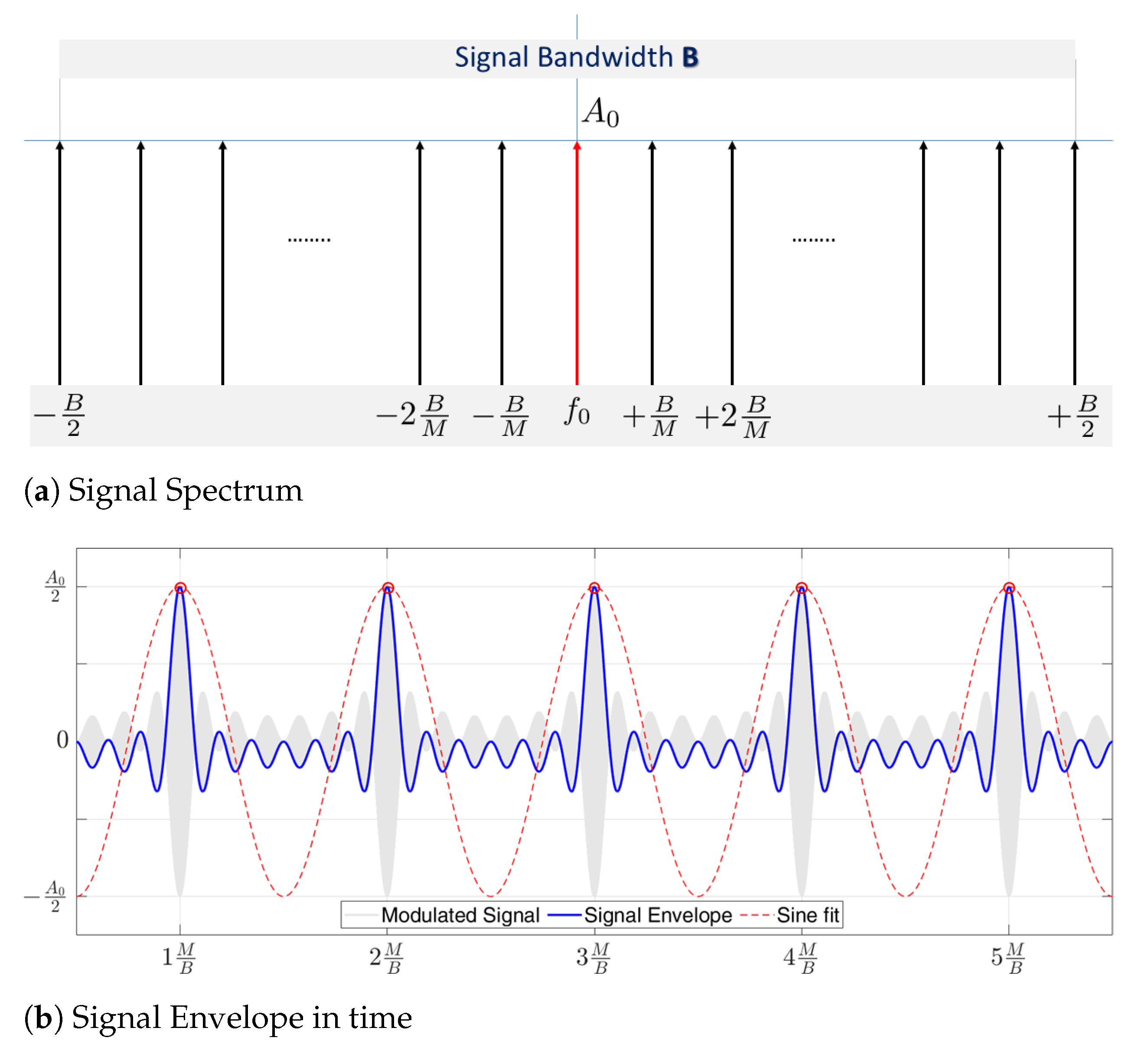
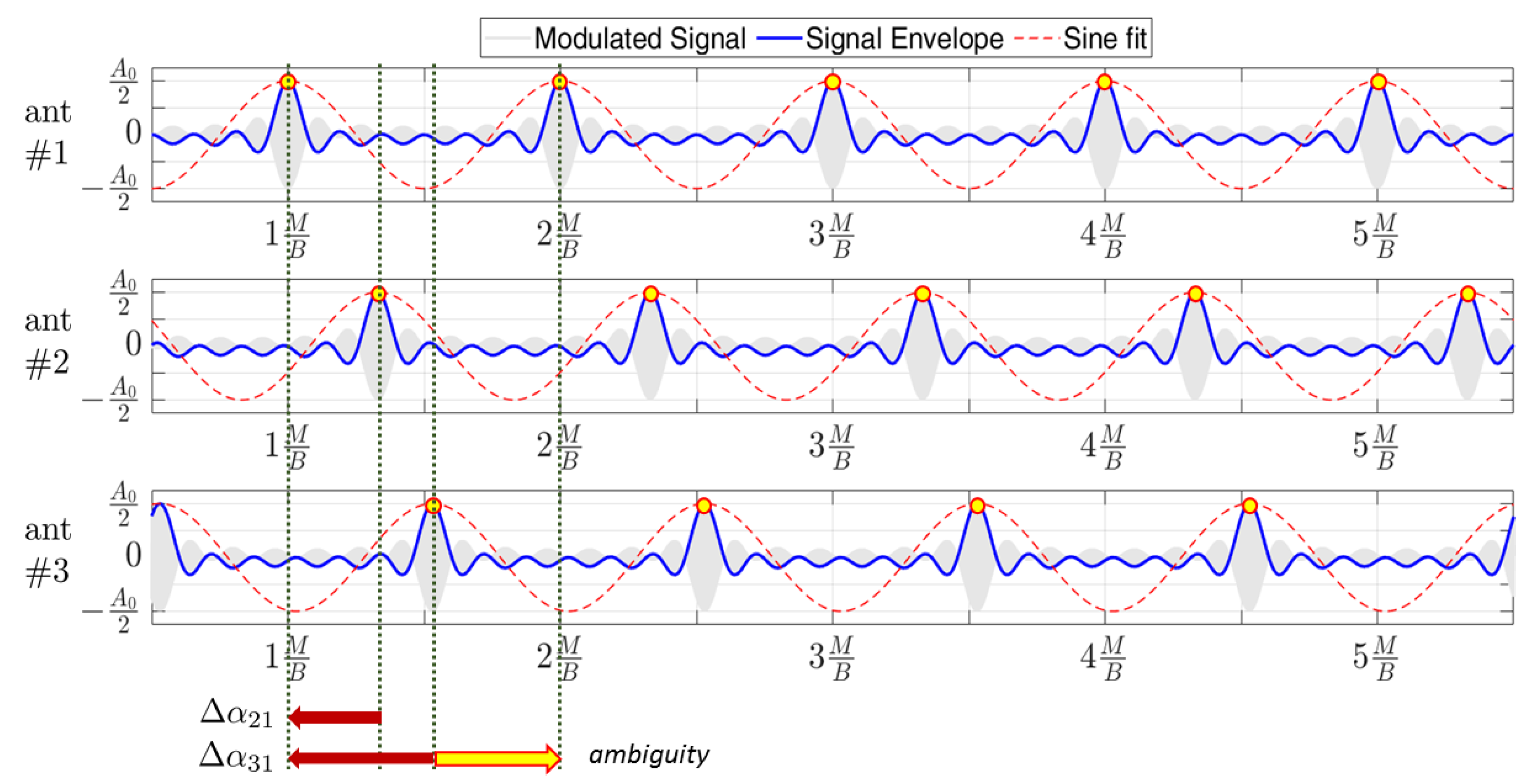
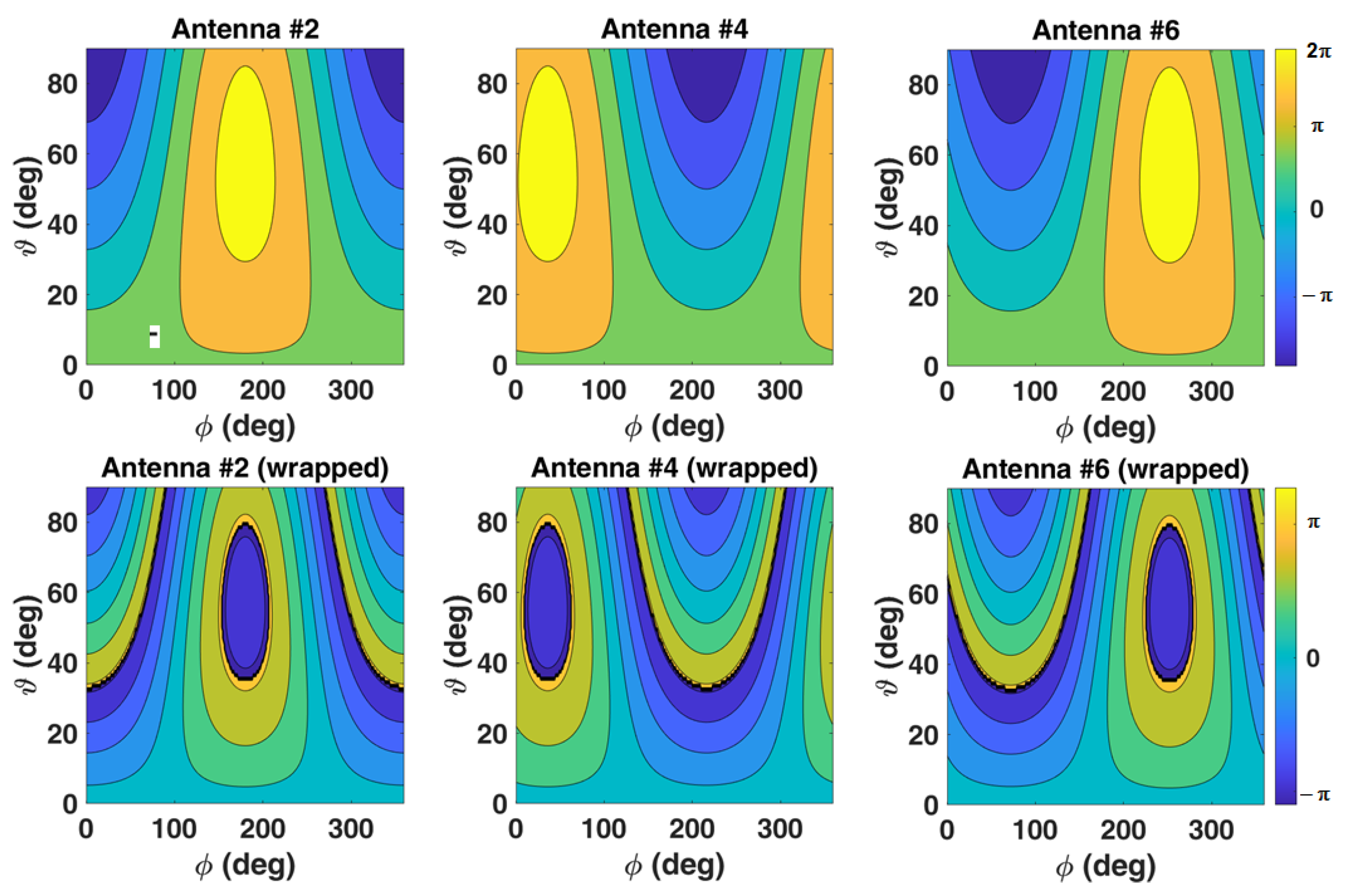
2.2. Phase-Wrapping Issues

Now, let us consider to implement a coherent sensing chain able to get complete amplitude-phase measurements for each term $s_i$ of (5). Dealing with a simple scenario as the one in Figure 1, it is trivial that it must result

$${\alpha }_5\le {\alpha }_4\le {\alpha }_3\le {\alpha }_1\le {\alpha }_2$$

(6)

where the sorting order is strictly dependent on signal direction of arrival $\left(\vartheta ,\phi \right)$. Note that such a sequence is preserved also applying a linear transform on each measured phase, so normalizing the steering vector respect to a generic R-th reference antenna as in (5) it results

$$\mathsf{\Delta }{\alpha }_{5R}\le \mathsf{\Delta }{\alpha }_{4R}\le \mathsf{\Delta }{\alpha }_{3R}\le \mathsf{\Delta }{\alpha }_{1R}\le \mathsf{\Delta }{\alpha }_{2R}\mathrm{with}\mathsf{\Delta }{\alpha }_{iR}=\left({\alpha }_i-{\alpha }_{\mathrm{R}}\right)$$

(7)

and the $\mathsf{\Delta }{\alpha }_{iR}$ terms are the ones depicted in (3).

Considering an ideal sensing chain the phase difference terms as defined in (3) is always monotone with respect to antenna distance. Unfortunately, a real phase detection is always impaired by phase wrapping issue, so measured $\mathsf{\Delta }{\alpha }_{iR}$ terms must be placed as

$$\mathsf{\Delta }{\widehat{\alpha }}_{iR}=\mathsf{\Delta }{\alpha }_{iR}mod2\pi =\left({\alpha }_i-{\alpha }_{\mathrm{R}}\right)mod2\pi$$

(8)

where the introduction of modulus operator (mod) has dramatic effects on phase information coherency, disrupting the phase terms sorting order as given in (7). To avoid such phenomena, a condition can be placed imposing that the maximum $\mathsf{\Delta }{\alpha }_{iR}$ term should be lower than $2\pi$. Because phase displacement terms are dependent on signal DoA, this would require to dynamically change the reference antenna considering an a priori knowledge of expected direction of arrival, which is nonsensical.

A more affordable condition could be the bounding of the maximum distance between center of phases of different antennas, so that given any reference antenna all terms of (7) will be surely lower than $2\pi$.

Considering (3), such condition can be written as

$$\max \left\{\overline{\mathbf{k}}\left(\vartheta ,\phi \right)·\left({\overline{\mathbf{r}}}_{\mathrm{j}}-{\overline{\mathbf{r}}}_{\mathrm{i}}\right)\right\}\le 2\pi \forall \mathrm{i}\in \left[1,N\right], \mathrm{j}\in \left[1,N\right], \left(\vartheta ,\phi \right)$$

(9)

and given an array structure it allows to identify a sub-domain for signal DoAs where the phase ambiguity is avoided (or rather, a “Field of View” similar to one defined by Nyquist sampling conditions for MIMO arrays [12,33,34]).

By array geometry, surely it can be put that

$$\overline{\mathbf{k}}\left(\vartheta ,\phi \right) · \left({\overline{\mathbf{r}}}_{\mathrm{j}}-{\overline{\mathbf{r}}}_{\mathrm{i}}\right)\le \left|\frac{2\pi }{{\lambda }_0}\right| · \underset{\mathrm{i},\mathrm{j}}{\max }\left|\mathsf{\Delta }{\overline{\mathbf{r}}}_{\mathrm{j}\mathrm{i}}\right|\le 2\pi \forall \mathrm{i}\in \left[1,N\right], \mathrm{j}\in \left[1,N\right], \left(\vartheta ,\phi \right)$$

(10)

so it results

$$\underset{\mathrm{i},\mathrm{j}}{\max }\left|\mathsf{\Delta }{\overline{\mathbf{r}}}_{\mathrm{j}\mathrm{i}}\right|\le {\lambda }_0\forall \mathrm{i}\in \left[1,N\right], \mathrm{j}\in \left[1,N\right]$$

(11)

and by (11) it is clear how much the dimensions of the entire array structure must be constrained in order to achieve an effective signal DoA estimation on the overall $\left(\vartheta ,\phi \right)$ domain.

As an example an array working in $f_0=2.45\mathrm{GHz}$, the IEEE 802.11bg WiFi frequency band should have the maximum distance between antennas center of phases equal to ${\lambda }_0=12.24\mathrm{cm}$, while shifting to the upper $f_0=5.2\mathrm{GHz}$ band for 802.11n such distance lowers to ${\lambda }_0=5.7\mathrm{cm}$. Dealing with a SBA system, as, for instance, the one described in Section 3, each antenna of the array will have physical dimensions comparable to ${\lambda }_0$, thus fulfilling such dimensional constraints will lead to serious device engineering issues.

2.3. Phase Reconstruction Method

The constraint on array structure dimensions is given by condition (11), which is a direct consequence of (3). A straight way to relax such condition is to increase the signal wavelength ${\lambda }_0$, but this would require to shift working frequency band.

This work aims to introduce a method able to unwrap actual phase detections by synthetically lowering the equivalent signal wavelength as placed in (3). For propagating single tone signals, the wavelength is given by [35]

$${\lambda }_0=\frac{v_{\mathrm{phase}}}{f_0}\mathrm{with}{v}_{\mathrm{phase}}=2\pi {\left|\frac{\overline{\mathbf{k}}}{f_0}\right|}^{-1},\left|\overline{\mathbf{k}}\right|=\frac{2\pi }{{\lambda }_0}=2\pi \left(\frac{f_0}{c_0}\right)\sqrt{{\epsilon }_R{\mu }_R}$$

(12)

where $v_{\mathrm{phase}}$ is the phase speed related to single tone propagation on propagation direction, $c_0$ is the speed of light, and ${\epsilon }_R,{\mu }_R$ are the relative dielectric and diamagnetic constants for propagation medium. Checking (12), it is clear that there is not any degree of freedom left for varying the equivalent ${\lambda }_0$ parameter.

Dealing with non-monochromatic signals, or rather modulated RF signals, the propagating speed of the entire signal envelope on propagating direction is no more equal to phase velocity but it equals the group velocity (13) [35].

$$v_{\mathrm{group}}=2\pi {\left({\left.\frac{\partial \left|\overline{\mathbf{k}}\right|}{\partial f}\right|}_{f=f_0}\right)}^{-1}\mathrm{with}\overline{\mathbf{k}}=f\left(A_{-\frac{M}{2}},f_{-\frac{M}{2}},\dots ,A_{\frac{M}{2}},f_{\frac{M}{2}}\right)\ne \frac{2\pi }{{\lambda }_0}$$

(13)

The group speed definition as given in (13) is too complex to be useful for inferring relation between modulating signal parameters and equivalent ${\lambda }_G$ obtained. Nevertheless, by (13) is clear how further degrees of freedom can be added by introducing a modulated signal in place of a single tone.

In place of a single-tone signal, consider using a multi-tone composed signal such as

$$s_{\mathrm{TX}}\left(t\right)=\left(\sum _{n=-\frac{M}{2}}^{\frac{M}{2}}{A}_n{e}^{j·2\pi ·n\mathsf{\Delta }f·t}\right)e^{j·2\pi ·f_0·t}\mathrm{with}\mathsf{\Delta }f=\frac{\mathrm{B}}{M}$$

(14)

where B is the pass-band signal bandwidth, M is the number of tones (even), and $A_i$ is the signal amplitude for the i-th tone. To simplify the scenario, (14) can be simplified considering a constant signal amplitude $A_i=A_0$ leading to signal in Figure 2a.

Figure 2 shows frequency and time domain plots for signal as defined by (14). Because the signal is composed by a discrete number of harmonics, its envelope is periodic with period and pulse width equal to

$$T_{\mathrm{period}}=\frac{1}{\mathsf{\Delta }f}=\frac{M}{\mathrm{B}},T_{\mathrm{pulse}}\approx \frac{1}{B}\mathrm{with}M<\mathrm{B}$$

(15)

It is possible to exploit signal periodicity trying to fit a simpler signal model on transmitted signal. For instance in Figure 2b a monochromatic signal coarsely fits on actual signal, preserving the matching simply the signal maximums to envelope maximums. The fit signal model can be written as

$$s_{\mathrm{FIT}}\left(t,{\beta }_{\mathrm{FIT}}\right)=A_0{e}^{j\left(2\pi f_{\mathrm{FIT}}t-{\beta }_{\mathrm{FIT}}\right)}$$

(16)

where $f_{\mathrm{FIT}}$ and ${\beta }_{\mathrm{FIT}}$ are chosen to achieve the hard matching between real signal and fit signal maximums. Note that $f_{\mathrm{FIT}}$ is known by reference signal periodicity and it results

$$f_{\mathrm{FIT}}=\frac{1}{T_{\mathrm{period}}}=\frac{\mathrm{B}}{M}$$

(17)

while ${\beta }_{\mathrm{FIT}}$ provides the exact alignment of maximums by shifting the fit signal.

Until now, the proposed signal model has been fit considering a specific starting time for the signal envelope, thus providing a fixed value for ${\beta }_{\mathrm{FIT}}$. Nevertheless, we are dealing with a propagating signal, so changing the observation point we expect to observe a time shift on signal observations in Figure 2b.

Similarly to (1), in the fit signal model the starting phase shift due to changing of observation point can be put as

$${\beta }_{\mathrm{FIT}}={\overline{\mathbf{k}}}_{\mathrm{FIT}}\left(\vartheta ,\phi \right) · \left(\overline{\mathbf{r}}-{\overline{\mathbf{r}}}_0\right)$$

(18)

where ${\overline{\mathbf{r}}}_0$ is the initial observation point, $\overline{\mathbf{r}}$ the new one, and ${\overline{\mathbf{k}}}_{\mathrm{FIT}}$ the wave vector describing the equivalent fit signal propagation. Note that the latter can be defined as

$${\overline{\mathbf{k}}}_{\mathrm{FIT}}=\left(\frac{2\pi }{{\lambda }_{\mathrm{FIT}}}\right)\widehat{\mathbf{k}}=2\pi \left(\frac{f_{\mathrm{FIT}}}{v_{\mathrm{group}}}\right)\widehat{\mathbf{k}}=2\pi \left(\frac{\mathrm{B}}{M·v_{\mathrm{group}}}\right)\widehat{\mathbf{k}}$$

(19)

where the $v_{\mathrm{group}}$ parameter is still unknown. Despite this, Equation (1) can be rewritten as a typical single-tone propagating wave impinging on the i-th antennas of an array

$$s_{\mathrm{FIT}}\left(t,\mathrm{i}\right)=A_0{e}^{j\left(2\pi \frac{\mathrm{B}}{M}t-{\overline{\mathbf{k}}}_{\mathrm{FIT}}\left(\vartheta ,\phi \right)·{\overline{\mathbf{r}}}_{\mathrm{i}}\right)}$$

(20)

where, exactly as in (1), ${\overline{\mathbf{r}}}_{\mathrm{i}}$ is the i-th antenna center of phase position vector with respect to reference system $\overline{\mathbf{O}}$, as indicated in Figure 1.

Because the model in (20) exactly resembles the fundamental propagation model, to avoid the phase-wrapping issue the condition in (10), it can be put again that

$$\underset{\mathrm{i},\mathrm{j}}{\max }\left|\mathsf{\Delta }{\overline{\mathbf{r}}}_{\mathrm{j}\mathrm{i}}\right|\le {\lambda }_{\mathrm{FIT}}\forall \mathrm{i}\in \left[1,N\right], \mathrm{j}\in \left[1,N\right]$$

(21)

but observing Figure 2b it is clear that ${\lambda }_{\mathrm{FIT}}>>{\lambda }_0$. Following (19), the equivalent wavelength for signal fit can be written as

$${\lambda }_{\mathrm{FIT}}=\frac{M·v_{\mathrm{group}}}{\mathrm{B}}$$

(22)

so theoretically the condition in (21) can be relaxed considering a multi-tone transmitted signal as defined in (14), optimizing the number of tones M and the bandwidth B. Relaxing condition (22) straightly enables to recover phase-information on phase-impaired scenario as in Figure 1. A pictorial proof of such concept is shown in Figure 3.

In Figure 3, three hypothetical impinging signal traces, with transmitted signal defined as in (1), are depicted. As in Figure 2b, the wavelength for $f_0$ frequency is too small respect to the signal period; in fact, it is not possible to get a meaningful phase difference value considering the RF signal carrier. Conversely, the maximum distance between signal peaks is large, making possible to define a unambiguous phase delay $\mathsf{\Delta }{\alpha }_{21},\mathsf{\Delta }{\alpha }_{31}$ also for higher time delays, or higher distances between different antennas. As a drawback dealing with periodic signals still leaves a risk of ambiguity, and in next Section such point will be discussed.

By a practical standpoint it means that the receiver chain should sample the received signal envelope depicted in Figure 2, and a postprocessing unit has to extract signal features in order to get peak amplitude $A_i$, proportional to each antenna gain $G_i\left(\vartheta ,\phi \right)$, and relative phase ${\beta }_{\mathrm{FIT}}$ parameters related in some way to received signal relative time shiftings (Figure 3). The right time shifting information is preserved only if the antenna switching mechanism is synchronized to the transmitted signal period, to ensure the coherency of time domains between different acquisitions.

Considering Figure 3, it is conceptually clear that doing feature estimations on different antenna signals and embedding these information in a steering vector, the latter shall contain an overall phase displacement information not impaired by wrapping. By this, a generic DoA estimation algorithm can be involved without any kind of issue.

Note that in (22) the $v_{\mathrm{group}}$ is still undetermined, and despite a generic definition of such term is given in (13), achieving an analytical formula for ${\lambda }_{\mathrm{FIT}}$ could be a challenging task. In the following, a computational way to get the ${\lambda }_{\mathrm{FIT}}$ and the ${\overline{\mathbf{k}}}_{\mathrm{FIT}}$ terms is given.

Consider that to have an ideal coherent IQ receiver connected through a switch to each different antenna of the array, as in Figure 4. For either I and Q demodulator output channels, the signal is sampled fulfilling the Nyquist sampling condition for signal given in (14) providing $f_{\mathrm{SAMPLE}}\ge \mathrm{B}$, with bandwidth B defined as in Figure 2. The antenna switching mechanism is synchronized to signal period $T_{\mathrm{period}}$ to ensure time domain coherency between different antenna readings.

Given a transmitted signal $s_{\mathrm{TX}}\left(t\right)=s\left(t\right)$, an ideal radio-link of distance R would provide a received signal equal to

$$s_{\mathrm{RX}}\left(t\right)=G_R{H}_0{s}_{\mathrm{TX}}\left(t-\tau \right)\mathrm{with}\tau =\frac{R}{c_0}$$

(23)

where $\tau$ corresponds to the propagation delay, $G_R$ the receiver antenna gain, and $H_0$ the coefficient modeling transmission gain and radio link path-loss, as the effects of the radio channel. Applying concepts of dynamic system modeling, it can also be written that

$$s_{\mathrm{RX}}\left(t\right)=s_{\mathrm{TX}}\left(t\right) \otimes h\left(t\right)\iff S_{\mathrm{RX}}\left(f\right)=S_{\mathrm{TX}}\left(f\right)·H\left(f\right)$$

(24)

where $H\left(f\right)$ is the radio channel transfer function with related impulsive response $h\left(t\right)$. Considering a wide-band signal, the path-loss cannot be defined by a single value, so the channel transfer function must be written as

$$H\left(f\right)=\left|H\left(f\right)\right|·e^{j\angle H\left(f\right)}\mathrm{with}\left\{\begin{array}{c}\left|H\left(f\right)\right|=G_R{G}_T{\left(\frac{c_0}{f}\frac{1}{4\pi R}\right)}^2\hfill \\ \angle H\left(f\right)=-2\pi ·f·\tau +{\gamma }_0\hfill \end{array}\right.$$

(25)

in the case of broadband transmitting and receiving antennas with constant gains $G_T$ and $G_R$ along the entire signal bandwidth, and a generic phase misalignment ${\gamma }_0$ between $f_0$ receiver local oscillator and transmitter one [36]. Factorizing the variation term on signal components frequencies with respect to the transform function reference value in the carrier frequency $f_0$, the transfer function can be rewritten as

$$H\left(f\right)=G_R{H}_0·H_{\mathsf{\Delta }}\left(f\right)\mathrm{with}\left\{\begin{array}{c}{H}_0=G_T{\left(\frac{c_0}{f_0}\frac{1}{4\pi R}\right)}^2{e}^{j{\gamma }_0}\hfill \\ H_{\mathsf{\Delta }}\left(f\right)={\left(\frac{f_0}{f}\right)}^2{e}^{-j·2\pi ·f·\tau }\hfill \end{array}\right.$$

(26)

The postprocessing unit in Figure 4 is able to get a complete time observation of complex envelope signal as in Figure 2, because IQ demodulation provides the frequency shifting of bandpass signal centered in $f_0$ to baseband keeping spectrum asymmetries and relative tone phases. The base-band converted IQ digital signal equals to

$${s_{\mathrm{BB}}}_{\mathrm{RX}}\left(t\right)=s_{\mathrm{RX}}\left(t\right)·e^{-j·2\pi ·f_0·t}=G_R{H}_0{e}^{-j·2\pi ·f_0·\tau }\sum _{n=-\frac{M}{2}}^{\frac{M}{2}}{A}_n{e}^{j·2\pi ·n\frac{\mathrm{B}}{M}·\left(t-\tau \right)}$$

(27)

where the $f_0$ frequency related term is removed due to base-band conversion. The resulting Fourier transform for base-band signal is

$${S_{\mathrm{BB}}}_{\mathrm{RX}}\left(f\right)=S_{\mathrm{RX}}\left(f+f_0\right)$$

(28)

so its spectrum is exactly the one depicted in Figure 2, shifted to a center frequency $f_0=0$ Hz.

To deal with variation in path-loss, a slight modification in transmitted signal must be taken in account to equalize signal alteration due to propagation. Practically, the transmitted signal spectrum is changed to

$$S_{\mathrm{TX}}\left(f\right)=A_{\mathrm{TX}}·{\left(\frac{f}{f_0}\right)}^2\mathrm{with}f\in \left[f_0-\frac{B}{2},f_0+\frac{B}{2}\right]$$

(29)

and this allows to get the received signal

$$S_{\mathrm{RX}}\left(f\right)=S_{\mathrm{TX}}\left(f\right)·H\left(f\right)=A_{\mathrm{TX}}{G}_R{H}_0{e}^{-j·2\pi ·f·\tau }$$

(30)

Let consider again a multi-antenna structure as the one in Figure 1, with the objective of identifying a steering vector as in (5). The Antenna Switch state is changed by the uC after getting enough samples for each antenna. This leads to get different signal streams ${s_{\mathrm{BB}}}_{\mathrm{RX}}\left(t,\mathrm{i}\right)$, one for each antenna, as

$${s_{\mathrm{BB}}}_{\mathrm{RX}}\left(t,\mathrm{i}\right)=G_i\left(\vartheta ,\phi \right)·H_0{e}^{-j·2\pi ·f_0·{\tau }_{\mathrm{i}}}\sum _{n=-\frac{M}{2}}^{\frac{M}{2}}{A}_n{e}^{j·2\pi ·n\frac{\mathrm{B}}{M}·\left(t-{\tau }_{\mathrm{i}}\right)}$$

(31)

where the delay ${\tau }_{\mathrm{i}}$ and the $G_i\left(\vartheta ,\phi \right)$ antenna gain coefficients take in account the radio-link variations due to the swapping of receiving antenna. The antenna array is not distributed (Figure 1) thus for every antenna the radio-link distance R is considered to be the same thus $H_0$ is not dependent on antenna index. Note that the Local Oscillator phase misalignment term ${\gamma }_0$ is supposed to be the same between all the antennas, and this condition can be satisfied implementing a PLL to get the phase-lock with equal phase offset on the $f_0$ carrier signal.

In order to define a steering vector as in (5) a single amplitude-phase coefficient for the equivalent wavelength signal must be produced by each different antenna signal observation. Consider applying the condition on monochromatic signal fit as proposed in Figure 2, imposing equivalence between equivalent and received signals peaks, given that all the different antenna readings share the same time reference as specified in Figure 4.

Assuming a monochromatic signal propagation the i-th steering vector term is

$$s_{\mathrm{i}}=A_{\mathrm{FIT}}{G}_{\mathrm{i}}\left(\vartheta ,\phi \right)H_0{e}^{-j{\beta }_{\mathrm{FIT}}}\mathrm{with}{\beta }_{\mathrm{FIT}}={\overline{\mathbf{k}}}_{\mathrm{FIT}}\left(\vartheta ,\phi \right)·{\overline{\mathbf{r}}}_{\mathrm{i}}$$

(32)

and taking in account that the equivalent signal must have the same peak as the real one it must be

$$A_{\mathrm{FIT}}={\int }_{-\frac{\mathrm{B}}{2}}^{\frac{\mathrm{B}}{2}}{A}_{\mathrm{TX}}\mathrm{d}f=A_{\mathrm{TX}}·\mathrm{B}.$$

(33)

The normalized term respect the R-th reference antenna results in

$$s_{\mathrm{i}\mathrm{R}}=\frac{G_{\mathrm{i}}\left(\vartheta ,\phi \right)}{G_{\mathrm{R}}\left(\vartheta ,\phi \right)}{e}^{-j{\overline{\mathbf{k}}}_{\mathrm{FIT}}\left(\vartheta ,\phi \right)·\left({\overline{\mathbf{r}}}_{\mathrm{i}}-{\overline{\mathbf{r}}}_{\mathrm{R}}\right)}.$$

(34)

Because the steering vector term is the complex coefficient which models phase shift and amplitude gain given by the i-th antenna reception on signal, considering the baseband signal observations it results that

$$s_{\mathrm{FIT}}\left(t, \mathsf{i}\right)=s_{\mathrm{i}}·e^{j\left(2\pi f_{\mathrm{FIT}}t\right)}\mathrm{with}{f}_{\mathrm{FIT}}=\frac{\mathrm{B}}{M}=\frac{1}{T_{\mathrm{period}}}$$

(35)

thus the imposition of peaks equivalence is placed as

$$s_{\mathrm{FIT}}\left({{\tau }_{\mathrm{PK}}}_{\mathrm{i}}, \mathsf{i}\right)={s_{\mathrm{BB}}}_{\mathrm{RX}}\left({{\tau }_{\mathrm{PK}}}_{\mathrm{i}},\mathrm{i}\right)$$

(36)

where ${{\tau }_{\mathrm{PK}}}_i$ is known by signal observations. Merging (35) with (36) it results that

$$s_i={s_{\mathrm{BB}}}_{\mathrm{RX}}\left({{\tau }_{\mathrm{PK}}}_{\mathrm{i}},\mathrm{i}\right)e^{-j\left(2\pi \frac{{{\tau }_{\mathrm{PK}}}_{\mathrm{i}}}{T_{\mathrm{period}}}\right)}$$

(37)

so the $s_i$ terms can be extracted by features measurements of received ${s_{\mathrm{BB}}}_{\mathrm{RX}}\left(t,i\right)$ signals, each one evaluated in the peak instant time ${{\tau }_{\mathrm{PK}}}_{\mathrm{i}}$.

As indicated in Section 2.1, all steering vector terms can be normalized respect the same coefficient. Considering a generic R-th reference antenna, each term $s_i$ can be rewritten as

$$s_{i\mathrm{R}}=\frac{s_i}{s_{\mathrm{R}}}=\frac{{s_{\mathrm{BB}}}_{\mathrm{RX}}\left({{\tau }_{\mathrm{PK}}}_{\mathrm{i}},\mathrm{i}\right)}{{s_{\mathrm{BB}}}_{\mathrm{RX}}\left({{\tau }_{\mathrm{PK}}}_{\mathrm{R}},\mathrm{R}\right)}{e}^{-j\left[2\pi \frac{\left({{\tau }_{\mathrm{PK}}}_{\mathrm{i}}-{{\tau }_{\mathrm{PK}}}_{\mathrm{R}}\right)}{T_{\mathrm{period}}}\right]}$$

(38)

and the latter shows the measurement formula for each antenna of the array.

Note that the phase term could lead to phase-wrapping issues and its presence is related to ambiguity given by signal periodicity (Figure 3). To avoid such drawback a further condition can be put on exponential argument in (38). In fact, if it is placed

$$\underset{\mathrm{i},\mathrm{j}\in \left[1,N\right]}{\max }\frac{\left|{{\tau }_{\mathrm{PK}}}_{\mathrm{i}}-{{\tau }_{\mathrm{PK}}}_{\mathrm{R}}\right|}{T_{\mathrm{period}}}\le 1$$

(39)

the exponential term can be neglected avoiding any phase-wrapping issue. In addition to this it must be assured that the sample time $T_{\mathrm{sample}}$ is lower than minimum delay between different antennas to be sure that every antenna will measure a different peak arrival time. Considering the maximum signal propagation speed of $c_0$, the equation above can be placed with respect to distance between antenna center of phases

$$\left\{\begin{array}{c}{T}_{\mathrm{period}}=\frac{M}{\mathrm{B}}\ge \underset{\mathrm{i},\mathrm{j}\in \left[1,N\right]}{\max }\frac{\left|\mathsf{\Delta }{\overline{\mathbf{r}}}_{\mathrm{j}\mathrm{i}}\right|}{c_0}\hfill \\ T_{\mathrm{sample}}=\frac{1}{\mathrm{B}}\le \underset{\mathrm{i},\mathrm{j}\in \left[1,N\right]}{\max }\frac{\left|\mathsf{\Delta }{\overline{\mathbf{r}}}_{\mathrm{j}\mathrm{i}}\right|}{c_0}\hfill \end{array}\right.$$

(40)

and when the latter equations are satisfied the steering vector obtained as in (38) will present consistent phase information.

Note that while the conditions above enable to get a phase consistent steering vector, the analytical form for ${\overline{\mathbf{k}}}_{\mathrm{FIT}}\left(\vartheta ,\phi \right)$ as in (19) is still undetermined due to lack of knowledge about the $v_{\mathrm{group}}$ term.

2.4. Definition of a Valid Observation Model

As summarized in Section 2.1, a valid observation model is needed to calculate the ideal expected steering vectors belonging to the reference map [16,22,24]. Such a model must be entirely defined, as in (4) the reference map $\mathbf{M}\left(\vartheta ,\phi \right)$ shall be defined as a function of DoA domain only. The easiest way to define the latter is to implement the definition for the $s_i$ terms as given in (32).

Let consider the expected physical steering-vector related to RF signal propagation. Considering the relationship between the baseband signal and the RF signal it results that

$$s_{i\mathrm{R}}=\frac{s_{\mathrm{RX}}\left({{\tau }_{\widetilde{\mathrm{PK}}}}_{\mathrm{i}},\mathrm{i}\right)e^{-j2\pi f_0{{\tau }_{\widetilde{\mathrm{PK}}}}_{\mathrm{i}}}}{s_{\mathrm{RX}}\left({{\tau }_{\widetilde{\mathrm{PK}}}}_{\mathrm{R}},\mathrm{R}\right)e^{-j2\pi f_0{{\tau }_{\widetilde{\mathrm{PK}}}}_{\mathrm{R}}}}$$

(41)

where ${{\tau }_{\widetilde{\mathrm{PK}}}}_{\mathrm{i}}$ is the real peak delay respect the beginning of signal transmission. Until now, the ${{\tau }_{\mathrm{PK}}}_{\mathrm{i}}$ terms have been defined as the time instant associated to the i-th received signal peak within the baseband observation window.

The real received peak time ${{\tau }_{\widetilde{\mathrm{PK}}}}_{\mathrm{i}}$ is related to measured ${{\tau }_{\mathrm{PK}}}_{\mathrm{i}}$ as

$${{\tau }_{\mathrm{PK}}}_{\mathrm{i}}={{\tau }_{\widetilde{\mathrm{PK}}}}_{\mathrm{i}}-{t_0}_{\mathrm{i}}\forall \mathrm{i}\in \left[1,N\right]$$

(42)

where ${t_0}_{\mathrm{i}}$ is the time offset between the transmission and the beginning of signal period observation. Despite such offset is unknown if the period synchronization between different antenna time windows is ensured (Figure 4) we can suppose that ${t_0}_{\mathrm{i}}=t_0$ is constant for the entire set of readings. By this the difference between measured time peaks result

$${{\tau }_{\mathrm{PK}}}_{\mathrm{i}}-{{\tau }_{\mathrm{PK}}}_{\mathrm{j}}={{\tau }_{\widetilde{\mathrm{PK}}}}_{\mathrm{i}}-{{\tau }_{\widetilde{\mathrm{PK}}}}_{\mathrm{j}}\forall \mathrm{i},\mathrm{j}\in \left[1,N\right].$$

(43)

Considering the transmitted signal spectrum as in (29) and the transfer function as in (26) it results

$$\begin{array}{cc}\hfill s_{\mathrm{RX}}({{\tau }_{\widetilde{\mathrm{PK}}}}_{\mathrm{i}},\mathrm{i})e^{-j2\pi f_0{{\tau }_{\widetilde{\mathrm{PK}}}}_{\mathrm{i}}}& ={\int }_{f_0-\frac{\mathrm{B}}{2}}^{f_0+\frac{\mathrm{B}}{2}}{S}_{\mathrm{TX}}\left(f\right)H\left(f\right)e^{j2\pi \left(f-f_0\right){{\tau }_{\widetilde{\mathrm{PK}}}}_{\mathrm{i}}}\mathrm{d}f\hfill \\ \hfill & =A_{\mathrm{TX}}{G}_i\left(\vartheta ,\phi \right)H_0{\int }_{f_0-\frac{\mathrm{B}}{2}}^{f_0+\frac{\mathrm{B}}{2}}{e}^{-j·2\pi ·f·{\tau }_{\mathrm{i}}}{e}^{j2\pi \left(f-f_0\right){{\tau }_{\widetilde{\mathrm{PK}}}}_{\mathrm{i}}}\mathrm{d}f\hfill \\ \hfill & =A_{\mathrm{TX}}{G}_i\left(\vartheta ,\phi \right)H_0{e}^{-j2\pi f_0{{\tau }_{\widetilde{\mathrm{PK}}}}_{\mathrm{i}}}{\int }_{f_0-\frac{\mathrm{B}}{2}}^{f_0+\frac{\mathrm{B}}{2}}{e}^{j2\pi f\left({{\tau }_{\widetilde{\mathrm{PK}}}}_{\mathrm{i}}-{\tau }_{\mathrm{i}}\right)}\mathrm{d}f\hfill \\ \hfill & =\left(A_{\mathrm{TX}}\mathrm{B}{H}_0\right)G_i\left(\vartheta ,\phi \right)sinc(\mathrm{B}·({{\tau }_{\widetilde{\mathrm{PK}}}}_{\mathrm{i}}-{\tau }_i))e^{-j2\pi f_0{{\tau }_{\widetilde{\mathrm{PK}}}}_{\mathrm{i}}}\hfill \end{array}$$

(44)

so (41) becomes

$$s_{i\mathrm{R}}=\frac{G_i\left(\vartheta ,\phi \right)}{G_R\left(\vartheta ,\phi \right)}·\frac{sinc(\mathrm{B}·({{\tau }_{\widetilde{\mathrm{PK}}}}_{\mathrm{i}}-{\tau }_i))}{sinc(\mathrm{B}·({{\tau }_{\widetilde{\mathrm{PK}}}}_{\mathrm{R}}-{\tau }_{\mathrm{R}}))}·e^{-j2\pi f_0\left({{\tau }_{\mathrm{PK}}}_{\mathrm{i}}-{{\tau }_{\mathrm{PK}}}_{\mathrm{j}}\right)}.$$

(45)

Considering that for each antenna the shape of transmitted pulse is the same it results that

$${{\tau }_{\widetilde{\mathrm{PK}}}}_{\mathrm{i}}-{\tau }_{\mathrm{i}}={{\tau }_{\widetilde{\mathrm{PK}}}}_{\mathrm{j}}-{\tau }_{\mathrm{j}}\forall \mathrm{i}, \mathrm{j}$$

(46)

so finally we get

$$s_{i\mathrm{R}}=\frac{G_i\left(\vartheta ,\phi \right)}{G_R\left(\vartheta ,\phi \right)}·e^{-j2\pi f_0\left({{\tau }_{\mathrm{PK}}}_{\mathrm{i}}-{{\tau }_{\mathrm{PK}}}_{\mathrm{R}}\right)}$$

(47)

and the steering vector term defined as this has exactly the same form as given in (5) for the propagation of a monochromatic signal. The signal fit is defined as monochromatic, so let force the signal propagation speed to $c_0$, putting

$${{\tau }_{\mathrm{PK}}}_{\mathrm{i}}-{{\tau }_{\mathrm{PK}}}_{\mathrm{j}}=\frac{\widehat{\mathbf{k}}\left(\vartheta ,\phi \right)·\mathsf{\Delta }{\overline{\mathbf{r}}}_{\mathrm{j}\mathrm{i}}}{c_0}$$

(48)

Forcing the equivalence between (47) and the signal fit steering vector in (34) results in

$$e^{-j{\overline{\mathbf{k}}}_{\mathrm{FIT}}\left(\vartheta ,\phi \right)·\left({\overline{\mathbf{r}}}_{\mathrm{i}}-{\overline{\mathbf{r}}}_{\mathrm{R}}\right)}=e^{-j2\pi f_0\frac{\widehat{\mathbf{k}}\left(\vartheta ,\phi \right)·\left({\overline{\mathbf{r}}}_{\mathrm{i}}-{\overline{\mathbf{r}}}_{\mathrm{R}}\right)}{c_0}}$$

(49)

thus the phase equivalence condition is

$$\left[{\overline{\mathbf{k}}}_{\mathrm{FIT}}\left(\vartheta ,\phi \right)·\left({\overline{\mathbf{r}}}_{\mathrm{i}}-{\overline{\mathbf{r}}}_{\mathrm{R}}\right)\right]mod2\pi =\left[2\pi f_0\frac{\widehat{\mathbf{k}}\left(\vartheta ,\phi \right)·\left({\overline{\mathbf{r}}}_{\mathrm{i}}-{\overline{\mathbf{r}}}_{\mathrm{R}}\right)}{c_0}\right]mod2\pi .$$

(50)

The second term of (49) surely shows phase wrapping if the array is not rightly scaled considering the $f_0$ wavelength, as described in Section 2.2.

The first term argument is the phase term related to baseband fit signal as put in Section 2.3. If conditions on transmitting signal in (40) are fulfilled, it is given that such term will not show any phase-wrapping issue thus (50) becomes

$${\overline{\mathbf{k}}}_{\mathrm{FIT}}\left(\vartheta ,\phi \right)·\left({\overline{\mathbf{r}}}_{\mathrm{i}}-{\overline{\mathbf{r}}}_{\mathrm{R}}\right)=\left[2\pi f_0\frac{\widehat{\mathbf{k}}\left(\vartheta ,\phi \right)·\left({\overline{\mathbf{r}}}_{\mathrm{i}}-{\overline{\mathbf{r}}}_{\mathrm{R}}\right)}{c_0}\right]mod2\pi$$

(51)

and merging with (19) it results that

$$v_{\mathrm{group}}\left(\vartheta ,\phi ,\mathrm{i}\right)=2\pi \left(\frac{\mathrm{B}}{M}\right)\frac{\left|{\overline{\mathbf{r}}}_{\mathrm{i}}-{\overline{\mathbf{r}}}_{\mathrm{R}}\right|}{\left[2\pi f_0\frac{\widehat{\mathbf{k}}\left(\vartheta ,\phi \right)·\left({\overline{\mathbf{r}}}_{\mathrm{i}}-{\overline{\mathbf{r}}}_{\mathrm{R}}\right)}{c_0}\right]mod2\pi }·cos\mathsf{\Delta }\alpha$$

(52)

with

$$cos\mathsf{\Delta }\alpha =\widehat{\mathbf{k}}\left(\vartheta ,\phi \right)·\left(\frac{{\overline{\mathbf{r}}}_{\mathrm{i}}-{\overline{\mathbf{r}}}_{\mathrm{R}}}{\left|{\overline{\mathbf{r}}}_{\mathrm{i}}-{\overline{\mathbf{r}}}_{\mathrm{R}}\right|}\right)$$

(53)

and consequently

$${\lambda }_{\mathrm{FIT}}\left(\vartheta ,\phi ,\mathrm{i}\right)=2\pi \frac{\widehat{\mathbf{k}}\left(\vartheta ,\phi \right)·\left({\overline{\mathbf{r}}}_{\mathrm{i}}-{\overline{\mathbf{r}}}_{\mathrm{R}}\right)}{\left[2\pi f_0\frac{\widehat{\mathbf{k}}\left(\vartheta ,\phi \right)·\left({\overline{\mathbf{r}}}_{\mathrm{i}}-{\overline{\mathbf{r}}}_{\mathrm{R}}\right)}{c_0}\right]mod2\pi }.$$

(54)

Note that following this, the $v_{\mathrm{group}}\left(\vartheta ,\phi \right)$ and ${\lambda }_{\mathrm{FIT}}\left(\vartheta ,\phi \right)$ functions have no more actual physical meaning, even resulting different between different antennas. They become terms needed to build an equivalent model able to describe the expected phase displacement among the array elements. Anyway, now the equivalent wave vector is defined through a deterministic function of the DoA domain which leads to expected evaluations consistent with measurements; thus, the latter can be used to build an effective reference map $\mathbf{M}\left(\vartheta ,\phi \right)$ as required in (4).

3. TDoA Method Experimental Validation

This section describes a possible hardware suitable for the implementation for the methodology introduced above. To prove the method effectiveness, a massive campaign of DoA estimations was carried out by means of a phase-impaired anchor device based on a SBA array. Thus, Cumulative Density Functions (CDFs) of DoAs estimation errors, with and without the use of phase reconstruction, are compared to assess the improvements given by the proposed solution.

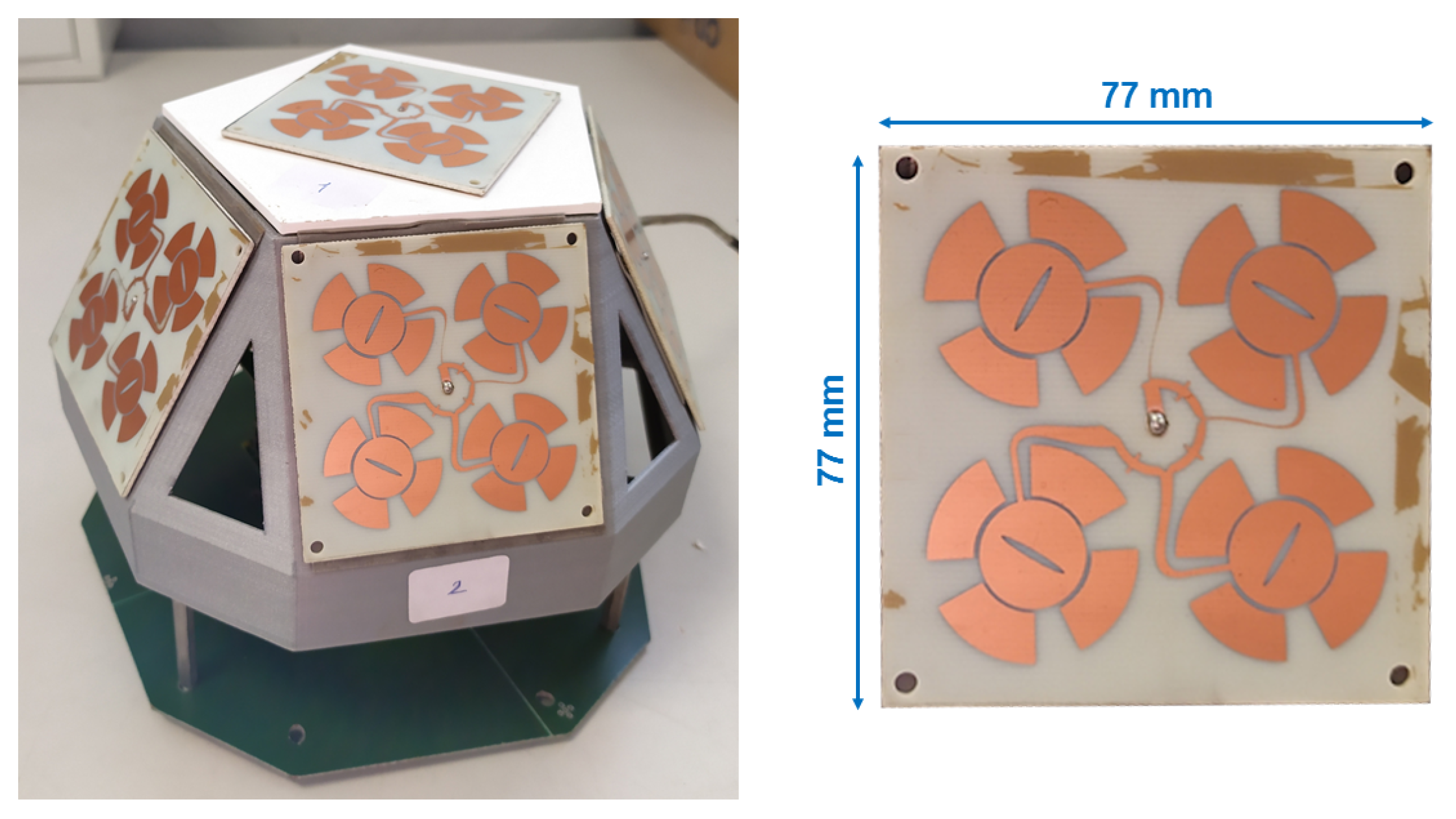
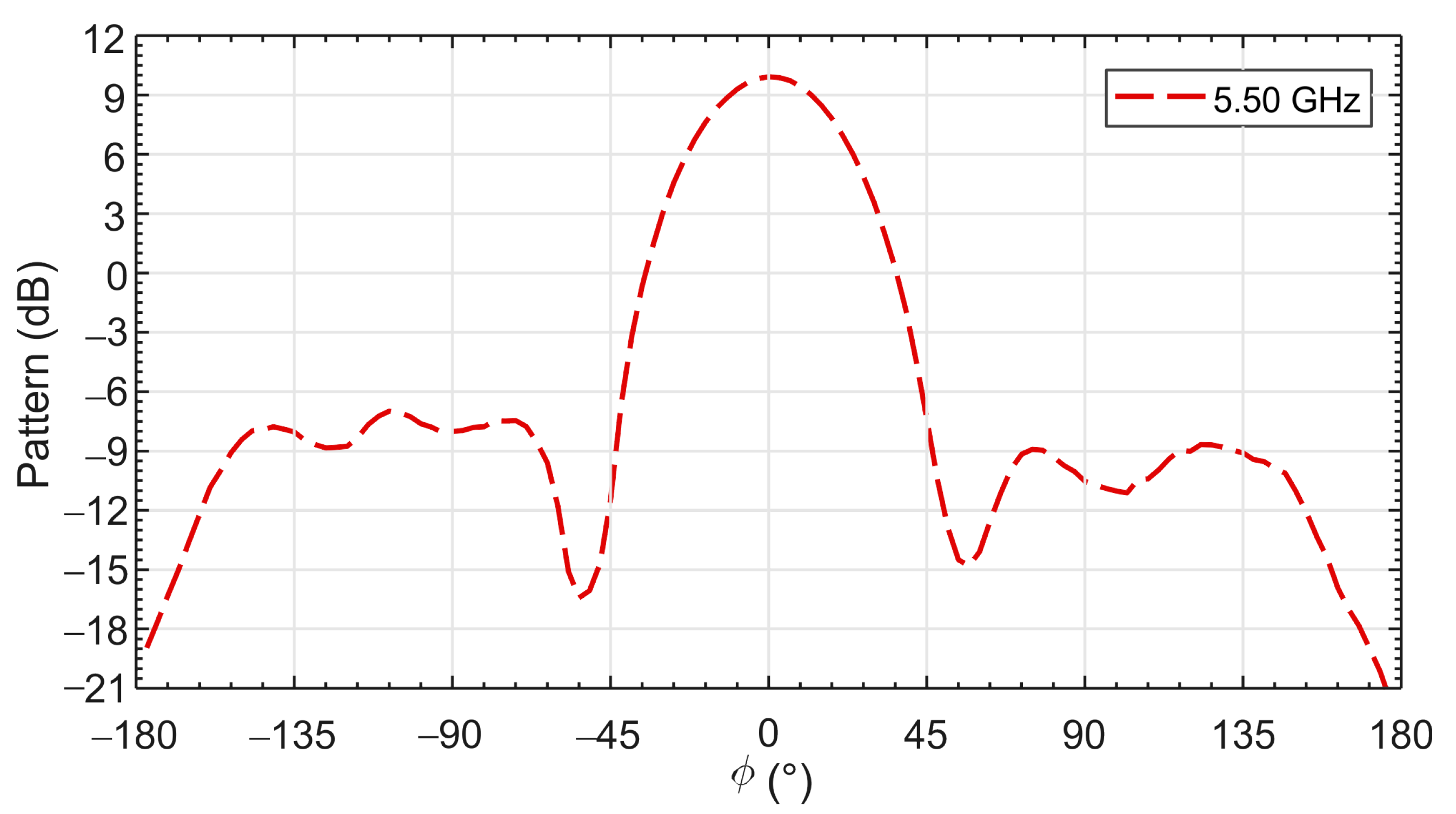
3.1. Anchor Switched Beam Antenna Design

The SBA-based anchor device is capable to enable the Space Division Multiplexing Access (SDMA) approach, whose structure is shown in Figure 5. The structure is engineered to be well suited for DoA estimations for phase-less observations, ensuring a complete coverage of hemispherical domain surrounding to the device, according to [37,38].

The six antennas that compose the anchor system are designed to operate in the nominal bandwidth 4–7 GHz. The individual antenna element that composes the SBA, is a 2 × 2 array of patch antennas, whose design was proposed in [39,40]. They are and arranged to cover a semi-spherical range, following the design technique proposed in [41].

Each antenna element works in circular polarization (CP), increasing the robustness of the radio link and thus contrasting the multi-path impairment, regardless of the relative orientation of the target. In Figure 6, the radiation pattern of the six patch antennas implemented in the SBA at the center frequency of 5.5 GHz is reported; for the purpose of the localization purpose, these can be considered to be identical. The Half-Power Beamwidth is reasonably maintained constant across the entire working frequency band. A detailed antenna performance is provided in

Table 1. Performance summary of the circularly polarized antenna element composing the SBA; experimental data.

Nominal BW (GHz)	Operative BW (GHz)	Gain (dBi)	HPBW (deg)	Cross-Pol. (dB)
4–7	4.75–6.25	8 ± 2	40 ± 10	>15

, where a distinction between nominal and operative frequency bandwidth is made, with the latter being the frequency range where the realized antenna gain is 8 ± 2 dB.

The implemented positioning procedures take advantage of the capability to steer the radiation pattern to different direction and thus areas in the space domain. The beam control is achieved through the sequential activation of the six antenna elements. Indeed, the SBA rotation is performed by means of a microwave six-pole single-through digitally controlled by a microcontroller, similarly to the system definition of Figure 4.

To provide the needed directivity throughout the frequency band, the antenna element itself is based on a 2 × 2 array, so increasing the overall element aperture, it reaches a dimension of $77\mathrm{mm}\times 77\mathrm{mm}$. Antenna elements are arranged side by side and are tilted $34\mathrm{deg}$ with respect to the vertical direction, and each one covers an angular aperture of $72\mathrm{deg}$ on $\phi$ angle.

Table 2. Facing direction and center points of SBA antenna elements.

Antenna	${\mathit{\vartheta }}_0(deg)$	${\mathit{\phi }}_0(deg)$	x (cm)	y (cm)	z (cm)
#1	0	-	0.00	0.00	0.00
#2	34	0	4.95	0.00	−3.20
#3	34	72	1.53	−4.70	−3.20
#4	34	144	−4.00	−2.91	−3.20
#5	34	216	−4.00	2.91	−3.20
#6	34	288	1.53	4.70	−3.20

lists the center points of each antenna element, considering the reference system as in Figure 7.

Observing Table 2 and Figure 7, the directions leading to the worse phase impairments should be the ones with $\vartheta =90\mathrm{deg}$. In this regard, Figure 8 (top) shows the ideal expected phase differences respect to the reference antenna 1 for center frequency $f_0=5.5\mathrm{GHz}$, while on the bottom the same are represented considering the phase wrapping phenomena. In the latter, the phase ambiguity is manifested for several ranges of $\vartheta$, for example the most evident in the plots are those around $\vartheta =90\mathrm{deg}$.

Figure 9 shows the expected phase differences considering an equivalent signal at frequency $f_{\mathrm{FIT}}$. The overall smaller values of phase differences related to signal fit could lead to consider about phase measurement sensitivity problems. Nevertheless, actual measurements are not carried out in phase, but, in time, where the time sampling is given according to phase measurement resolution requirements as described in Section 2.3.

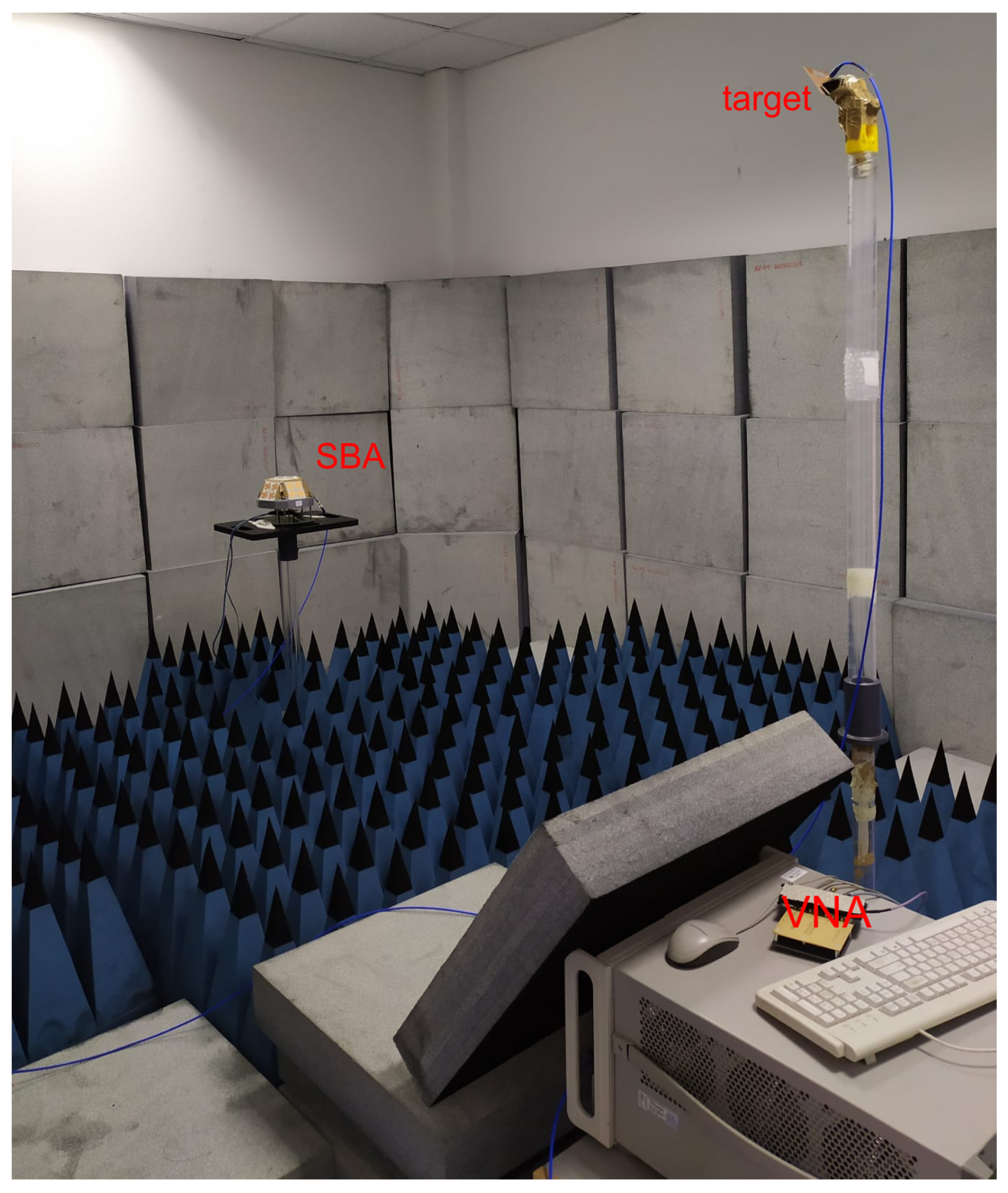
3.2. Experimental Setup

To prove the effectiveness of the method, a massive campaign of measurement was carried out in a semi-anechoic chamber scenario with the SBA anchor installed on a rotating platform controlled by a computer, thus spanning the entire azimuthal domain. Measurements were acquired through the utilization of a calibrated vector network analyzer (VNA), connected to a computer to get measurements synchronized with the SBA antenna switching, as depicted in Figure 10. The VNA equipment is able to provide a measurement of the radio-link transfer function as shown in Section 2.3. Synchronized measurement routines are used to fulfill the conditions on sampling periodicity as given in Section 2.3, Figure 4. Due to high communication times between computer and VNA, the synchronization condition is satisfied acquiring more than one signal period for each antenna measurement.

The adoption of the laboratory instrumentation is due to the need to remove all the possible cause of measurement uncertainty, and thus permits us to focus on the methodological aspects of this work. In particular, the validation of calibrated VNA as equivalent to time domain signal sampling was demonstrated by the authors of [15]. Figure 11 shows a picture of the laboratory set-up schematically represented in the Figure 10, which includes absorbing panels and the VNA hidden by the same panels; the SBA is installed in a rotating platform, while the target in positioned on a teflon pole and moved in different position and getting different heights. The target is emulated by only the transmitting antenna, which is identical to the SBA individual element; the reader can refer to the Table 1 for a summary of the transmitting antenna features.

Nevertheless, to prove method robustness towards a lack of synchronization between the signal transmission and signal reception in the experiment, a random time shift has been introduced in each set of time observations throughout the SBA antennas. Each time observation is given as the Inverse Fourier Transform of an $S_{21}$ measurement trace considering a bandwidth $\mathrm{B}=3\mathrm{GHz}$ centered in $f_0=5.5\mathrm{GHz}$ and a number of points $M=801$.

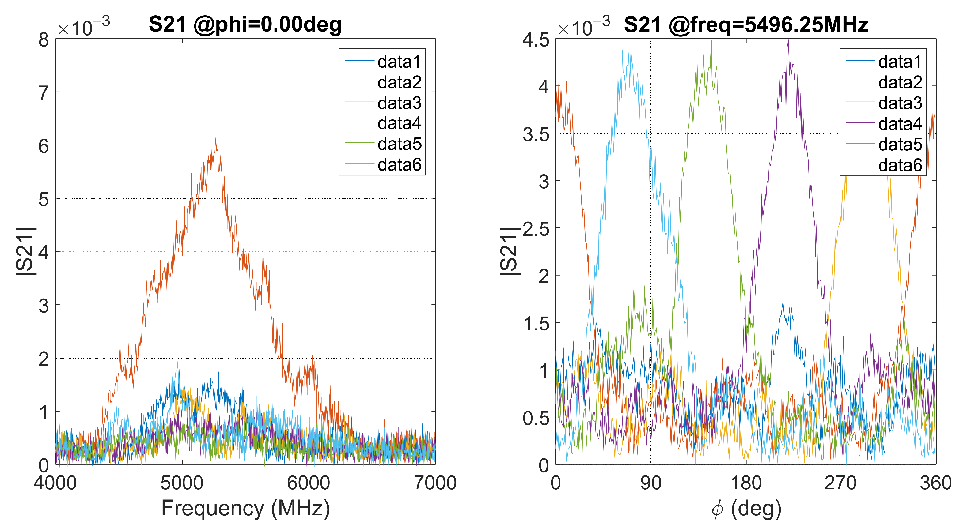
3.3. Experimental Measurements

In this section, we report the results of a massive campaign of measurements carried out putting the target emulated by the transmitting antenna on different heights and different distances; Figure 12 reports the entire set of target positions, with respect to the SBA anchor. An entire set of time observation was taken, for each target position and for a convenient number of SBA rotation angles, spanning the azimuthal domain $\phi$ with a step of $1\mathrm{deg}$.

In Figure 13 are shown the typical measured calibrated data composing a steering vector, acquired by the instrumentation in terms of the magnitude of the transmission parameter $S21$. By observing the plots we can easily observe from the data associated to the SBA element 2, that the effective antenna bandwidth is between 4.75 GHz to 6.25 GHz, thus justifying its use as reduced bandwidth defined herein above. Note that in this example, antenna 2 is the one aligned with the transmitting antenna, while the others result directed elsewhere according to the SBA geometry shown in Figure 6; still according with the SBA geometry antenna 1 points upward, that is $\theta =0$ degree and thus provides a low trace in the data plots. The second set of plots shown in Figure 13, provides instead the steering vector data at center frequency, as a function of the azimuthal angle. As expected, in this set of data the shapes of the curve resemble the one of the radiation diagram shown in Figure 6.

For each rotation the signal DoA and the related error estimations were estimated following the method introduced in Section 2.1, adopting the MUSIC ML estimator in its scalar implementation [21], dealing with phase-less steering vectors, and in its standard implementation [23,24], with phase-reconstructed data. To assess the validity of the phase reconstruction process, the estimations were also carried out using steering vectors completed with pure phase information related to the center frequency $f_0$. The results about all these cases are compared in the Figure 14 where are reported the CDFs for the obtained DoA estimation errors.

In particular, in Figure 14a,b the distribution functions are calculated with respect to each angle subject to estimation, while Figure 14c shows the combined estimation error considering the euclidean distance between the estimated DoA and the real one as

$${\epsilon }_{\mathrm{DoA}}=\sqrt{{(\widehat{\vartheta }-\vartheta )}^2+{(\widehat{\phi }-\phi )}^2}$$

(55)

with $\widehat{\vartheta },\widehat{\phi }$ being the estimated DoA values and $\vartheta ,\phi$ the actual ones.

By observing Figure 14 it is clear how much the proposed phase reconstruction method is able to recover a coherent phase information. This is especially noticeable when looking at the accuracy improvement on azimuthal domain $\phi$ (Figure 14b), where the introduction of center frequency phase information actually worsened overall results. This is coherent with results in Figure 8 where severe phase wrapping phenomena were expected along the azimuthal domain, especially for lower azimuth angles.

In the azimuthal direction the implementation of phase recovery did not lead to accuracy improvements but it prevented the disruption of steering vectors information. Conversely on elevation direction the re-introduction of phase allowed to overcome the lack of antenna elements due to SBA array geometry, giving an huge improvement on estimation accuracy, as shown in Figure 14a.

The experiment was repeated by considering the reduced bandwidth, 4.75–6.25 GHz, where the SBA antenna provides a maximally gain according to Table 1. The DoA estimation error in the reduced bandwidth is reported in the Figure 14c, in comparison with those carried out in the nominal bandwidth. From the data we can recognize that reducing the bandwidth, to that where the antenna performs better, the noise bandwidth reduces and the overall SNR increases thus leading to slightly better DoA accuracy. In the Figure 14c we can estimate that the CDF improves of 1.5% at 20 degree, while it remains constant at 10 degrees.

In addition to pure DoA estimations, the involvement of wide-band signals enables to calculate range estimations. Applying the method already proposed in [15], measuring the peak delay with respect to the transmission time range estimation is possible by simply calculating

$$R=c_0·{{\tau }_{\widetilde{\mathrm{PK}}}}_d=c_0\left({{\tau }_{\mathrm{PK}}}_d+t_0\right),$$

(56)

where d is the index of the antenna showing the maximum absolute peak value for its related time observation, ${{\tau }_{\mathrm{PK}}}_d$ is the time of arrival of peak, and $t_0$ is the signal transmission beginning time. Note that here the knowledge of $t_0$ parameter is mandatory, thus range estimations require an absolute synchronization between transmitter and receiver achievable through the VNA or applying specific signal coding schemes [42,43,44].

The range resolution is related to timing resolution, and the latter is approximable to inverse of signal bandwidth following signal condition shown in (40), so

$$\mathsf{\Delta }R=c_0·\mathsf{\Delta }{{\tau }_{\widetilde{\mathrm{PK}}}}_d\approx \frac{c_0}{\mathrm{B}}$$

(57)

where with a bandwidth $\mathrm{B}=3\mathrm{GHz}$ it results $\mathsf{\Delta }R\approx 10\mathrm{cm}$. Furthermore dealing with a one-way transmission there is not any issue related to range ambiguity.

Position estimation is calculated as

$$\overline{\mathbf{x}}=R·\left(\begin{array}{c}sin\widehat{\vartheta }cos\widehat{\phi }\\ sin\widehat{\vartheta }sin\widehat{\phi }\\ cos\widehat{\vartheta }\end{array}\right),$$

(58)

where $\left(\widehat{\vartheta },\widehat{\phi }\right)$ is the estimated DoA for each transmitting position respect the SBA reference system. The positioning error is calculated as the euclidean distance between estimation and real position. Figure 15 shows the CDF for both the range estimation error and the positioning error, being the latter a combination of the error due to range and angle estimations.

As shown by plots, a correct time offset compensation let the range estimation error to be comparable with range resolution, i.e., ≈10 cm. The CDFs of final position estimations follow the trends of Figure 14c, upholding the efficacy of the proposed phase reconstruction method.

Furthermore, in this case we report the positioning estimation carried out by considering the reduced operation bandwidth of 4.75–6.25 GHz. We see from the curves, that the range estimation exhibits a slight reduction of the accuracy, nominally at 0.1 m the CDF reduces of 3.7%, as result of the analysis bandwidth reduction. Nevertheless, the combined range—DoA positioning error maintains the same slight advantage from reduced noise bandwidth.

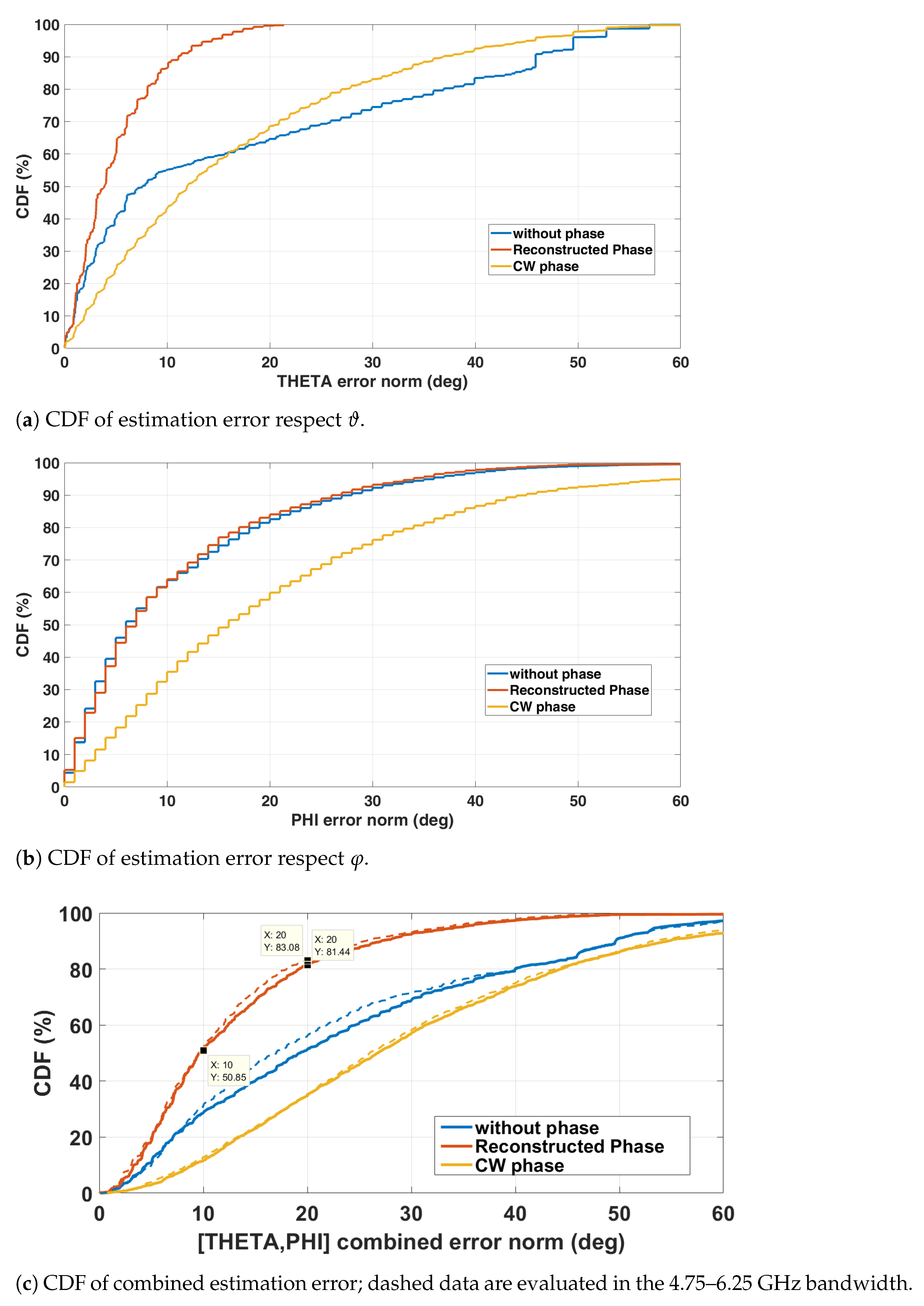
3.4. Simulated DoA Accuracy versus SNR

For the sake of a better comprehension of the experimental results, we report briefly the results of a set of simulations carried out by implementing the analytical model of Section 2.1 and applying the technique described in Section 2.3. During this analysis, we considered both the SBA and the transmitting antenna as implemented of radiators characterized by the features described in Table 1 and with the radiation pattern of Figure 6. We adopted the $awgn\{.\}$ function available in Matlab, which can estimate the incoming signal power and to add a proper level of white noise, such that the signal-to-noise ratio (SNR) reach a given value. The results of this analysis were conducted at different SNR levels, ranging from −15 dB to 10 dB, and the corresponding CDF curves are reported in Figure 16. From the CDF curve associated to SNR = −15 dB, we can recognize the shape already shown in Figure 14c; under a closer inspection, we see that the CDF values at errors 10 degree and 20 degree are in agreement for less than 3% with those experimentally derived. We can thus conclude that the overall SNR affecting the measurement is in the range of −15 dB, and that the analytical model is capable to reproduce with accuracy of less then 3% the DoA experiments. We should not be surprised about the capability of the method to recover the DoA estimate with good accuracy, because in spite the large bandwidth adopted, the method introduces a process gain due to inverse FFT involved in the phase reconstruction.

4. Conclusions

This work presented a new methodology for recovering phase information corrupted by phase wrapping issues on phase-impaired antenna arrays intended for DoA estimations. The proposed method resulted effective in fixing the loss of accuracy in DoA estimations, leading to an huge accuracy improvement as expected by the proper inclusion of the phase information.

The cost for this benefit is the involvement of wideband signals, but dealing with modern data communication protocols such drawback could be less cumbersome than expected. Furthermore, modern ultra-wideband (i.e., fraction bandwidth > 20%)-based systems often provide a time synchronization protocol which also enables range estimation capability thus allowing to implement complete and cost-effective positioning solutions.

An example of implementation based on calibrated VNA measurements has been shown, leaving to further investigation the development of a system capable of data communication, implementing the functionalities of systems shown in [16,22]. Nevertheless, this work has introduced also some design principles and algorithmic concepts useful for actual system development.

References

1. Guan, W.; Chen, S.; Wen, S.; Tan, Z.; Song, H.; Hou, W. High-accuracy robot indoor localization scheme based on robot operating system using visible light positioning. IEEE Photonics J. 2020, 12, 1–16. [Google Scholar] [CrossRef]
2. Guan, T.; Fang, L.; Dong, W.; Koutsonikolas, D.; Challen, G.; Qiao, C. Robust, cost-effective and scalable localization in large indoor areas. Comput. Netw. 2017, 120, 43–55. [Google Scholar] [CrossRef]
3. AlHajri, M.I.; Ali, N.T.; Shubair, R.M. Indoor localization for IoT using adaptive feature selection: A cascaded machine learning approach. IEEE Antennas Wirel. Propag. Lett. 2019, 18, 2306–2310. [Google Scholar] [CrossRef]
4. Khelifi, F.; Bradai, A.; Benslimane, A.; Rawat, P.; Atri, M. A survey of localization systems in internet of things. Mob. Netw. Appl. 2019, 24, 761–785. [Google Scholar] [CrossRef]
5. Sakpere, W.; Adeyeye Oshin, M.; Mlitwa, N. A State-of-the-Art Survey of Indoor Positioning and Navigation Systems and Technologies. S. Afr. Comput. J. 2017, 29, 145. [Google Scholar] [CrossRef] [Green Version]
6. Groth, M.; Nyka, K.; Kulas, L. Calibration-Free Single-Anchor Indoor Localization Using an ESPAR Antenna. Sensors 2021, 21, 3431. [Google Scholar] [CrossRef]
7. Kim, Y.J.; Kim, Y.B.; Dong, H.J.; Cho, Y.S.; Lee, H.L. Compact Switched-Beam Array Antenna with a Butler Matrix and a Folded Ground Structure. Electronics 2020, 9, 2. [Google Scholar] [CrossRef] [Green Version]
8. Giorgetti, G.; Cidronali, A.; Gupta, S.K.; Manes, G. Single-anchor indoor localization using a switched-beam antenna. IEEE Commun. Lett. 2009, 13, 58–60. [Google Scholar] [CrossRef] [Green Version]
9. Lee, C.U.; Noh, G.; Ahn, B.; Yu, J.W.; Lee, H.L. Tilted-beam switched array antenna for UAV mounted radar applications with 360deg coverage. Electronics 2019, 8, 1240. [Google Scholar] [CrossRef] [Green Version]
10. Zhang, H.; Zong, H.; Qiu, J. A Range Resolution Enhancement Algorithm for Active Millimeter Wave Based on Phase Unwrapping Mechanism. Electronics 2021, 10, 1689. [Google Scholar] [CrossRef]
11. Peng, H.; Zhi, R.; Yang, Q.; Cai, J.; Wan, Y.; Liu, G. Design of a MIMO Antenna with High Gain and Enhanced Isolation for WLAN Applications. Electronics 2021, 10, 1659. [Google Scholar] [CrossRef]
12. Rojhani, N.; Passafiume, M.; Lucarelli, M.; Collodi, G.; Cidronali, A. Exploiting Compressive Sensing Basis Selection to Improve 2 × 2 MIMO Radar Image. In Proceedings of the 2020 IEEE MTT-S International Conference on Microwaves for Intelligent Mobility (ICMIM), Linz, Austria, 23–23 November 2020; pp. 1–4. [Google Scholar]
13. Álvarez López, Y.; Rodríguez Vaqueiro, Y.; González Valdés, B.; Las Heras Andrés, F.L.; García Pino, A. Fourier-based imaging for subsampled multistatic arrays. IEEE Trans. Antennas Propag. 2016, 64, 2557–2562. [Google Scholar] [CrossRef] [Green Version]
14. Zhang, Y.; Gong, X.; Liu, K.; Zhang, S. Localization and Tracking of an Indoor Autonomous Vehicle Based on the Phase Difference of Passive UHF RFID Signals. Sensors 2021, 21, 3286. [Google Scholar] [CrossRef]
15. Cidronali, A.; Collodi, G.; Lucarelli, M.; Maddio, S.; Passafiume, M.; Pelosi, G. A Combined DoA-ToA Localization Technique Based on a Broadband Switched Beam Antenna. In Proceedings of the 2019 IEEE Conference on Antenna Measurements & Applications (CAMA), Kuta, Indonesia, 23–25 October 2019; pp. 210–213. [Google Scholar]
16. Passafiume, M.; Maddio, S.; Cidronali, A. An improved approach for RSSI-based only calibration-free real-time indoor localization on IEEE 802.11 and 802.15. 4 wireless networks. Sensors 2017, 17, 717. [Google Scholar] [CrossRef] [Green Version]
17. Zhao, L.; Wang, H.; Wang, J.; Gao, H.; Liu, J. Robust Wi-Fi indoor localization with KPCA feature extraction of dual band signals. In Proceedings of the 2017 IEEE International Conference on Robotics and Biomimetics (ROBIO), Macau, China, 5–8 December 2017; pp. 908–913. [Google Scholar]
18. Maddio, S.; Passafiume, M.; Cidronali, A.; Manes, G. A distributed positioning system based on a predictive fingerprinting method enabling sub-metric precision in IEEE 802.11 networks. IEEE Trans. Microw. Theory Tech. 2015, 63, 4567–4580. [Google Scholar] [CrossRef]
19. Wen, Y.; Tian, X.; Wang, X.; Lu, S. Fundamental limits of RSS fingerprinting based indoor localization. In Proceedings of the 2015 IEEE Conference on Computer Communications (INFOCOM), Hong Kong, China, 26 April–1 May 2015; pp. 2479–2487. [Google Scholar]
20. Werner, J.; Wang, J.; Hakkarainen, A.; Cabric, D.; Valkama, M. Performance and Cramer–Rao bounds for DoA/RSS estimation and transmitter localization using sectorized antennas. IEEE Trans. Veh. Technol. 2015, 65, 3255–3270. [Google Scholar] [CrossRef]
21. Passafiume, M.; Maddio, S.; Cidronali, A.; Manes, G. MUSIC algorithm for RSSI-based DoA estimation on standard IEEE 802.11/802.15. x systems. World Sci. Eng. Acad. Soc. Trans. Signal Process 2015, 11, 58–68. [Google Scholar]
22. Cidronali, A.; Collodi, G.; Maddio, S.; Passafiume, M.; Pelosi, G. 2-D DoA anchor suitable for indoor positioning systems based on space and frequency diversity for legacy WLAN. IEEE Microw. Wirel. Compon. Lett. 2018, 28, 627–629. [Google Scholar] [CrossRef]
23. Schmidt, R. Multiple emitter location and signal parameter estimation. IEEE Trans. Antennas Propag. 1986, 34, 276–280. [Google Scholar] [CrossRef] [Green Version]
24. Gupta, P.; Kar, S. MUSIC and improved MUSIC algorithm to estimate direction of arrival. In Proceedings of the 2015 International Conference on Communications and Signal Processing (ICCSP), Melmaruvathur, India, 2–4 April 2015; pp. 0757–0761. [Google Scholar]
25. Roy, R.; Kailath, T. ESPRIT-estimation of signal parameters via rotational invariance techniques. IEEE Trans. Acoust. Speech Signal Process. 1989, 37, 984–995. [Google Scholar] [CrossRef] [Green Version]
26. Cidronali, A.; Collodi, G.; Lucarelli, M.; Maddio, S.; Passafiume, M.; Pelosi, G. Assessment of Anchors Constellation Features in RSSI-Based Indoor Positioning Systems for Smart Environments. Electronics 2020, 9, 1026. [Google Scholar] [CrossRef]
27. Cidronali, A.; Ciervo, E.; Collodi, G.; Maddio, S.; Passafiume, M.; Pelosi, G. Analysis of Dual-Band Direction of Arrival Estimation in Multipath Scenarios. Electronics 2021, 10, 1236. [Google Scholar] [CrossRef]
28. Maddio, S.; Cidronali, A.; Passafiume, M.; Collodi, G.; Lucarelli, M.; Maurri, S. Multipath robust azimuthal direction of arrival estimation in dual-band 2.45–5.2 GHz networks. IEEE Trans. Microw. Theory Tech. 2017, 65, 4438–4449. [Google Scholar] [CrossRef]
29. Cidronali, A.; Collodi, G.; Lucarelli, M.; Maddio, S.; Passafiume, M.; Pelosi, G. An IEEE 802. 15. 4 Wireless Half-Cubic Node Based on a Switched-Beam Antenna for Indoor Direction of Arrival Estimation. In Proceedings of the 2020 17th European Radar Conference (EuRAD), Utrecht, The Netherlands, 10–15 January 2021; pp. 286–289. [Google Scholar]
30. Cidronali, A.; Collodi, G.; Lucarelli, M.; Maddio, S.; Passafiume, M.; Pelosi, G. Continuous Beam Steering For Phaseless Direction-of-Arrival Estimations. IEEE Antennas Wirel. Propag. Lett. 2019, 18, 2666–2670. [Google Scholar] [CrossRef]
31. Hou, Y.; Yang, X.; Abbasi, Q.H. Efficient AoA-based wireless indoor localization for hospital outpatients using mobile devices. Sensors 2018, 18, 3698. [Google Scholar] [CrossRef] [PubMed] [Green Version]
32. Maddio, S.; Cidronali, A.; Passafiume, M.; Collodi, G.; Maurri, S. Fine-grained azimuthal direction of arrival estimation using received signal strengths. Electron. Lett. 2017, 53, 687–689. [Google Scholar] [CrossRef]
33. Rojhani, N.; Passafiume, M.; Lucarelli, M.; Collodi, G.; Cidronali, A. Assessment of Compressive Sensing 2 × 2 MIMO Antenna Design for Millimeter-Wave Radar Image Enhancement. Electronics 2020, 9, 624. [Google Scholar] [CrossRef] [Green Version]
34. Cidronali, A.; Passafiume, M.; Colantonio, P.; Collodi, G.; Florian, C.; Leuzzi, G.; Pirola, M.; Ramella, C.; Santarelli, A.; Traverso, P. System level analysis of millimetre-wave gan-based mimo radar for detection of micro unmanned aerial vehicles. In Proceedings of the 2019 PhotonIcs & Electromagnetics Research Symposium-Spring (PIERS-Spring), Rome, Italy, 17–20 June 2019; pp. 438–450. [Google Scholar]
35. Levis, C.; Johnson, J.T.; Teixeira, F.L. Radiowave Propagation: Physics and Applications; John Wiley & Sons: Hoboken, NJ, USA, 2010. [Google Scholar]
36. Cidronali, A.; Maddio, S.; Passafiume, M.; Manes, G. Car talk: Technologies for vehicle-to-roadside communications. IEEE Microw. Mag. 2016, 17, 40–60. [Google Scholar] [CrossRef]
37. Bras, L.; Carvalho, N.; Pinho, P.; Kulas, L.; Nyka, K. A Review of Antennas for Indoor Positioning Systems. Int. J. Antennas Propag. 2012, 2012, 1–14. [Google Scholar] [CrossRef]
38. Maddio, S.; Cidronali, A.; Manes, G. Smart Antennas for Direction-of-Arrival Indoor Positioning Applications. In Handbook of Position Location: Theory, Practice, and Advances; Wiley-IEEE Press: Piscataway, NJ, USA, 2011; pp. 319–355. [Google Scholar]
39. Maddio, S.; Pelosi, G.; Selleri, S. Circularly polarised sequential array with enhanced gain and bandwidth for applications in C-band. IET Microw. Antennas Propag. 2020, 14, 1926–1932. [Google Scholar] [CrossRef]
40. Maddio, S. A compact circularly polarized antenna for 5.8-GHz intelligent transportation system. IEEE Antennas Wirel. Propag. Lett. 2016, 16, 533–536. [Google Scholar] [CrossRef]
41. Maddio, S.; Passafiume, M.; Cidronali, A.; Manes, G. Impact of the dihedral angle of switched beam antennas in indoor positioning based on RSSI. In Proceedings of the 2014 11th European Radar Conference, Rome, Italy, 8–10 October 2014; pp. 317–320. [Google Scholar] [CrossRef]
42. Barral, V.; Escudero, C.J.; García-Naya, J.A.; Maneiro-Catoira, R. NLOS identification and mitigation using low-cost UWB devices. Sensors 2019, 19, 3464. [Google Scholar] [CrossRef] [PubMed] [Green Version]
43. Ridolfi, M.; Vandermeeren, S.; Defraye, J.; Steendam, H.; Gerlo, J.; De Clercq, D.; Hoebeke, J.; De Poorter, E. Experimental evaluation of UWB indoor positioning for sport postures. Sensors 2018, 18, 168. [Google Scholar] [CrossRef] [Green Version]
44. Deng, H.; Himed, B.; Wicks, M.C. Concurrent extraction of target range and Doppler information by using orthogonal coding waveforms. IEEE Trans. Signal Process. 2007, 55, 3294–3301. [Google Scholar] [CrossRef]
Figure 1. Scheme of an ideal Uniform Circular Array in a tridimensional space.
Electronics 10 02137 g001
Figure 2. Example of a generic multi-tone signal with constant tones amplitude and Sine Fit.
Electronics 10 02137 g002
Figure 3. Example of a set of impinging multi-tone signals on an array.
Electronics 10 02137 g003
Figure 4. Scheme of an IQ demodulator switched beam array-based receiver chain.
Electronics 10 02137 g004
Figure 5. The assembled SBA of the anchor device adopted in the experiments (left), detail of the single array element (right).
Electronics 10 02137 g005
Figure 6. Radiation pattern of each SBA element.
Electronics 10 02137 g006
Figure 7. Pictorial representation of the observation model for the experiment.
Electronics 10 02137 g007
Figure 8. Ideal and wrapped phase differences respect to reference antenna #1.
Electronics 10 02137 g008
Figure 9. Ideal phase differences respect to reference antenna #1 for frequency fit f FIT = B M .
Electronics 10 02137 g009
Figure 10. Block diagram of the experiment setup. The transmitting antenna emulates the target.
Electronics 10 02137 g010
Figure 11. Picture of the experimental setup with the target positioned on a pole and the SBA installed on a rotating platform.
Electronics 10 02137 g011
Figure 12. Schematic diagram of the SBA and transmitting antennas experimental relative positions.
Electronics 10 02137 g012
Figure 13. Example of measured S21 parameter for entire set of 6 SBA elements, labeled ‘data { n } ’, with transmitting antenna positioned at height: 280 cm, range 220 cm. Data acquired across the nominal frequency bandwidth (left) at ϕ = 0 deg, and across the entire azimuthal domain at center frequency band (right).
Electronics 10 02137 g013
Figure 14. Cumulative Distribution Functions (CDFs) of experimental DoA estimations error.
Electronics 10 02137 g014
Figure 15. Cumulative distribution function for range estimation error and positioning error; dashed curves are related to estimation in the 4.75–6.25 GHz frequency band.
Electronics 10 02137 g015
Figure 16. Simulated cumulative distribution function for combined 2-D DoA as a function of signal to noise ratio.
Electronics 10 02137 g016