Adaptive Transfer Learning Based on a Two-Stream Densely Connected Residual Shrinkage Network for Transformer Fault Diagnosis over Vibration Signals

Abstract

Vibration signal analysis is an efficient online transformer fault diagnosis method for improving the stability and safety of power systems. Operation in harsh interference environments and the lack of fault samples are the most challenging aspects of transformer fault diagnosis. High-precision performance is difficult to achieve when using conventional fault diagnosis methods. Thus, this study proposes a transformer fault diagnosis method based on the adaptive transfer learning of a two-stream densely connected residual shrinkage network over vibration signals. First, novel time-frequency analysis methods (i.e., Synchrosqueezed Wavelet Transform and Synchrosqueezed Generalized S-transform) are proposed to convert vibration signals into different images, effectively expanding the samples and extracting effective features of signals. Second, a Two-stream Densely Connected Residual Shrinkage (TSDen2NetRS) network is presented to achieve a high accuracy fault diagnosis under different working conditions. Furthermore, the Residual Shrinkage layer (RS layer) is applied as a nonlinear transformation layer to the deep learning framework to remove unimportant features and enhance anti-interference performance. Lastly, an adaptive transfer learning algorithm that can automatically select the source data set by using the domain measurement method is proposed. This algorithm accelerates the training of the deep learning network and improves accuracy when the number of samples is small. Vibration experiments of transformers are conducted under different operating conditions, and their results show the effectiveness and robustness of the proposed method.

1. Introduction

With the rapid development of digital power grids, research on intelligent, efficient, and comprehensive fault diagnosis methods guarantees the building of future power grids. Transformers are the most important electrical equipment in power grid systems; hence, their failure causes considerable economic losses [1]. However, the probability of such failure increases remarkably given the influences of natural disasters, the aging and mechanical deformation of transformers, and other factors [2,3]. Relying only on preventive tests and regular maintenance cannot meet the safety requirements of grid systems. To avoid the occurrence of malignant accidents, research on transformer fault state assessment technology, which exhibits scientific value and economic significance, must be conducted.

As is known to all, the fault diagnosis methods of transformers primarily include Dissolved Gas Analysis (DGA) [4], Short-circuit Reactance (SCR) [5], Infrared Thermography (IRT) [6,7], Frequency Response Analysis (FRA) [8,9], and so on. These traditional diagnostic methods are hysteretic and cannot diagnose faults before they occur.

However, the transformer vibration-based method is a relatively potential field [10]. The vibration amplitude and frequency spectrum can reflect the operation state of the transformer and realize early fault diagnosis. In addition, the vibration-based fault diagnosis method has many technical advantages. First, it does not need to change the operating state of the transformer and is easy to install. Second, it can track changes in the transformer’s operating state in real-time with high monitoring sensitivity.

Existing diagnostic methods can be divided into model-based methods and data-driven methods. The model-based methods are to describe the health status of transformers using physical or mathematical methods [11]. Hong et al. proposed four vibration-based methods to evaluate the health status of the transformer [12]. However, the physical and mathematical parameters of the transformer vary with operating conditions, so it is difficult to establish a diagnostic model only by physical or mathematical methods. The data-driven methods are to realize fault diagnosis by using machine learning techniques, which mainly include feature extraction methods and diagnosis models. The feature extraction methods are to extract useful and non-redundant features of the original data, which can reveal the specific differences between different faults. At present, the feature extraction methods mainly include the Short-time Fourier Transform (STFT), Hilbert–Huang Transform [13,14], Variational Mode Decomposition (VMD) [15], Wavelet Transform (WT) [16], Synchrosqueezed Wavelet Transform (SWT) [17,18,19]. However, due to the nonlinearity and high noise of the transformer vibration signals, it is difficult to achieve high-precision fault diagnosis only by traditional feature extraction methods.

The current diagnosis methods mainly include shallow intelligent diagnosis methods and deep learning diagnosis methods. The shallow intelligent diagnosis methods include Support Vector Machine (SVM), K-Nearest Neighbor (KNN) [20], and Relevance Vector Machine (RVM), etc. In [20], Zhang et al. proposed the SVM-KNN method for visual category recognition. In [21], Zhao et al. proposed a fault diagnosis method, which used the Multiple Kernel Support Vector Machine (MKSVM) method to realize fault diagnosis. In the work of [22], Wang et al. proposed the multiple kernel RVM method to classify transformer faults.

Deep learning diagnosis methods mainly include: DBN [23], SAE [24], CNN [25,26,27], ResNet [28,29], DenseNet [30,31,32], Res2Net [33,34], etc. In [23], Hinton et al. proposed the DBN method, which can establish a joint distribution between observation data and labels. In [24], Wen et al. used a three-layer sparse autoencoder to extract the features of the original data. In addition, anti-interference networks have recently been used for fault diagnosis. In [29], Zhao et al. proposed a soft thresholding layer inserted into the ResNet architecture for fault diagnosis, but it cannot accurately extract enough multiscale features and reduce network computation. As a branch of deep learning methods, transfer learning is developing rapidly and can be used to improve the accuracy of deep learning with small sample data. Moreover, in recent fault diagnosis research, the original data has been visualized and combined with the CNN method for fault diagnosis. In the work of [35], He et al. proposed generative adversarial networks with comprehensive wavelet features for fault diagnosis. In [36], Chen et al. proposed a novel domain adversarial transfer network to deal with large distribution difference domains. In [37], Liu et al. proposed a general transfer learning network under small samples, but it cannot adaptively select source data sets to improve the intelligent performance of the network.

Based on the above analysis, the current fault diagnosis methods generally have the following limitations.

(1)

In terms of feature extraction, transformer signals are extremely complicated due to their different vibration sources. Moreover, a transformer typically works in a strong interference environment, leading to many redundant signals. However, existing diagnosis methods usually compress signals to high dimensions or use traditional methods to extract features. Consequently, important fault features are easily lost, and the extracted features are not sufficiently comprehensive;

(2)

Fault diagnosis methods mostly include shallow and deep learning diagnosis methods at present. Traditional shallow fault diagnosis methods cannot completely distinguish fault features from signal signatures due to their simple network characteristics. Meanwhile, traditional deep learning diagnosis methods improve the capability to process complex signals, but they are prone to overfitting when dealing with small and unbalanced sample data.

Therefore, to address the problems above, this paper proposes an adaptive transfer learning method based on a two-stream densely connected residual shrinkage network for transformer fault diagnosis. The major contributions are as follows:

(1)

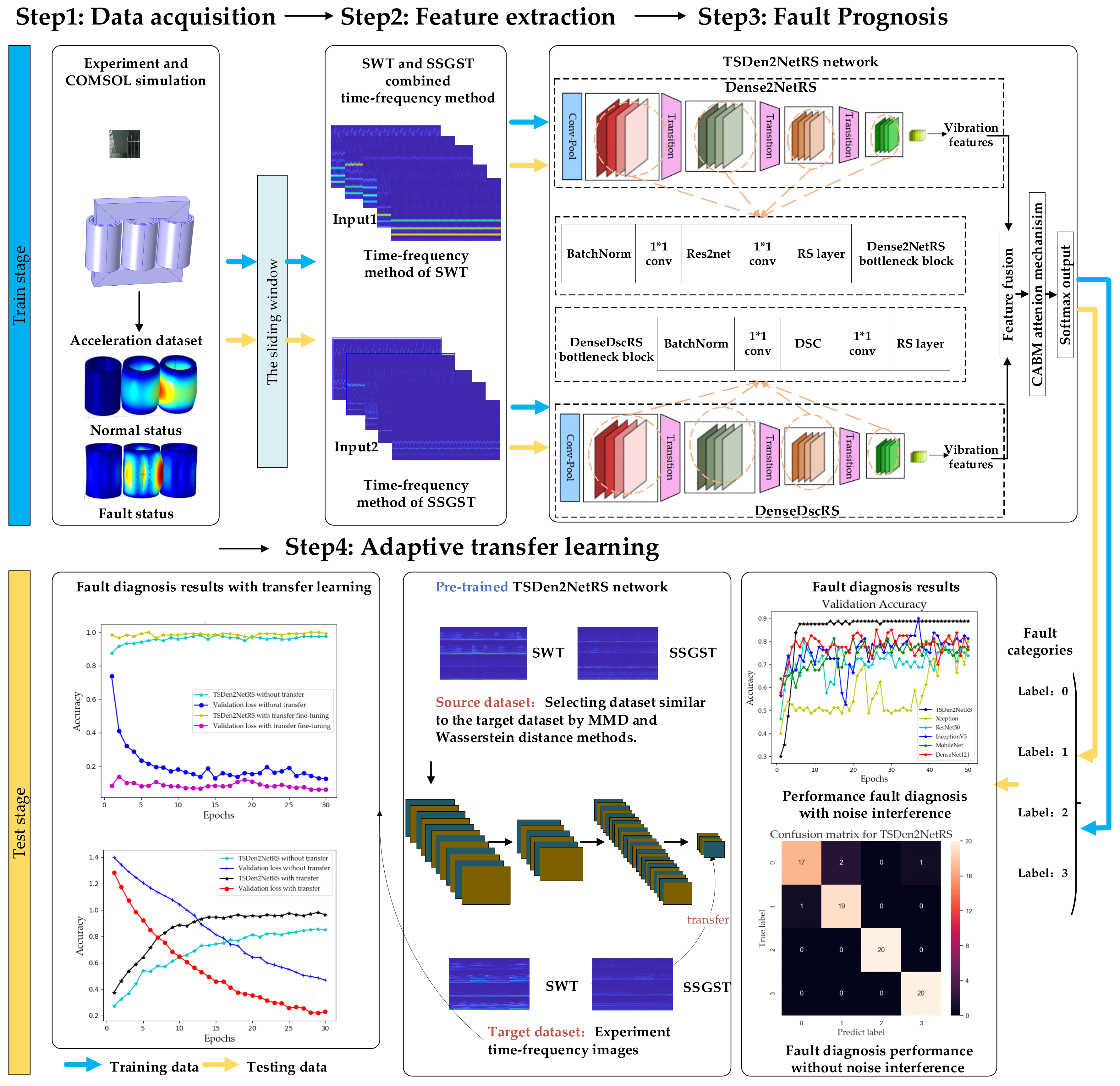
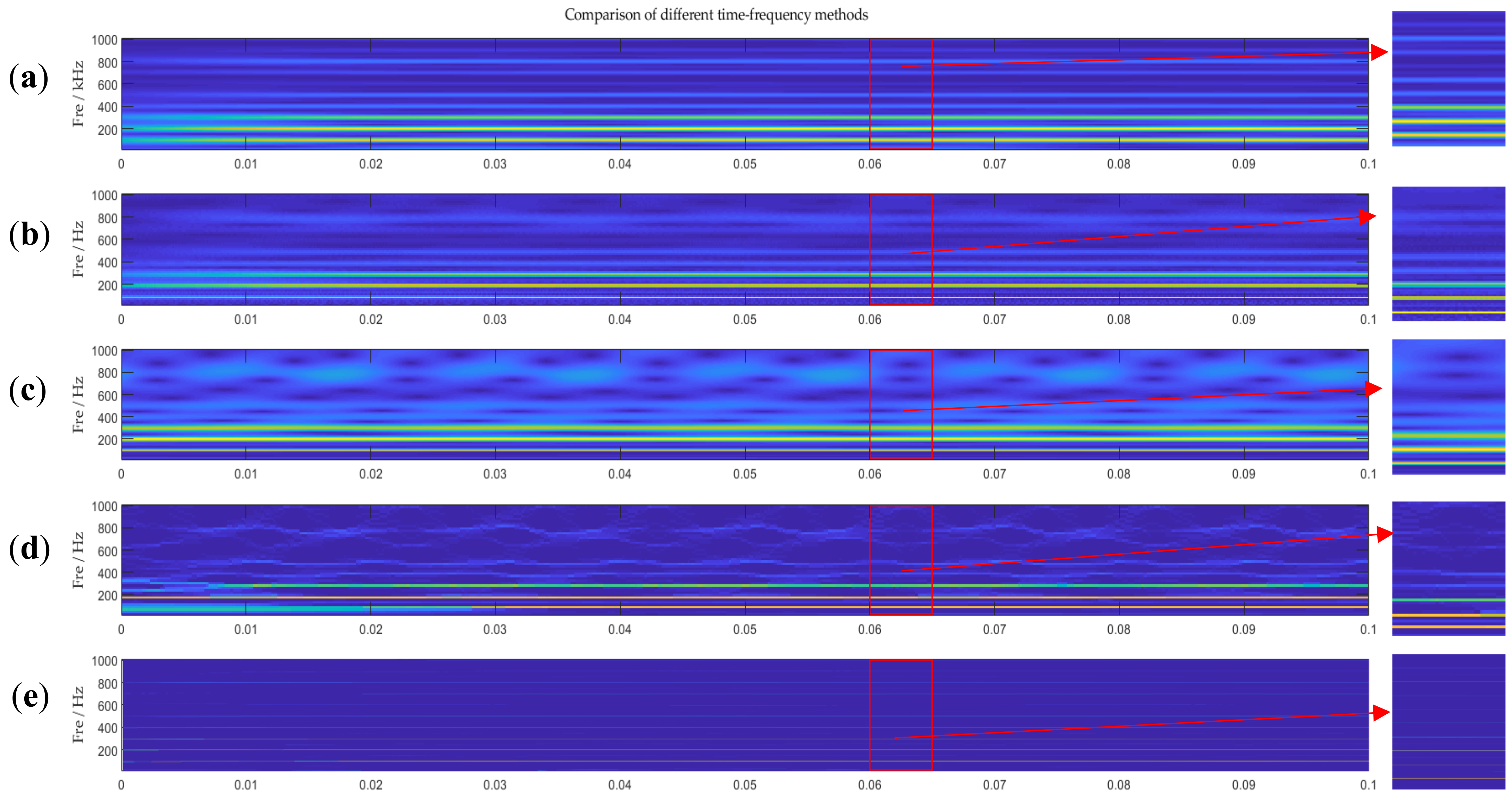
The SWT and Synchrosqueezed Generalized S-transform (SSGST) combined time-frequency method inherits the advantages of SWT and SSGST. Thus, energy concentration is improved compared with that of the traditional time-frequency methods, and the limitation of fuzzy time-frequency representation is overcome. Given these advantages, the feature extraction capability can be effectively improved. Moreover, the combined time-frequency analysis method converts the vibration signals into different time-frequency images, increasing the number of time-frequency features and alleviating the overfitting of deep learning.

(2)

A novel Two-stream Densely Connected Residual Shrinkage (TSDen2NetRS) network is proposed to realize fault diagnosis. The network not only has multiscale signal analysis capability but also uses a lightweight hybrid network to reduce computation and memory costs. Furthermore, the proposed method with a residual shrinkage layer can automatically filter out unimportant interference signals, realize feature recalibration, and improve anti-interference performance.

(3)

An adaptive transfer learning method is applied to transformer fault diagnosis; it can automatically select the source data set by using the domain measurement method and improve recognition capability under small samples.

The remainder of this paper is structured as follows. Section 2 illustrates the proposed method. Section 3 introduces the data acquisition and processing method. Section 4 presents the results and comparisons. Section 5 provides the conclusions.

2. Proposed Method

The architecture of the proposed fault diagnosis method is shown in Figure 1, which mainly includes the following steps:

Step1: Data acquisition. The transformer vibration signals of different fault types, locations, and severities are obtained through experiments and COMSOL finite element simulation software [38,39,40,41,42,43].

Step2: Feature extraction. The signals acquired are divided into several segments by the sliding window method, and then the segmented data is transformed into time-frequency images via the Synchrosqueezed Wavelet Transform (SWT) and Synchrosqueezed Wavelet Transform (SSGST) combined method.

Step3: Fault diagnosis. The multiple SWT and SSGST time-frequency images are divided into testing data set, validation data set, and training data set, which are the inputs of the Two-stream Densely Connected Residual Shrinkage (TSDen2NetRS) network. Meanwhile, the output features of the network are fused by the fusion method based on the Convolutional Block Attention Module (CABM). Finally, the transformer fault diagnosis based on vibration signal is realized.

Step4: Adaptive Transfer learning. The adaptive transfer learning method is used to automatically select the source data set by using the domain measurement method and pre-train the TSDen2NetRS network by the selected source data set. The following sections introduce the four steps in detail.

2.1. SWT and SSGST Combined Time-Frequency Analysis Method

The sliding window overlapping sampling method and the novel time-frequency analysis method are combined to transform the vibration signals into time-frequency images, and the images are used as the input of the deep learning network to realize the transformer fault diagnosis. The process is shown in Figure 2.

Step1: The sliding window overlapping sampling method transforms the time series into different observation segments to expand the data set. Each segment is a short time series of 0.02 s, and 40 observation points in each segment are selected for time-frequency transformation (in this article $point=1,2\cdots 40)$.

Step2: The SWT and SSGST combined method transforms the signals into time-frequency images.

(1)

The theory of the SWT method is explained in detail. The Continuous Wavelet Transform (CWT) of the signal $X\left(t\right)$ is defined as

$$W_X\left(u,h\right)=\frac{1}{\sqrt{u}}\underset{-\infty }{\overset{+\infty }{{\displaystyle \int }}}X\left(t\right){\psi }^{\ast }\left(\frac{t-h}{u}\right)dt$$

(1)

where $u$ is the scale expansion factor; $h$ is the translation factor; $\frac{1}{\sqrt{u}}\psi \left(\frac{t-h}{u}\right)$ is the wavelet basis function. Instantaneous frequency is estimated by deriving the wavelet coefficients. The formula is expressed as

$$\omega \left(u,h\right)=\left\{\begin{array}{c}-i{W}_X{\left(u,h\right)}^{-1}\frac{\partial W_X\left(u,h\right)}{{\partial }_h} W_X\left(u,h\right)\ne 0\\ \infty W_X\left(u,h\right)=0\end{array}\right.$$

(2)

where $i$ is the imaginary unit. SWT refers to use a compression algorithm to transfer the time-scale plane to the time-frequency plane and rearrange the energy. The SWT formula is

$$W{T}_X\left({\omega }_l,h\right)={\left(\Delta \omega \right)}^{-1}{{\displaystyle \sum }}_{u_{k:}\left|\omega \left(u_k,h\right)-{\omega }_l\right|\le \frac{\Delta \omega }{2}}{W}_X\left(u_k,h\right)u_k^{-\frac{3}{2}}{\left(\Delta u\right)}_k$$

(3)

where$u_k$ is the discrete scale; $k$ is the number of scales; ${\omega }_l=l·\frac{f_n}{N},l\in \left[1,N\right]$, ${\omega }_l$ is the center frequency, $f_n$ is the sampling frequency, $N$ is the total number of scales; $\Delta \mathsf{\omega }={\omega }_l-{\omega }_{l-1}=\frac{f_n}{N}$ and ${\left(\Delta u\right)}_k=u_k-u_{k-1}$. Compared with the CWT method, the SWT method has more concentrated energy in the spectrum and higher frequency resolution.

(2)

The SSGST method is presented in detail. The Generalized S-transform (GST) of the signal $X\left(t\right)$ is defined as

$$S_X\left(f,h\right)={{\displaystyle \int }}_{-\infty }^{+\infty }X\left(t\right)\frac{\lambda {\left|f\right|}^m}{{\left(2\pi \right)}^{\frac{1}{2}}}exp\left(-\frac{{\lambda }^2{f}^{2m}{\left(t-h\right)}^2}{2}\right)exp\left(-i2\pi ft\right)dt$$

(4)

where $f$ is the frequency;$m$ and $\lambda$ are the parameters for transforming the standard S-transform window function. The value of the frequency near the center frequency [$f_s-\frac{1}{2}{f}_o,f_s+\frac{1}{2}{f}_o$] is squeezed to the center frequency $f_s$, and $f_o$ is the frequency interval. The SSGST method is expressed as

$$S{T}_X\left(f_s,h\right)=f_o^{-1}{{\displaystyle \sum }}_{f_k:\left|f_s\left(f_k,h\right)-f_s\right|\le \frac{f_o}{2}}\left|S_X\left(f_k,h\right)\right|f_k\Delta f_k$$

(5)

where $f_k$ is the discrete frequency of generalized S-transform$, \Delta f_k=f_k-f_{k-1}.$

(3)

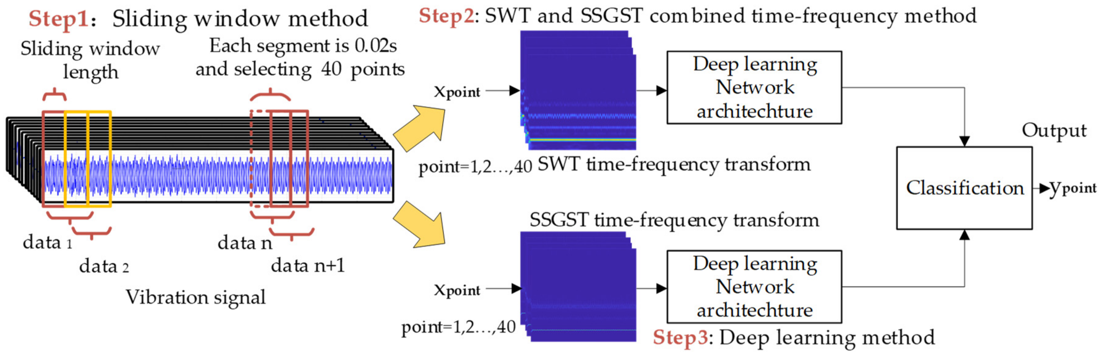
The theory of the SWT and SSGST combined method is illustrated in detail. The data processed by the sliding window method is transformed into time-frequency images by the SWT and SSGST combined methods. It can be calculated as

$$\left\{\begin{array}{c}{Y}_j\stackrel{SWT}{\to }{T}_Y{}_j\\ Y_j\stackrel{SSGST}{\to }{T}_{Y_j}^{\text{'}}\end{array}\right.\left(j=1,2\dots N_d\right)$$

(6)

where $Y_j$ is the data segmented by the sliding window method; $N_d$ is the amount of data after segmentation;$T_Y{}_j$ is the data transformed by SWT, and $T_{Y_j}^{\text{'}}$ is the data transformed by SSGST.

2.2. The Proposed Novel Deep Learning Method

The deep learning method proposed in this paper needs to solve these problems. First, due to the change of transformer’s load, environmental interference, and sampling frequency, the vibration signal scale will also change, so the ability to analyze multiscale signals needs to be considered. Second, the traditional deep learning methods are very redundant, resulting in very large computational and memory costs. The proposed method needs to consider efficient, lightweight deep learning methods, which mainly include group convolution and depthwise separable convolution. Finally, transformers usually operate in harsh interference environments, so the deep learning method proposed in this paper needs strong anti-interference performance.

2.2.1. TSDen2Net

The two-stream efficient densely connected convolutional network is proposed in this paper, named TSDen2Net, and this network architecture is from scratch. Compared with the existing traditional methods, the proposed method mainly has the following contributions:

(1)

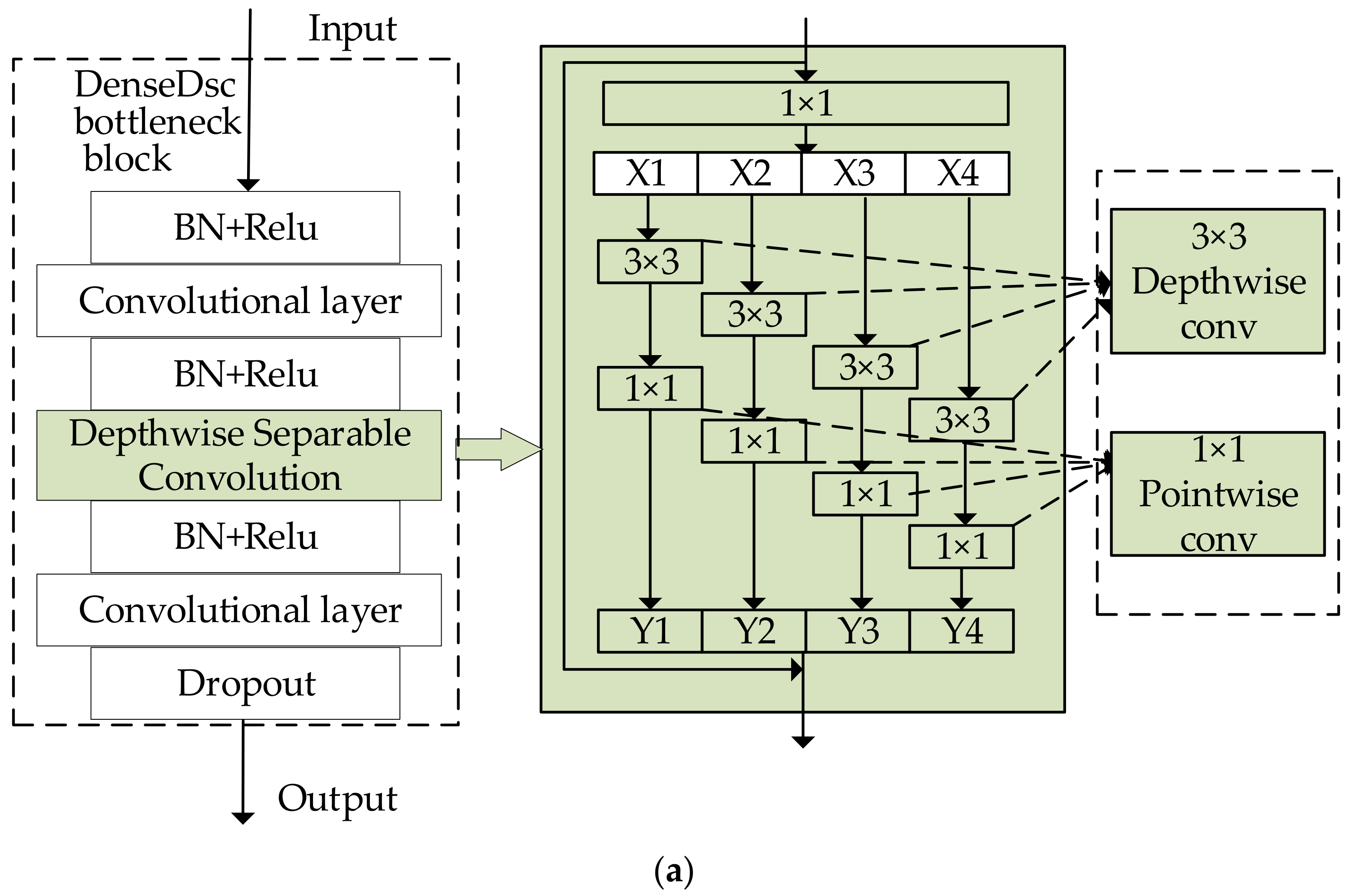
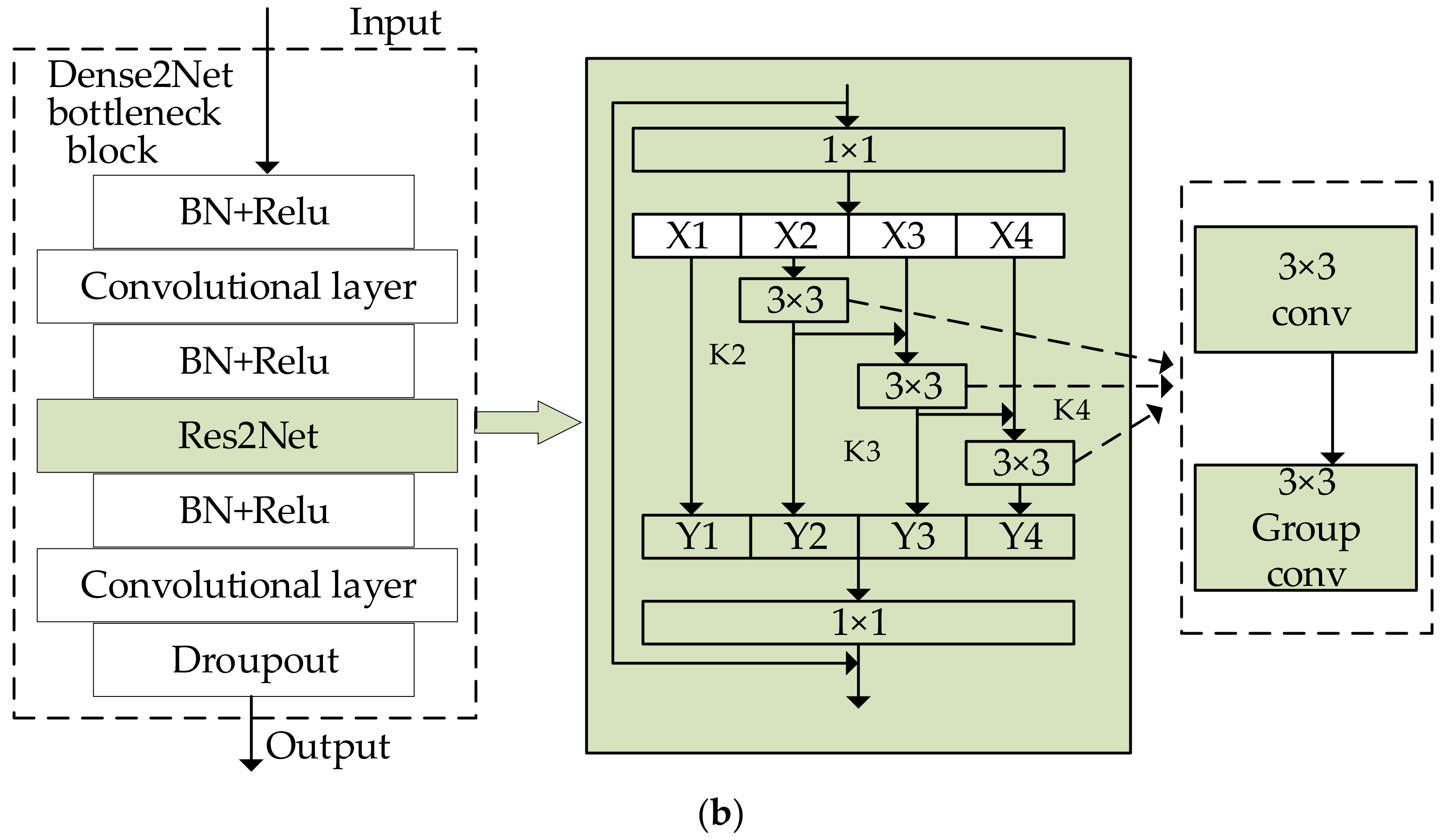
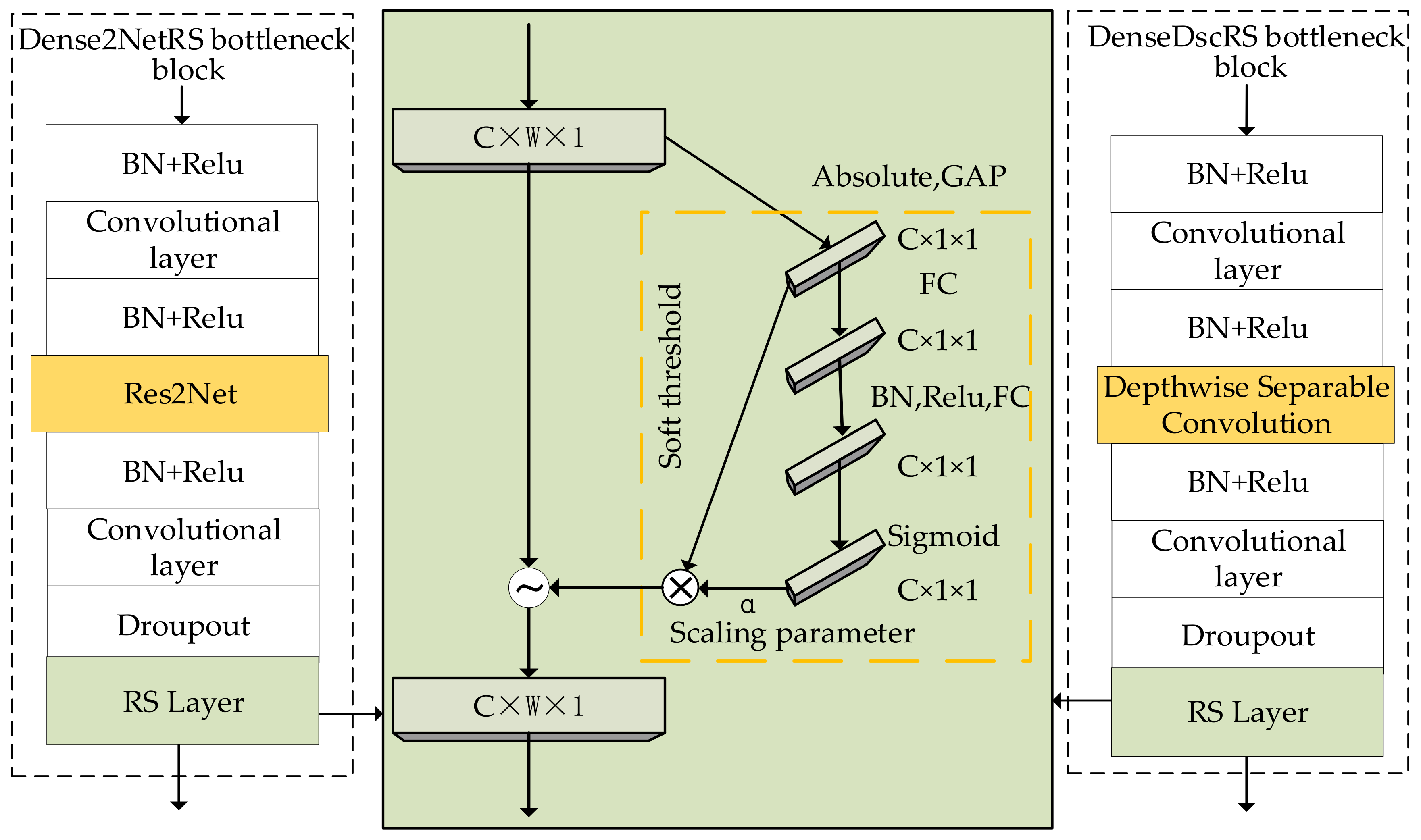
First, we construct two efficient densely connected convolutional networks. Depthwise separable convolution is applied to optimize the DenseNet network [30], named DenseDsc. The original bottleneck block of DenseNet is replaced by four parallel depthwise separable convolutions, and the novel block is called the DenseDsc bottleneck block, which is presented in Figure 3a. Meanwhile, Res2Net, proposed by Gao et al., is used to improve the DenseNet network [34], called Dense2Net. The standard bottleneck block of Dense2Net is replaced by Res2Net, and the block is named Dense2Net bottleneck block, as is illustrated in Figure 3b.

(2)

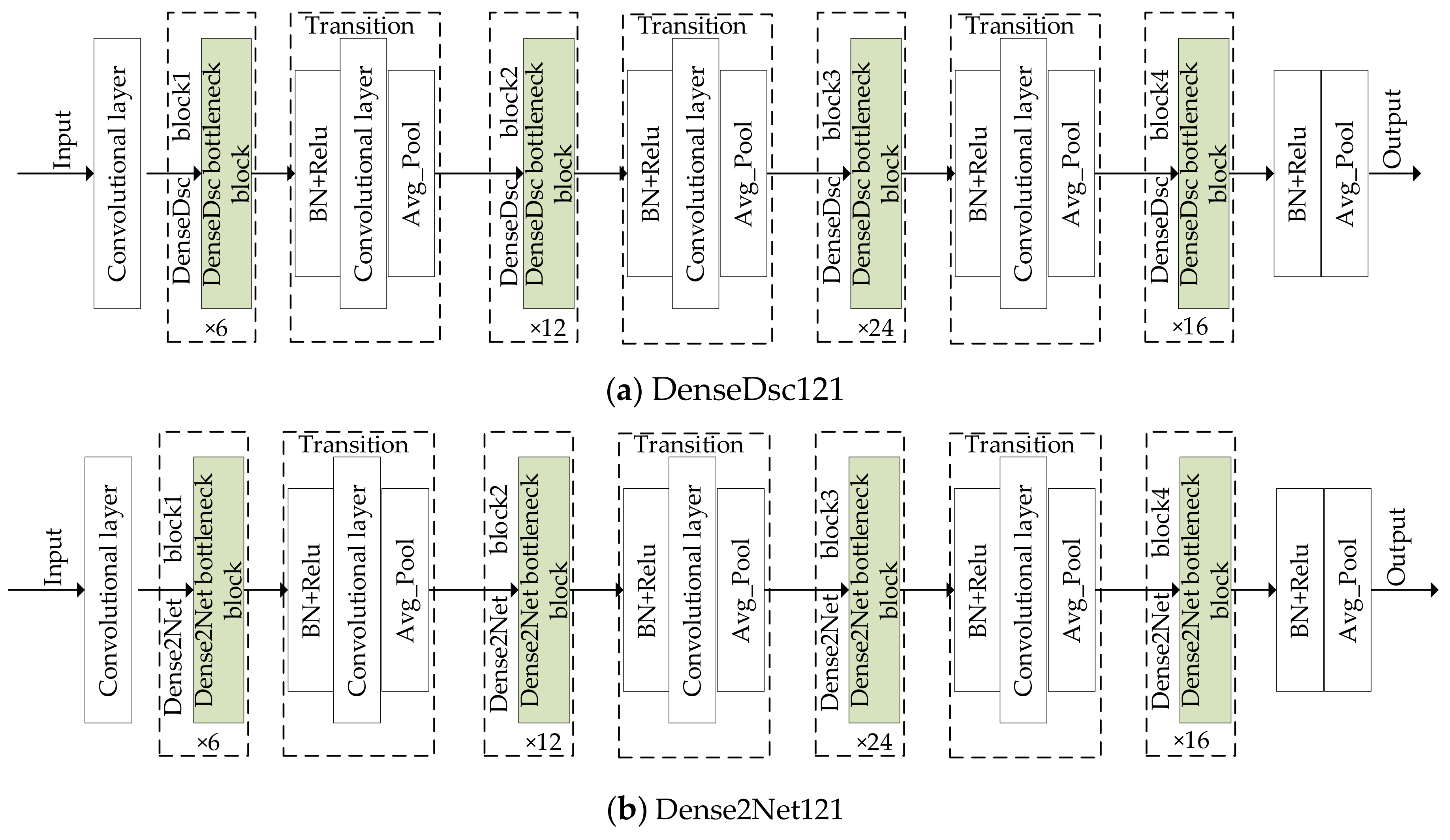
Then, due to the complex vibration time-frequency images of the transformer, we use deeper DenseDsc and Dense2Net, which are structured similar to the DenseNet121 network, named DenseDsc121 and Dense2Net121. The overall architecture is shown in Figure 4. The DenseDsc121 and Dense2Net121 both have 4 DenseDsc blocks and 3 transition layers. Further, the DenseDsc block shown in Figure 4, which is densely connected by multiple DenseDsc bottleneck blocks. The Dense2Net block shown in Figure 4 is densely connected by multiple Dense2Net bottleneck blocks.

(3)

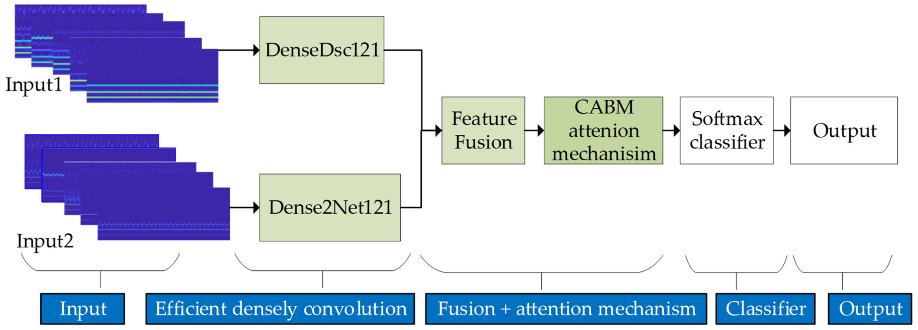
In order to extract features from different scales, we use DenseDsc121 and Dense2Net121 to construct a two-stream network named TSDen2Net. Its overall architecture is shown in Figure 5, and the network structure is shown in

Table 1. TSDen2Net network.

Layer Name	Output	DenseDsc	Dense2Net
Conv1	64 × 64	3 × 3, stride 1	3 × 3, stride 1
Dense Block1	64 × 64	DenseDsc × 6	Dense2Net × 6
Transition layer	32 × 32	Conv 1 × 1 and Average pool, stride 2	Conv 1 × 1 and Average pool, stride 2
Dense Block2	32 × 32	DenseDsc × 12	Dense2Net × 12
Transition layer	16 × 16	Conv 1 × 1 and Average pool, stride 2	Conv 1 × 1 and Average pool, stride 2
Dense Block3	16 × 16	DenseDsc × 24	Dense2Net × 24
Transition layer	8 × 8	Conv 1 × 1 and Average pool, stride 2	Conv 1 × 1 and Average pool, stride 2
Dense Block4	8 × 8	DenseDsc × 16	Dense2Net × 16
Pooling	4 × 4	Average pool, stride 2	Average pool, stride 2
Concatenate	-	Concatenate
CABM	-	Channel and attention spatial attention
Classification	-	FC and softmax

. The two-stream method can extract information at different scales and supplement the lack of effective information, which is conducive to improving the accuracy considerably.

2.2.2. TSDen2NetRS

In this paper, we used a new novel soft thresholding layer to reduce the interference, which is called the Residual Shrinkage layer (RS layer) [29]. The TSDen2Net network with the RS layer is named TSDen2NetRS. The RS layer overall architecture is shown in Figure 6, where C is the number of channels and W is the width of the feature map.

The RS layer is added at the end of the Dense2Net bottleneck block and the DenseDsc bottleneck block, which are named Dense2NetRS bottleneck block and DenseDscRS bottleneck block in this paper. It can automatically obtain the threshold of each channel according to the characteristics of the signals. The process is shown in Figure 6. The feature map is reduced to a 1-D vector after the absolute and Global Average Pooling (GAP) function, and then it is propagated into the 1-D convolutional layer with adaptive kernel size and a sigmoid function. The output goes through a sigmoid function, and thus, the output value is between 0 and 1. It is formalized as follows

$${\alpha }_C=\frac{1}{1+e^{-z_C}}$$

(7)

where $z_C$ is the feature and ${\alpha }_C$ is the scaling parameter; ${\alpha }_C$ represents the importance of each feature channel. Then, the thresholds are described as follows

$${\tau }_C={\alpha }_C.{\mathit{average}}_{\begin{array}{c}W,H\end{array}}\left|x_{W,H,C}\right|$$

(8)

where ${\tau }_C$ is the soft threshold of the channel; and $W$, $H$, $C$ represent the width, height, and channel of the input feature map $x_{W,H,C}$, respectively.

The feature whose absolute value is lower than the threshold is set to zero to filter out the unimportant interference signals and realize the recalibration of the feature.

In summary, the RS layer is inserted into the end of the Dense2Net bottleneck block and the DenseDsc bottleneck block, which are the basic units of Dense2Net121 and DenseDsc121. As shown in Figure 4, they are called many times, which can gradually reduce the relevant features containing noise. In addition, the important advantage is that the RS layer can automatically obtain the threshold without professional knowledge of the signal process. Finally, the Dense2Net with RS layer is named Dense2NetRS, and the DenseDsc with RS layer is called DenseDscRS.

2.3. Adaptive Transfer Learning Method

Deep learning networks usually require sufficient sample data for training. In order to adapt to fault diagnosis with small samples, the adaptive transfer learning method is proposed in this paper, which mainly includes the domain similarity measurement method and transfer learning method.

2.3.1. Domain Similarity Measurement Method

The efficiency of transfer learning is based on the high similarity discrepancy between the target domain and the source domain. The measurement methods mainly include Maximum Mean Discrepancy (MMD) and Wasserstein distance.

MMD measures the distance between two distributions based on a kernel distance. It can be formulated as

$$MMD\left[\mathcal{R},P,Q\right]=su{p}_{r\in \mathcal{R}}{E}_{p\sim P}\left[\varphi \left(p\right)\right]-E_{q\sim Q}\left[\varphi \left(q\right)\right]$$

(9)

where the first$sup$ means the maximum value; $\mathcal{R}$ is a class of functions; $\varphi$ is the kernel mapping function, $p$ and $q$ are the samples in the set; $E_P$and $E_Q$ represent the expectation of $P$ and $Q$ distributions; $r$ represents the norm in the reproducing Hilbert space.

The formula for the Wasserstein distance is expressed as

$$WD\left(P,Q\right)=in{f}_{\gamma \sim \prod \left(P,Q\right)}{E}_{\left(p,q\right)\sim \gamma }\left[\left|\left|p-q\right|\right|\right]$$

(10)

where $\prod \left(P,Q\right)$ is a collection of all possible joint distributions of $P$ and $Q$ distributions; γstands for every possible joint distribution set; $p$ and $q$ are the samples in the set; $E_{\left(p,q\right)}$ is the distance expected value of the sample pair; $inf$ is the lower bound of the expected value.

The formula of the combined measurement method based on MMD, Wasserstein distance is as follows. It can be concluded that the smaller the value, the smaller the distribution discrepancy, which can be calculated as

$$\widehat{d}=\beta MMD+\left(1-\beta \right)WD$$

(11)

where $WD$ is the Wasserstein distance; $MMD$ is the maximum mean discrepancy; $\beta$ is the equilibrium factor to adjust the influence of MMD and Wasserstein distance.

2.3.2. The Proposed Transfer Learning Method

When the source data set is different but similar to the target data set, the transfer learning method can effectively prevent negative transfer, solve the small sample problem and improve the performance of fault diagnosis. The transfer learning method proposed in this paper can be divided into two training steps. The flow chart of the transfer learning method is shown in Figure 7.

Step1: Pre-training using the source data set.

(1)

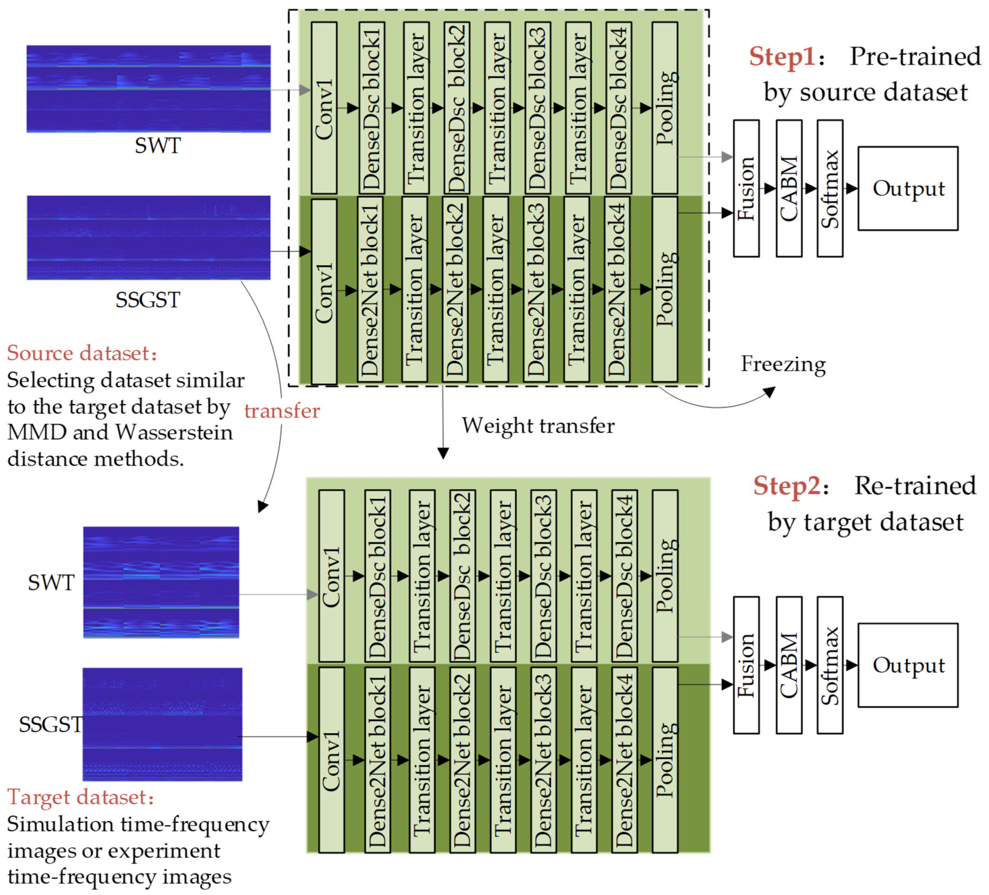
The source data set is automatically selected from the candidate data sets for transfer learning using MMD and Wasserstein distance methods.

(2)

The TSDen2NetRS was trained by the source data set.

Step2: Retraining using the target data set.

(1)

Determining the target data set and its labels.

(2)

Modifying the input data size and output data labels of the network structure according to the target data set.

(3)

The parameters of the original pre-trained network model remain unchanged except for the high-level and full connection layer, and then the target data set is used to retrain the network.

(4)

Finally, the network model is fine-tuned by the target data set.

3. Data Acquisition and Processing

A customized TDG-200/10-0.4 kV three-phase transformer with a frequency of 50 Hz is used for verifying the fault diagnosis method proposed in the current study. The transformer parameters are shown in

Table 2. Transformer parameters.

Name	Value	Name	Value
Transformer model	TDG-200/10-0.4 kV	Link group label	Dyn11
High/low-voltage winding turns	1732/40	High/Low-voltage winding current(A)	11.5/288.7A
High/low-voltage side rated voltage	10/0.4 kV	Impedance voltage/%	4.0
Low-voltage winding outer diameter/(mm)	251 mm	High-voltage winding outer diameter/(mm)	368 mm
Low-voltage winding height/(mm)	403 mm	High-voltage winding height/(mm)	425 mm

. The length of the transformer is 740 mm, the width is 400 mm, and the height is 640 mm. The transformer is a core structure, the high-voltage winding is a cake structure, and the low-voltage winding is a layered structure. When the transformer is abnormal, the vibration signals of the transformer will change accordingly.

3.1. Experiment

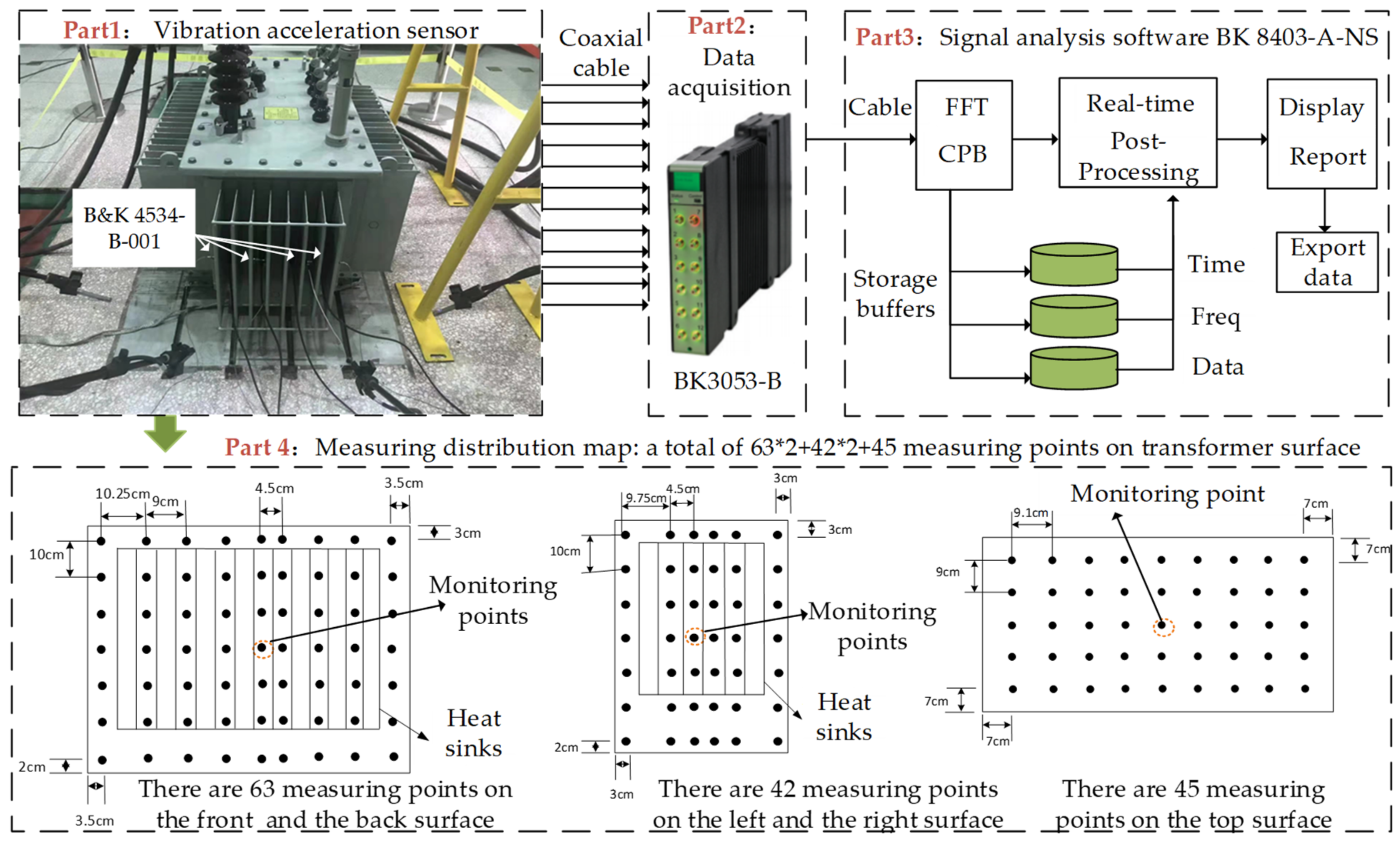
3.1.1. Experiment System

In order to measure the vibration signals of the transformer accurately, a signal acquisition platform is built, as shown in Figure 8, which is composed of vibration acceleration sensors, data acquisition hardware, and signal analysis software. The sensor and acquisition hardware are connected by coaxial cable, and the acquisition hardware and analysis software are connected by wire.

Velocity, displacement, and acceleration sensors can be used for measuring vibration signals. The velocity sensor has high sensitivity but narrow bandwidth. The displacement sensor has poor anti-interference performance for adopting the principle of electromagnetic induction. Acceleration sensors mainly include capacitive, resistive, piezoelectric sensors. The capacitive acceleration sensor works by changing the capacitance pole distance, but its output is nonlinear, the range is limited, and the versatility is not as suitable as the piezoelectric sensor. The resistive acceleration sensor works by resistivity, and its frequency response range is from 2 to 270 Hz, which is not suitable for measuring the vibration signals of the transformer. The piezoelectric acceleration sensor works by the piezoelectric effect. Due to its wide frequency range and high precision, a piezoelectric sensor is selected to measure the vibration signals of the transformer.

Through theoretical analysis and experimental measurement, the maximum amplitude of transformer vibration under short-circuit impact is ±15 g, and the frequency distribution is within 1 kHz. In this case, the B & K4534-001 piezoelectric acceleration sensor is selected finally because its measuring range is ±71 g, and the frequency response range is from 0.2 to 12.8 kHz, which is higher than the vibration amplitude and frequency of the transformer. The precision of the sensor is 0.00013 g. Each unit of the B & K4534-001 sensor has a lightweight, robust, hermetically sealed titanium housing and an insulated base, which makes the sensor suitable for use in tough environments. In general, through the analysis above, we can conclude that the B & K4534-001 sensor is suitable for transformer vibration experiments.

The 3053 LAN-XI data acquisition hardware is selected to simultaneously acquire 12-channel signals. The frequency range is from 0 to 25.6 kHz. Meanwhile, the sampling rate is set at 8192 Hz, each sampling time is 10 s, and the sampling interval is 30 mins.

The signal analysis software is LabShop, which can display, store and analyze vibration signals.

The measurement points are evenly arranged on each surface of the transformer, as shown in Figure 8, including 63 points on the front and back surfaces of the transformer, 42 points on the left and right surfaces of the transformer, and 45 points on the top surface of the transformer.

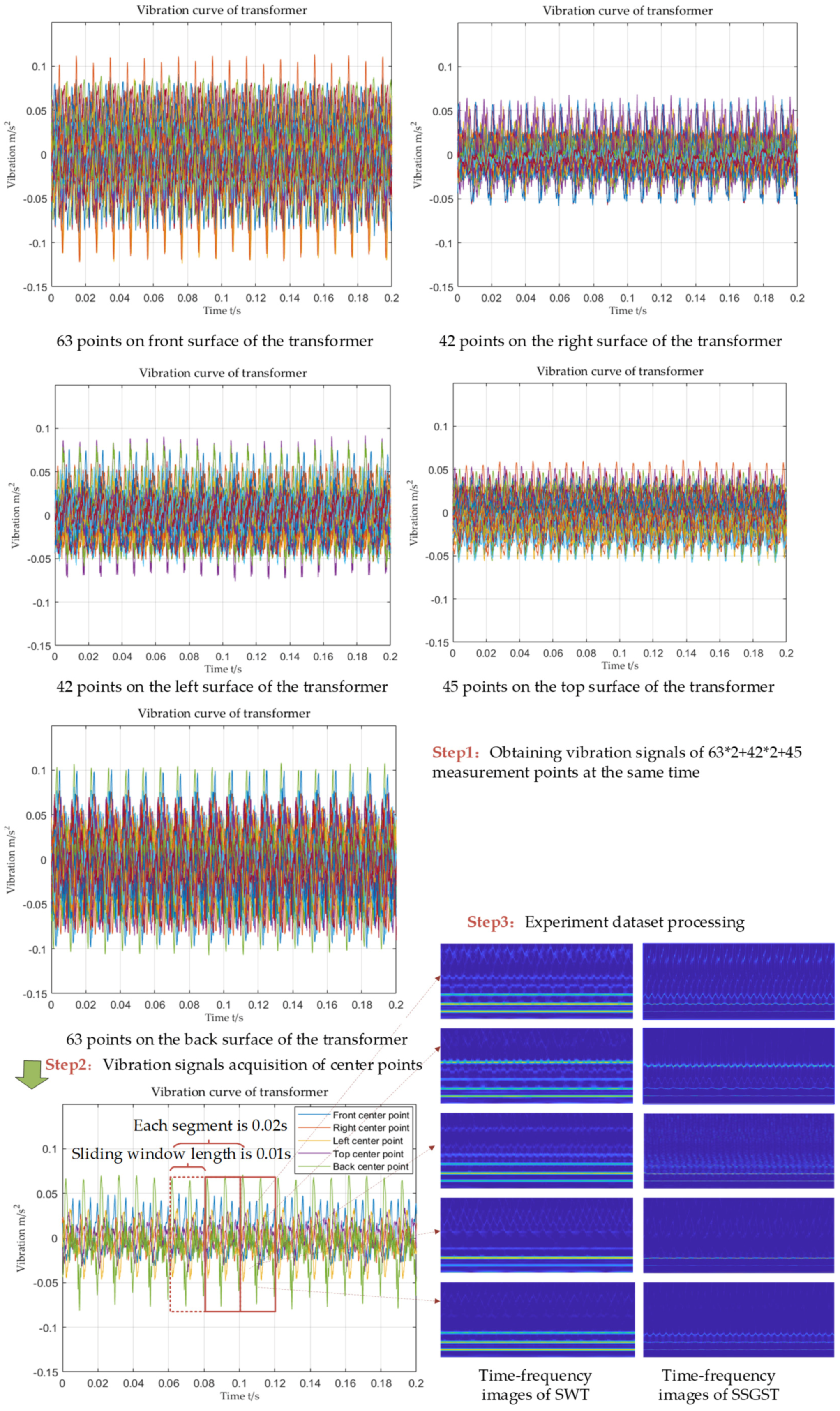
3.1.2. Experimental Data Set Acquisition and Processing

As shown in Figure 9, the time-domain signals can be obtained from different measuring points. The results indicate that the vibration signals of each point are different. After comparison and analysis of multiple points, the center points of each surface are finally selected as the monitoring points for different operating states of the transformer.

The transformer faults mainly include insulation shedding, winding looseness, and deformation. The labels are represented by $L_{\xi }=\left\{0, 1, 2, 3\right\}$, and the number of labels is 4, and the normal state is ‘0′. In order to obtain fault vibration signals with different fault types, severities, and locations, a customized transformer with fault winding is used for replacing normal transformers. The specific process is as follows: first, the insulation shedding fault is realized by changing the connection components between winding turns. A Mini Circuit Breaker (MCB) is employed to control the connection of the variable resistor between the two turns. Second, the looseness fault is realized by the customized transformer with loose windings. Third, the deformation fault is realized by customizing the transformer with deformation windings.

The sliding window method divides the vibration signals into 0.02 s time series segments. The 40 sample points are selected from the segments, which are transformed into time-frequency images by the SWT and SSGST combined methods. The detailed process is shown in Figure 9.

The amount and labels of the experimental data set are provided in

Table 3. Transformer vibration data set.

Type	Label	Data Set		SWT/SSGST Time-Frequency Images
		Simulation	Experiment	Simulation	Experiment
Normal	0	3000	300	3000	300
Insulation shedding	1	3400	300	3400	300
Looseness	2	3000	300	3000	300
Deformation	3	3600	300	3600	300
Total number	-	13,000	1200	13,000	1200

.

3.2. Simulation

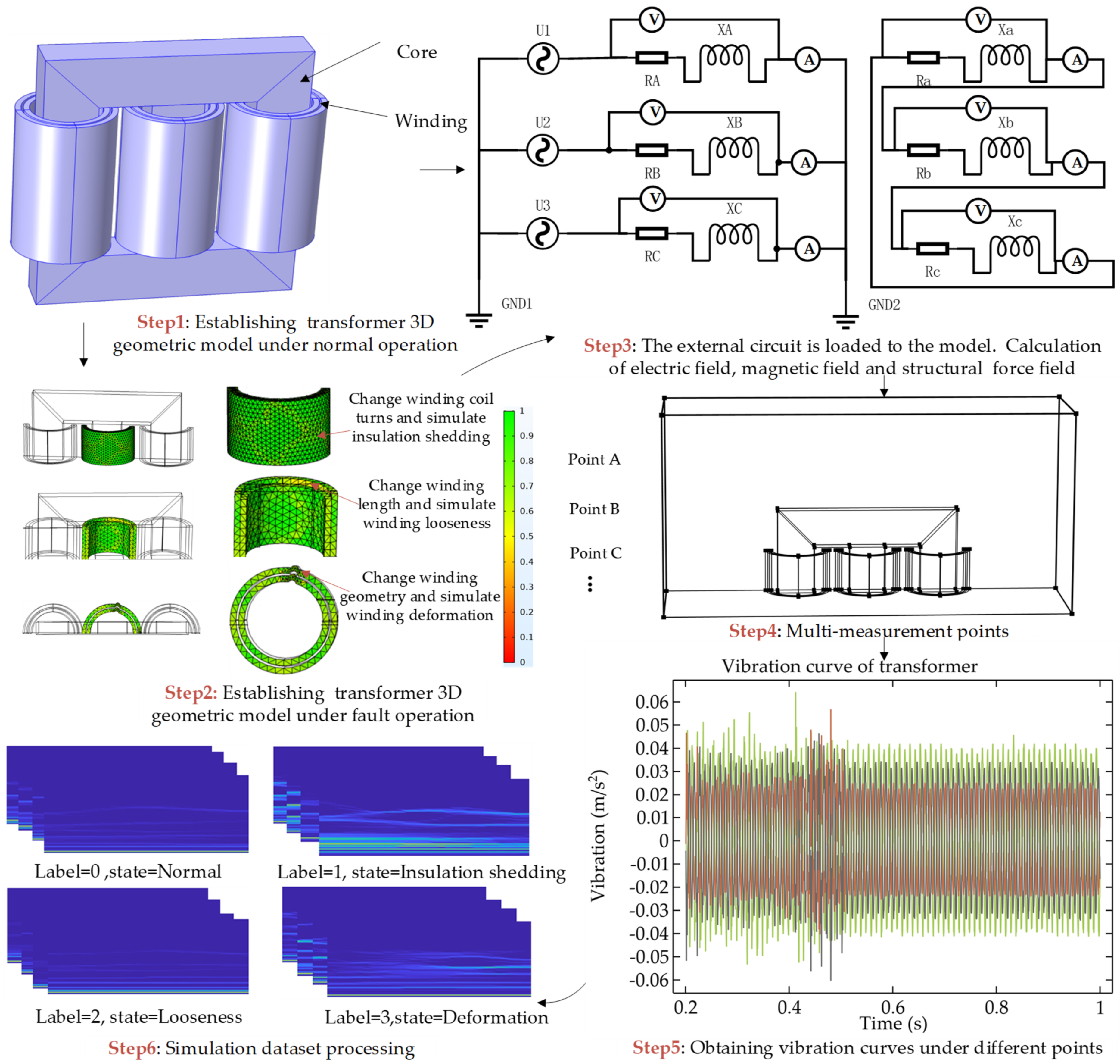
3.2.1. Simulation Model Establishment

The amount and labels of the simulation data set are shown in Table 3. The specific procedures for obtaining the transformer vibration simulation data set are shown in Figure 10.

The simulation model is established using COMSOL finite element software [38,39,40,41,42,43], which performs a multifield coupling calculation of the external circuit, magnetic field, and structural force field.

Establishing a three-dimensional geometric model of the transformer, according to the actual size of the iron core and three-phase windings. However, in order to reduce the computation, a quarter of the simplified transformer model is used.

Performing multi-physics coupling model.

(1)

The iron core material is silicon steel sheet, and the winding material is copper. In the electromagnetic field, the external circuit is loaded into the electric field model through the field-circuit coupling method. The control equation in the electric field can be established using the following formula

$$-\nabla \times \frac{\partial \left({\epsilon }_0{\epsilon }_r\right)\nabla V}{{\partial }_t}-\nabla ·\left(\sigma \nabla V-J^e\right)=0$$

(12)

where$\nabla \times$ is curl operator, $\nabla ·$ is divergence operator; ${\epsilon }_0$ is the vacuum dielectric constant of the free space; ${\epsilon }_r$ is the relative dielectric constant; $V$ is the potential;$\sigma$ is the conductivity; $J^e$ is the external current density.

(2)

Establishing an electromagnetic field coupling model. The external current density $J^e$ is calculated in the electric field, and then it serves as an excitation of the magnetic field, which can be expressed as

$$\sigma \frac{\partial A}{\partial t}+\nabla \times \left({\mu }_0^{-1}{\mu }_r^{-1}\nabla \times A\right)=J^e$$

(13)

where $\nabla \times$ is the curl operator; $A$ is the magnetic vector potential;${\mu }_0$ is the magnetic permeability; and${\mu }_r$ is the relative magnetic permeability.

(3)

Realizing the coupling of the electromagnetic field and the structural force field. The current density, magnetic flux density, and magnetic field strength are calculated in the electromagnetic field, and then these variables are used in the structural force field. Thus, physical quantities, including winding vibration acceleration, velocity, and displacement, are calculated.

Electromagnetic force $F\left(t\right)$ is decomposed into three directions, representing three-dimensional space. The formula is as follows

$$\left\{\begin{array}{c}{F}_x=J_y{B}_z-J_z{B}_y\\ F_y=J_z{B}_x-J_x{B}_z\\ F_z=J_x{B}_y-J_y{B}_x\end{array}\right.$$

(14)

where $F_x,F_y,F_z$ represent electromagnetic forces in x, y, z directions; $J_x$, $J_y$, $J_z$ represent current density in x, y, z directions; $B_x$, $B_y$, $B_z$ represent magnetic flux densities in x, y, z directions.

The control equation in the structural field can be described as

$$M\frac{d^{2}S}{d{t}^2}+\varsigma \frac{dS}{dt}+GS=F\left(t\right)$$

(15)

where $M$ is the mass matrix; $\frac{d^{2}S}{d{t}^2}$is the winding acceleration; $\frac{dS}{dt}$ is the winding speed;$\varsigma$ is the damping coefficient matrix; $G$is the stiffness matrix;$S$ is the winding displacement; and$F\left(t\right)$ is the electromagnetic force on the winding.

3.2.2. Simulation Data Set Acquisition and Processing

In this study, three types of transformer fault models are established by COMSOL simulation software, which mainly includes winding insulation shedding, winding looseness, and deformation.

The insulation shedding simulation model is established by reducing the original number of turns from 5% to 20%.

The looseness fault simulation model is established by changing the original axial winding length from 5% to 20%.

The deformation fault simulation model is established by changing the surface area of the winding at 1/2 position from 10% to 20%.

The simulation vibration acceleration signals are obtained through point diagrams at different locations of the transformer by COMSOL software, and then these signals are transformed into time-frequency images by the sliding window and time-frequency methods.

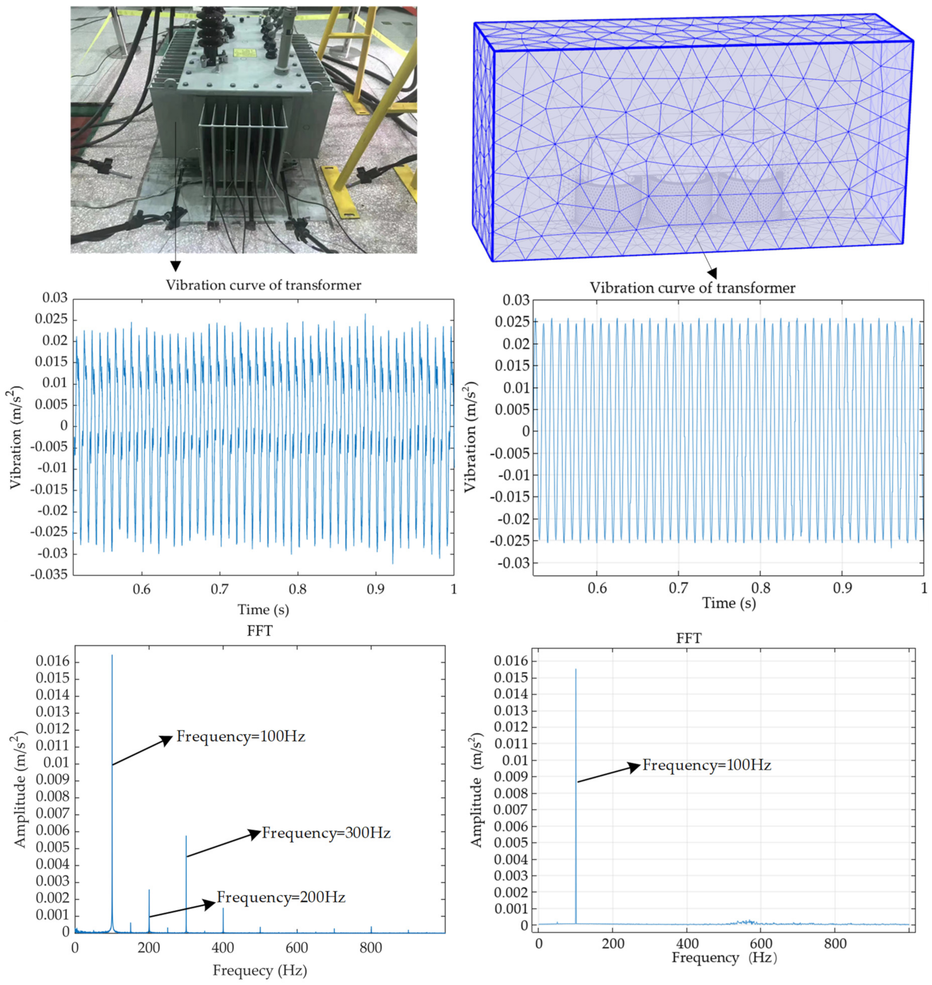
3.3. Simulation and Experimental Data Analysis

To verify the accuracy and rationality of the simulation model, a comparative test with experimental signals is conducted.

The similarity between experimental and simulation signals is calculated by the 2D correlation coefficient (corr2) function, which can be calculated as

$$corr2=\frac{{{\displaystyle \sum }}_{Line}{{\displaystyle \sum }}_{Col}\left(E_{LineCol}-\overline{E}\right)}{\sqrt{\left({{\displaystyle \sum }}_{Line}{{\displaystyle \sum }}_{Col}{\left(D_{LineCol}-\overline{D}\right)}^2\right)\left({{\displaystyle \sum }}_{Line}{{\displaystyle \sum }}_{Col}{\left(E_{LineCol}-\overline{E}\right)}^2\right)}}$$

(16)

where $corr2$ is the 2-D correlation coefficient. $D$ and $E$ depict vibration signal mapping data matrices of the experiment and simulation; $Line$ and $Col$ represented the number of lines and columns in the matrices, respectively.

The experimental and simulation vibration signal curves under the rated load are shown in Figure 11. The similarity calculated by corr2 is 0.9712, which proves the accuracy of the simulation model.

As for the difference of the frequency domain, the experimental signal contains high-frequency information of 200–500 Hz in addition to the fundamental frequency of 100 Hz. This is due to the uneven distribution of insulation between the actual transformer winding turns. By comparing the experimental and simulation signals, the amplitude is about 0.016 m/s² at the fundamental frequency of 100 Hz, which verifies the correctness of the fundamental frequency vibration of the simulation model.

4. Results and Comparisons

To verify the accuracy and robustness of the proposed method, the performance of the method is tested under different time-frequency methods and interferences.

4.1. SWT and SSGST Combined Time-Frequency Analysis Method

4.1.1. Time-Frequency Analysis Results

The SWT and SSGST time-frequency analysis (TFA) methods improve the energy concentration compared with the traditional time-frequency methods, including STFT, CWT, and GST. The results are presented in Figure 12.

Furthermore, in order to evaluate the energy concentration of the different time-frequency methods quantitatively, we calculate the Rényi entropies as listed in

Table 4. Rényi entropies by five TFA methods.

TFA	STFT	CWT	GST	SWT	SSGST
Rényi entropies	19.6057	16.3274	16.1428	15.3513	12.5701

.

The results indicate that the energy of SWT and SSGST time-frequency analysis methods is more concentrated and more sensitive to the changes of time-frequency images.

4.1.2. Comparison of Diagnosis Performance with Different Time-Frequency Analysis Methods

To prove the superiority of the time-frequency methods in fault diagnosis, the paper compares the SWT and SSGST time-frequency methods with the method based on one-dimensional data. The results are shown in line 1) of

Table 5. Deep fault diagnosis of different methods.

Type	Method	Test Accuracy (Simulation Data Set)	Test Accuracy (Experimental Data Set)
(1) (with one-dimensional vibration data)	One-dimensional data	94.11% (960/1020)	88.33% (106/120)
(2) (with single visualization feature extraction)	STFT	91.47% (933/1020)	89.16% (107/120)
	CWT	92.94% (948/1020)	88.33% (106/120)
	GST	96.08% (980/1020)	87.50% (105/120)
	SWT	96.18% (981/1020)	90.83% (109/120)
	SSGST	96.57% (985/1020)	90.83% (109/120)
(3) (with combined visualization feature extraction)	SWT+ SSGST	97.25% (992/1020)	95.00% (114/120)

. The accuracy based on one-dimensional data in the simulation data set is 94.11%, which is 2.07% and 2.46% lower than the SWT and SSGST methods. The accuracy in the experimental data set is 88.33%, which is 2.5% lower than the SWT and SSGST methods.

In order to better verify the effectiveness of the SWT and SSGST time-frequency methods, they are compared with other time-frequency analysis methods. The final results are shown in line 2) of Table 5. The accuracy of SWT and SSGST in the simulation data set is higher than that of the other three time-frequency methods, reaching 96.18% and 96.57%. The accuracy of SWT and SSGST in the experimental data set is 90.83%, which is 2.5% higher than that of other time-frequency methods on average.

To further highlight the importance of the combined time-frequency method, the SWT and SSGST combined method is compared with other methods. The results in line (3) of Table 5 show that the method achieves the best classification performance, reaching 97.25% and 95%.

Consequently, the SWT and SSGST combined time-frequency analysis method has a great influence on the accuracy of fault diagnosis.

4.2. TSDen2NetRS Method

4.2.1. Comparison of Diagnosis Performance with Different Intelligent Diagnosis Methods

In order to verify the advantages of the proposed deep learning fault diagnosis method, this paper compares it with different intelligent classification methods, including SVM and K-Nearest Neighbor (KNN) [20]. The different intelligent methods are trained by simulation and experimental data sets obtained by SSGST. The results are shown in Table 7. The accuracy of the proposed method in the experimental data set and the simulation data set is higher than that of the other two intelligent methods, reaching 95% and 97.25%, which are 9.3% and 19.3% higher than that of the SVM and KNN methods on average.

In order to further illustrate the high-precision fault diagnosis of the proposed TSDen2NetRS method, this paper compares it with other deep learning methods, including Xception [44], ResNet50 [29], InceptionV3 [45], MobileNet [46], and DenseNet121 [30]. The hyperparameters of different deep learning methods are set in

Table 6. Hyperparameter settings.

Type	Setting
Initial learning rate	0.001
Learning rate schedule	piecewise
Mini batch size	32
Max epochs	20
Learning rate drop period	25
Learning rate drop factor	0.2
Execution environment	GPU
Optimizer	Adam
Verbose	0

. Meanwhile, the simulation and experimental data sets are divided into training, validation, and testing data sets in accordance with the ratio of 7:2:1. The accuracy of the fault diagnosis results of different deep learning methods is shown in line 2) of

Table 7. Results of different intelligent fault diagnosis methods.

Type	Method	Test Accuracy (Simulation Data Set)	Test Accuracy (Experimental Data Set)
(1) Traditional intelligent classification method	SVM	65.10% (664/1020)	84.17% (101/120)
	KNN	90.69% (925/1020)	88.33% (106/120)
(2) Deep learning method (CNNS)	Xception	96.56% (985/1020)	90.83% (109/120)
	ResNet50	91.17% (930/1020)	81.67% (95/120)
	InceptionV3	93.33% (952/1020)	91.67% (110/120)
	MobileNet	93.53% (954/1020)	92.50% (111/120)
	DenseNet121	91.67% (935/1020)	89.17% (107/120)
	TSDen2NetRS	97.25% (992/1020)	95.00% (114/120)

. The results indicate that the accuracy of the proposed method in the experimental data set and the simulation data set reaches 95% and 97.25%, which is improved by 5.8% and 3.8% on average.

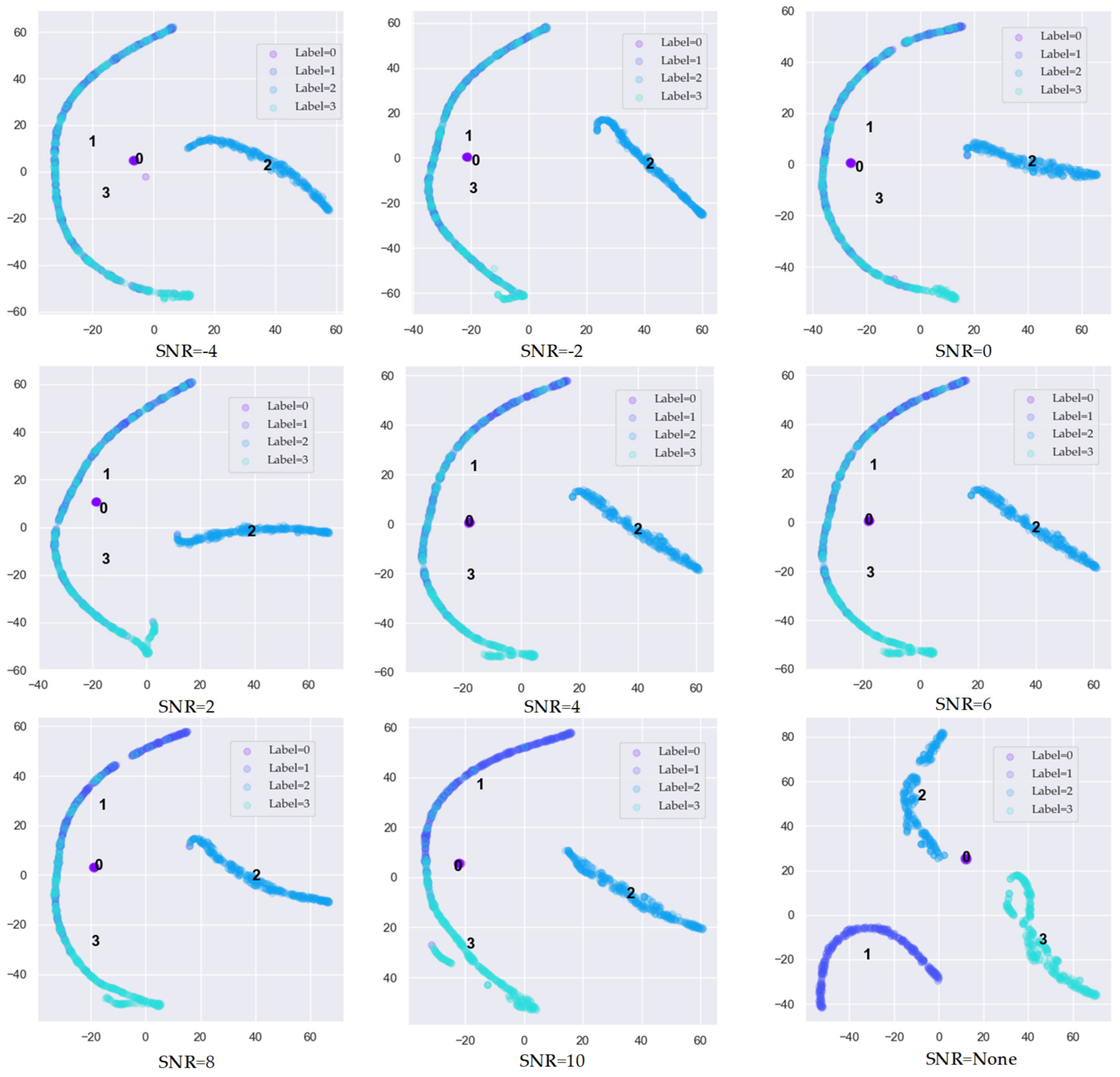
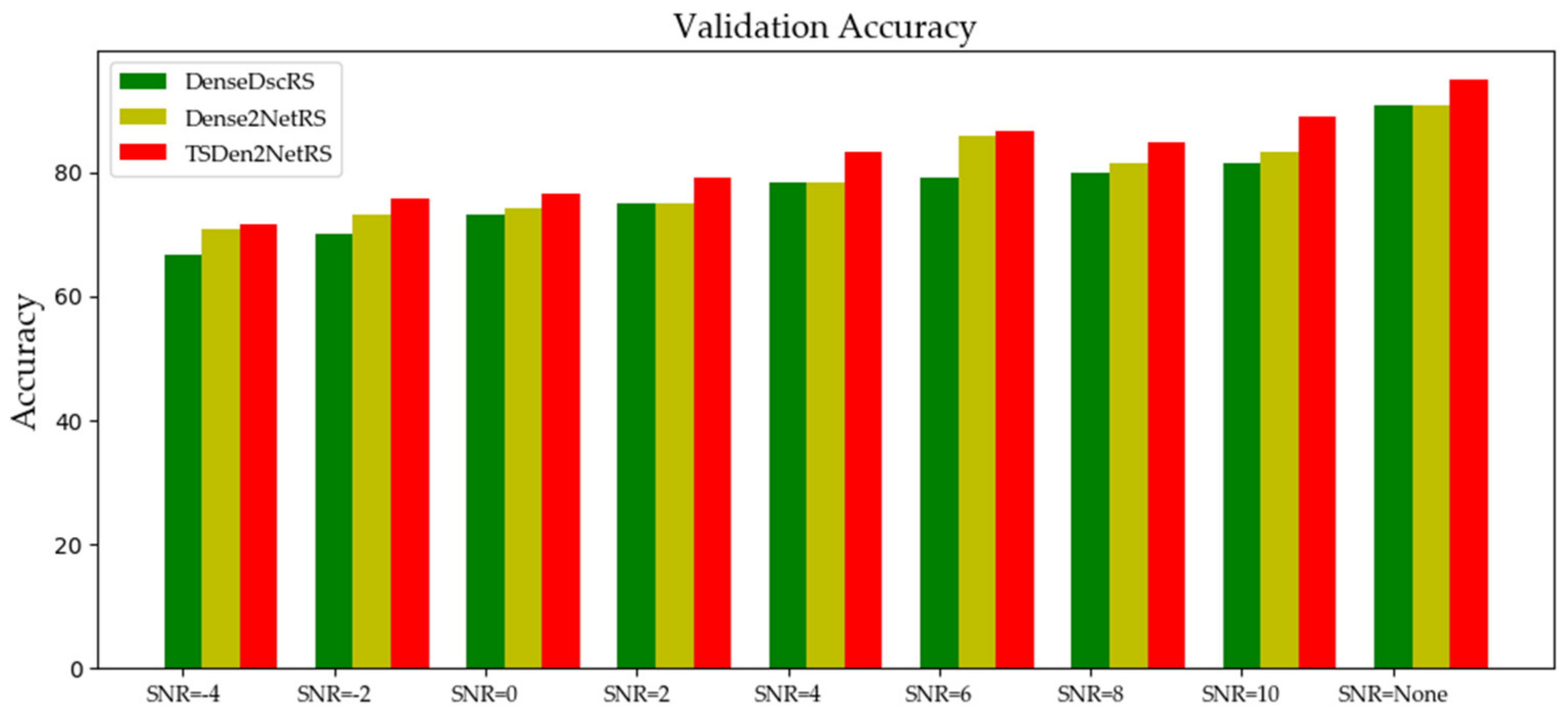
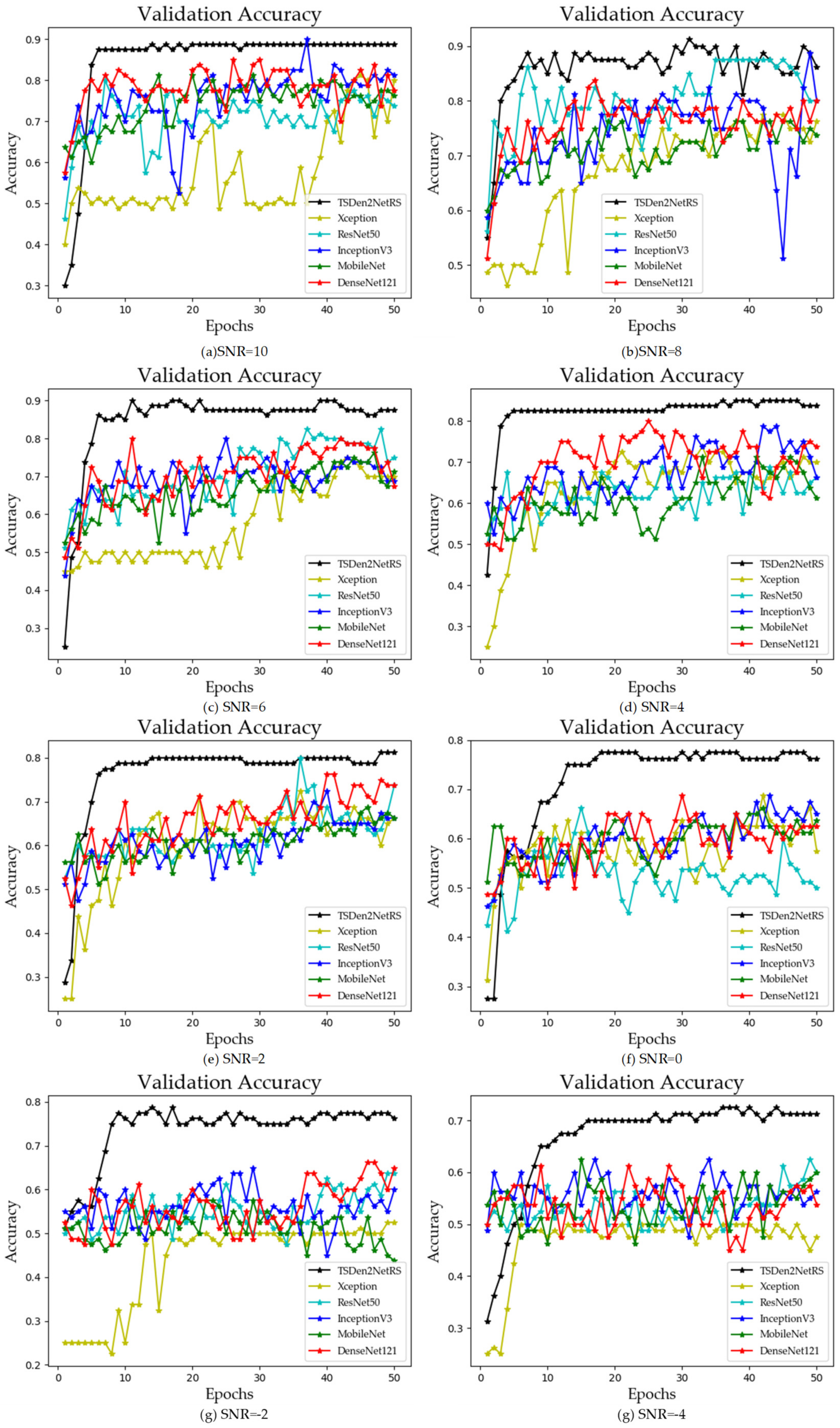
4.2.2. Comparison of Anti-Interference with Different Intelligent Diagnosis Methods

In order to test the anti-interference performance of the proposed method, Gaussian noise is applied to the original data to evaluate the diagnostic performance of the model in different interference environments. Signal-to-Noise Ratio (SNR) is adopted in the current study, and the formula is defined as follows

$$SNRdB=10lo{g}_{10}\left(P_{signal}/P_{noise}\right)$$

(17)

where $P_{signal}$ represents the original signal; $P_{noise}$ represents the additional Gaussian noise.

The fault classification performance after the addition of different noise interferences to the original signals is presented in Figure 13. The results show that different types of faults are gradually separated with a decrease in noise interference. Meanwhile, signals at the same label become closer, and the labels of different types become sparser. Therefore, signal noise interference seriously affects the diagnostic performance, and research on the anti-interference performance of the method is necessary. The experimental data set is used as the input of the deep learning network.

The accuracy of the TSDen2NetRS method is compared with that of single-stream Dense2NetRS and DenseDscRS methods. The results in Figure 14 show that the two-stream method has better diagnostic performance than single-stream methods under different interferences.

In addition, the anti-interference performance of TSDen2NetRS is compared with that of the Xception, ResNet50, InceptionV3, MobileNet and DenseNet121 methods. The results are presented in Figure 15. When the SNR is 10, 8, 6, 4, 2, 0, −2, −4, the TSDen2NetRS method exhibits better anti-interference performance, with the accuracy of 89.16%, 85.00%, 86.66%, 83.33%, 79.16%, 76.66%, 75.83%, 71.66%, which is 11.86%, 8.8%, 15.66%, 14.33%, 16.9%, 16.41%, 19.35%, 15.66% higher than that of other methods on average.

4.3. Adaptive Transfer Learning Method between Different Domains

Compared with the traditional transfer learning methods [36,37], the adaptive method can automatically select the source domain by using the domain measurement method. In order to prove the advantages of the proposed method, the experiments are designed to contain eight cases in

Table 8. Adaptive transfer learning results between different domains.

Network	Domain	MMD	WD	$\widehat{\mathit{d}}$	Transfer Accuracy
(1) Single- stream (Dense2NetRS)	ImageNet-Simulation	0.8379	108.79	1.9174	96.96% (989/1020)
	Fusion-Simulation	0.6937	20.09	0.8877	97.64% (996/1020)
	Stitching-Simulation	0.7973	57.48	1.3641	97.45% (994/1020)
	ImageNet-Experiment	0.7868	112.85	1.9074	91.67% (110/120)
	Fusion-Experiment	0.5760	20.75	0.7777	92.50% (111/120)
	Stitching-Experiment	0.7173	60.27	1.3128	91.67% (110/120)
	Simulation-Experiment	0.4915	8.65	0.5731	95.83% (115/120)
(2) Two-stream (TSDen2NetRS)	Simulation-Experiment	0.4915	8.65	0.5731	98.33% (118/120)

. In each case, the source data set is one of the candidate data sets, and the target data set is the simulation data set or experimental data set.

In this paper, four data sets are selected as candidate data sets, which mainly include:

(1)

ImageNet data set: the public data set;

(2)

Fusion data set: ImageNet is extracted with the same size, type, and number as the SWT or SSGST time-frequency images and then fusing them;

(3)

Stitching data set: ImageNet is extracted with the same size, type, and number as the SWT or SSGST time-frequency images and then stitches them;

(4)

Simulation data set: The time-frequency images of the simulation data set generated by COMSOL software.

The transfer learning results between different data sets are shown in Table 8.

(1)

The network structure is Dense2NetRS signal-stream. The first three lines indicate that when the target data set is the simulation data set, the smaller the value of $\widehat{d}$ is, the higher the accuracy of the transfer learning is. The results from the fourth to seventh lines show that when the target data set is the experimental data set, the smaller the value of $\widehat{d}$ is, the better the performance of the transfer learning is, which verifies the feasibility of adaptive source data set selection through the domain measurement method. Further, the accuracy in the seventh line of fault diagnosis can be increased from 90.83% to 95.83%.

(2)

The network structure is TSDen2NetRS two-stream. The accuracy in the last line of Table 8 increased from 95.00% to 98.33%. The result proves that the adaptive transfer learning method applied to a two-stream network can achieve higher diagnostic accuracy.

Moreover, as the results show in Figure 16, it can be clearly noticed that the proposed adaptive transfer learning method based on the TSDen2NetRS network can achieve the best accuracy in different cases. This can effectively prove the feasibility of the proposed method and its superiority in fault diagnosis.

5. Conclusions

An adaptive transfer learning method based on a two-stream densely connected residual shrinkage network for transformer fault diagnosis is proposed in this paper. For the experimental data set, the fault diagnosis accuracy of TSDens2NetRS based on the SWT and SSGST combined method can reach 95%. Compared with other intelligent diagnostic methods, the accuracy of the proposed method is 9.3% higher than other methods on average. Meanwhile, for anti-interference performance, the diagnosis accuracy of the proposed method is 15.66% higher than other deep learning methods on average when the SNR is -4. In addition, the final accuracy of TSDen2NetRS with the adaptive transfer learning method increases from 95% to 98.33%, which means the proposed method has better fault diagnosis performance. The conclusions of this study are as follows:

(1)

The results of the time-frequency methods show that the SWT and SSGST combined method can extract more concentrated energy signals, which can better reflect the changes of the signals than the traditional time-frequency methods.

(2)

The TSDen2NetRS method results show that the novel method can effectively distinguish different transformer faults in a strong interference environment and greatly improve fault diagnosis accuracy.

(3)

The results of the adaptive transfer learning method show that it can automatically select the source domain, which has the closest distribution to the target domain. Moreover, it can greatly improve the diagnosis performance under small samples.

In our future work, the diagnostic performance of the proposed method on variable working conditions and complex industrial scenes will be further investigated.

References

1. Wu, Z.; Zhou, L.; Lin, T.; Zhou, X. A New Testing Method for the Diagnosis Winding Faults in Transformer. IEEE Trans. Instrum. Meas. 2016, 69, 9203–9214. [Google Scholar] [CrossRef]
2. Wang, S.; Wang, S.; Zhang, N.; Yuan, D.; Qiu, H. Calculation and analysis of mechanical characteristics of transformer windings under short-circuit condition. IEEE Trans. Magn. 2019, 55, 1–4. [Google Scholar] [CrossRef]
3. Bagheri, S.; Moravej, Z.; Gharehpetian, G. Classification and discrimination among winding mechanical defects, internal and external electrical faults, and inrush current of transformer. IEEE Trans. Ind. Informat. 2018, 14, 484–493. [Google Scholar] [CrossRef]
4. Khan, S.; Equbal, M.; Islam, T. A comprehensive comparative study of DGA based transformer fault diagnosis using fuzzy logic and ANFIS models. IEEE Trans. Dielectr. Elect. Insul. 2015, 22, 590–596. [Google Scholar] [CrossRef]
5. Liu, Y.; Ji, S.; Yang, F.; Cui, Y.; Zhu, L.; Rao, Z.; Ke, C.; Yang, X. A study of the sweep frequency impedance method and its application in the detection of internal winding short circuit faults in power transformers. IEEE Trans. Dielectr. Electr. Insul. 2015, 22, 2046–2056. [Google Scholar] [CrossRef]
6. Li, Y.; Yan, X.; Wang, C.; Yang, Q. Eddy Current Loss Effect in Foil Winding of Transformer Based on Magneto-Fluid-Thermal Simulation. IEEE Trans. Magn. 2019, 55, 1–5. [Google Scholar] [CrossRef]
7. Soleimanni, M.; Faiz, J.; Nasab, P.; Moallem, M. Temperature Measuring-Based Decision-Making Prognostic Approach in Electric Power Transformers Winding Failures. IEEE Trans. Instrum. Meas. 2020, 69, 6995–7003. [Google Scholar] [CrossRef]
8. Kim, J.; Park, B.; Jeong, S.; Kim, S.; Park, P. Fault diagnosis of a Power Transformer Using an Improved Frequency-Response Analysis. IEEE Trans. Power Del. 2005, 20, 169–177. [Google Scholar] [CrossRef]
9. Duan, J.; He, Y.; Wu, W. Fault localization on transformer winding by frequency response analysis and evidential reasoning. J. Eng. 2019, 2019, 9079–9082. [Google Scholar] [CrossRef]
10. Hu, Y.; Zheng, J.; Huang, H. Experimental Research on Power Transformer Vibration Distribution under Different Winding Defect Conditions. Electronics 2019, 8, 842–861. [Google Scholar] [CrossRef] [Green Version]
11. Bhide, R.; Srinivas, M.; Banerjee, A.; Somakumar, R. Analysis of Winding Inter-Turn Fault in Transformer: A Review and Transformer Models. In Proceedings of the 2010 IEEE International Conference on Sustainable Energy Technologies, Kandy, Sri Lanka, 6–9 December 2010; pp. 1–7. [Google Scholar]
12. Hong, K.; Huang, H.; Fu, Y.; Zhou, J. A vibration measurement system for health monitoring of power transformers. Measurement 2016, 93, 135–147. [Google Scholar] [CrossRef]
13. Wu, S.; Huang, W.; Kong, F.; Wu, Q.; Zhou, F.; Zhang, R.; Wang, Z. Extracting power transformer vibration features by a time-scale-frequency analysis method. J. Electromagn. Anal. Appl. 2010, 2, 31–38. [Google Scholar] [CrossRef] [Green Version]
14. Guo, M.; Yang, N.; Chen, W. Deep-learning-based fault classification using Hilbert-Huang transform and convolutional neural network in power distribution system. IEEE Sens. J. 2010, 19, 6905–6913. [Google Scholar] [CrossRef]
15. Xu, Y.; Zhao, C.; Xie, S.; Lu, M. Novel Fault Location for High Permeability Active Distribution Networks Based on Improved VMD and S-transform. IEEE Access 2021, 9, 17662–17671. [Google Scholar] [CrossRef]
16. Shao, S.; McAleer, S.; Yan, R.; Baldi, P. Highly Accurate Machine Fault Diagnosis Using Deep Transfer Learning. IEEE Trans. Ind. Inform. 2019, 15, 2446–2455. [Google Scholar] [CrossRef]
17. Daubechies, I.; Lu, J.; Wu, H. Synchrosqueezed wavelet transforms: An empirical mode decomposition-like tool. Appl. Comput. Harmon. Anal. 2011, 30, 243–261. [Google Scholar] [CrossRef] [Green Version]
18. Auger, F.; Flandrin, P.; Lin, Y.; McLaughlin, S.; Meignen, S.; Oberlin, T.; Wu, H. Time-Frequency Reassignment and Synchrosqueezing: An Overview. IEEE Signal Process. Mag. 2013, 30, 32–41. [Google Scholar] [CrossRef] [Green Version]
19. Wang, Q.; Gao, J.; Liu, N.; Jiang, X. High-Resolution Seismic Time-Frequency Analysis Using the Synchrosqueezing Generalized S-Transform. IEEE Geosci. Remote Sens. Lett. 2018, 15, 374–378. [Google Scholar] [CrossRef]
20. Zhang, H.; Berg, A.; Maire, M.; Malik, J. SVM-KNN: Discriminative Nearest Neighbor Classification for Visual Category Recognition. In Proceedings of the 2006 IEEE Computer Society Conference on Computer Vision and Pattern Recognition (CVPR’06), New York, NY, USA, 17–22 June 2006; Volume 2, pp. 2126–2136. [Google Scholar]
21. Zhao, C.; He, Y.; Jiang, S.; Wang, T.; Yuan, L.; Li, B. Transformer Fault Diagnosis Method Based on Self-Powered RFID Sensor Tag, DBN, and MKSVM. IEEE Sens. J. 2019, 19, 8202–8212. [Google Scholar]
22. Wang, T.; He, Y.; Shi, T.; Li, B. Transformer Health Management Based on Self-Powered RFID Sensor and Multiple Kernel RVM. IEEE Trans. Instrum. Meas. 2019, 68, 818–828. [Google Scholar] [CrossRef]
23. Hinton, G.; Osindero, E.; Teh, Y. A fast learning algorithm for deep belief nets. Neural Comput. 2006, 18, 1527–1554. [Google Scholar] [CrossRef] [PubMed]
24. Wen, L.; Gao, L.; Li; X. A New Deep Transfer Learning Based on Sparse Auto-Encoder for Fault Diagnosis. IEEE Trans. Syst. Man Cybern. 2017, 49, 136–144. [Google Scholar] [CrossRef]
25. Wen, L.; Li, X.; Gao, L.; Zhang, Y. A new convolutional neural network-based data-driven fault diagnosis method. IEEE Trans. Ind. Electron. 2018, 65, 5990–5998. [Google Scholar] [CrossRef]
26. Ince, T.; Kiranyaz, S.; Eren, L.; Askar, M.; Gabbouj, M. Real-time motor fault detection by 1-D convolutional neural networks. IEEE Trans. Ind. Electron. 2016, 63, 7067–7075. [Google Scholar] [CrossRef]
27. Chen, C.; Liu, Z.; Yang, G.; Wu, C.; Ye, Q. An Improved Fault Diagnosis Using 1D-Convolutional Neural Network Model. Electronics 2021, 10, 59–78. [Google Scholar] [CrossRef]
28. Liu, R.; Wang, F.; Yang, B.; Qin, S. Multiscale Kernel Based Residual Convolutional Neural Network for Motor Fault Diagnosis under Nonstationary Conditions. IEEE Trans. Ind. Inform. 2020, 16, 3797–3806. [Google Scholar] [CrossRef]
29. Zhao, M.; Zhong, S.; Fu, X.; Tang, B.; Pecht, M. Deep Residual Shrinkage Networks for Fault diagnosis. IEEE Trans. Ind. Inform. 2020, 16, 4681–4690. [Google Scholar] [CrossRef]
30. Huang, G.; Liu, Z.; Van Der Maaten, L.; Weinberger, K. Densely Connected Convolutional Networks. In Proceedings of the IEEE Conference on Computer Vision and Pattern Recognition, Honolulu, HI, USA, 21–26 July 2017; pp. 4700–4708. [Google Scholar]
31. Li, G.; Zhang, M.; Li, J.; Lu, F.; Tong, G. Efficient densely connected convolutional neural networks. Pattern Recognit. 2021, 109, 107610. [Google Scholar] [CrossRef]
32. Miao, M.; Liu, C.; Yu, J. Adaptive Densely Connected Convolutional Auto-Encoder-Based Feature Learning of Gearbox Vibration Signals. IEEE Trans. Instrum. Meas. 2021, 70, 1–11. [Google Scholar]
33. Zhou, W.; Chen, Y.; Liu, C.; Yu, L. GFNet: Gate Fusion Network with Res2Net for Detecting Salient Objects in RGB-D Images. IEEE Signal Process. Lett. 2020, 27, 800–804. [Google Scholar] [CrossRef]
34. Gao, S.; Cheng, M.; Zhao, K.; Zhang, X.; Yang, M.; Torr, P.H.S. Res2net: A new multi-scale backbone architecture. IEEE Trans. Pattern Anal. Mach. Intell. 2021, 43, 652–662. [Google Scholar] [CrossRef] [Green Version]
35. He, W.; He, Y.; Li, B. Generative Adversarial Networks with Comprehensive Wavelet Feature for Fault Diagnosis of Analog Circuits. IEEE Trans. Instrum. Meas. 2020, 69, 6640–6650. [Google Scholar] [CrossRef]
36. Chen, Z.; He, G.; Li, J.; Liao, Y.; Gryllias, K.; Li, W. Domain Adversarial Transfer Network for Cross-Domain Fault Diagnosis of Rotary Machinery. IEEE Trans. Instrum. Meas. 2020, 69, 8702–8712. [Google Scholar] [CrossRef]
37. Liu, J.; Ren, Y. A General Transfer Framework based on Industrial Process Fault Diagnosis under Small Samples. IEEE Trans. Ind. Inform. 2020, 17, 6073–6083. [Google Scholar] [CrossRef]
38. Geißler, D.; Leibfried, T. Short-Circuit Strength of Power Transformer Windings-Verification of Tests by a Finite Element Analysis-Based Model. IEEE Trans. Power. Del. 2017, 32, 1705–1712. [Google Scholar]
39. Liu, S.; Liu, Y.; Li, H.; Lin, F. Diagnosis of transformer winding faults based on FEM simulation and on-site experiments. IEEE Trans. Dielectr. Electr. Insul. 2016, 23, 3752–3760. [Google Scholar] [CrossRef]
40. Zhang, H.; Yang, B.; Xu, W.; Wang, S.; Wang, G.; Huangfu, Y.; Zhang, J. Dynamic Deformation Analysis of Power Transformer Windings in Short-Circuit Fault by FEM. IEEE Trans. Appl. Sup. 2013, 24, 1–4. [Google Scholar] [CrossRef]
41. Deng, L.; Sun, Q.; Jiang, F.; Wang, S.; Jiang, S.; Xiao, H.; Peng, T. Modeling and Analysis of Parasitic Capacitance of Secondary Winding in High-Frequency High-Voltage Transformer Using Finite-Element Method. IEEE Trans. Appl. Sup. 2018, 28, 1–5. [Google Scholar] [CrossRef]
42. Shadmand, B.; Balog, S. A Finite-Element Analysis Approach to Determine the Parasitic Capacitances of High-Frequency Multiwinding Transformers for Photovoltaic Inverters. In Proceedings of the 2013 IEEE Power and Energy Conference at Illinois (PECI), Urbana, IL, USA, 22–23 February 2013; Volume 28, pp. 114–119. [Google Scholar]
43. Orosz, T.; Pánek, D.; Karban, P. FEM Based Preliminary Design Optimization in Case of Large Power Transformers. Appl. Sci. 2020, 10, 1361–1379. [Google Scholar] [CrossRef] [Green Version]
44. Chollet, F. Xception: Deep Learning with Depthwise Separable Convolutions. In Proceedings of the IEEE Conference on Computer Vision and Pattern Recognition, Honolulu, HI, USA, 21–26 July 2017; pp. 1251–1258. [Google Scholar]
45. Szegedy, C.; Vanhoucke, V.; loffe, S.; Shlens, J.; Wojna, Z. Rethinking the Inception Architecture for Computer Vision. In Proceedings of the IEEE Conference on Computer Vision and Pattern Recognition, Las Vegas, NV, USA, 27–30 June 2016; pp. 2818–2826. [Google Scholar]
46. Howard, A.; Zhu, M.; Chen, B.; Kalenichenko, D.; Wang, W.; Weyand, T.; Andreetto, M.; Adam, H. MobileNets: Efficient Convolutional Neural Networks for Mobile Vision Applications. arXiv 2017, arXiv:1704.04861. [Google Scholar]
Figure 1. Architecture of the proposed fault diagnosis method.
Electronics 10 02130 g001
Figure 2. Flow chart of SWT and SSGST combined time-frequency analysis method.
Electronics 10 02130 g002
Figure 3. (a) An improved DenseDsc bottleneck block network structure. (b) An improved Dense2Net bottleneck block network structure.
Electronics 10 02130 g003aElectronics 10 02130 g003b
Figure 4. (a) Illustration of DenseDsc121 and (b) Dense2Net121.
Electronics 10 02130 g004
Figure 5. Structure of TSDen2Net.
Electronics 10 02130 g005
Figure 6. Structure of the RS layer network.
Electronics 10 02130 g006
Figure 7. Flow chart of the proposed transfer learning method.
Electronics 10 02130 g007
Figure 8. Experiment system.
Electronics 10 02130 g008
Figure 9. The procedures of processing the transformer vibration experimental data set.
Electronics 10 02130 g009
Figure 10. The procedures of obtaining the transformer vibration simulation data set, including geometric model establishment, coupling calculation of the external circuit, magnetic field, and structural force field, obtaining the vibration curves and time-frequency image representations.
Electronics 10 02130 g010
Figure 11. Comparison diagram of simulation and experimental vibration signals.
Electronics 10 02130 g011
Figure 12. Time-frequency analysis results: (a) STFT result, (b) CWT result, (c) GST result, (d) SWT result, (e) SSGST result.
Electronics 10 02130 g012
Figure 13. Classification results under different interference. Label 0: Normal state, Label 1: Insulation shedding state, Label 2: Looseness state, Label 3: Deformation state.
Electronics 10 02130 g013
Figure 14. Diagnosis performance between two-stream and single-stream methods.
Electronics 10 02130 g014
Figure 15. Fault diagnosis performance with different Gaussian noises.
Electronics 10 02130 g015
Figure 16. Comparison of different transfer learning methods between different domains.
Electronics 10 02130 g016