Article

A Wavenet-Based Virtual Sensor for PM10 Monitoring

Department of Mechanical and Industrial Engineering, University of Brescia, I-25123 Brescia, Italy
*
Author to whom correspondence should be addressed.
Electronics 2021, 10(17), 2111; https://doi.org/10.3390/electronics10172111
Submission received: 8 June 2021 / Revised: 13 August 2021 / Accepted: 25 August 2021 / Published: 30 August 2021
(This article belongs to the Special Issue Theory and Applications of Fuzzy Systems and Neural Networks)

Abstract

:
In this work, a virtual sensor for P M 10 concentration monitoring is presented. The sensor is based on wavenet models and uses daily mean N O 2 concentration and meteorological variables (wind speed and rainfall) as input. The methodology has been applied to the reconstruction of P M 10 levels measured from 14 monitoring stations in Lombardy region (Italy). This region, usually affected by high levels of P M 10 , is a challenging benchmarking area for the implemented sensors. Neverthless, the performances are good with relatively low bias and high correlation.

1. Introduction

Exposure to high levels of particulate matter ( P M 10 ) is a big social problem [1] due to its impacts on human health, with effects including pulmonary and cardio-vascular diseases [2,3]. One of the main challenges in decision making related to P M 10 control is that, usually, win–win solutions that also consider other pollutants, such as nitrogen oxides ( N O 2 ) and ozone ( O 3 ), are complex to identify and implement [4,5,6,7]. For this reason, having detailed information about the level of all of the significant air pollutants over a certain area is a key issue in decision-making processes. In this context, the use of integrated information coming from regional networks and novel/private networks supported by low-cost technology [8,9] has become more and more important, which has been mainly due to the fact that they can provide suitable information for chemical transport models (CTMs), allowing them to compute concentrations far away from the official monitoring network stations [10,11,12].
In principle, four main techniques for the measurement of P M 10 are presented in literature [13]: (1) gravimetric analysis of pumped and filtered particles; (2) tapering element oscillating microbalance (TEOM); (3) beta-attenuation; (4) light scattering. The first three of these techniques are quite expensive, so their use is limited to regional authorities, private companies and research groups [13]. Light scattering, instead, is a relatively low-cost technique, but it is often affected by consistent biases [14].
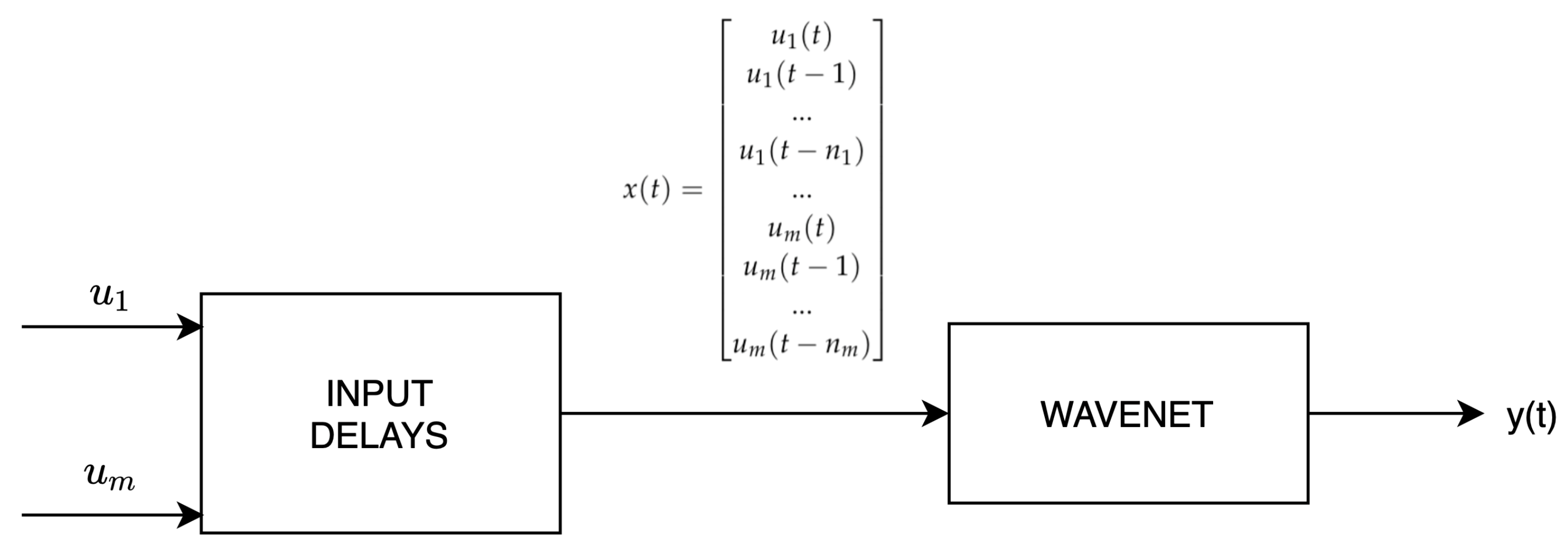
The objective of this work is to evaluate the possibility of implementing a virtual sensor for P M 10 daily mean concentration starting from the data measured by sensors detecting other pollutants and meteorological variables. In particular, the virtual sensors applied in this work are based on N O 2 daily mean concentration and meteorological variables, such as wind speed, rainfall, relative humidity and temperature.
As indicated by the name, virtual sensors can be broadly described as a software that allows us to compute the value of a certain variable without direct measurement considering measurements that are physically/chemically related to the variable that should be reproduced [15]. They assume a key role when it is not possible to place a physical sensor due to any kind of limitations (e.g., unreachable position, high cost). There are two possible approaches to virtual sensor implementation:
1.
Data-driven: in this approach, time series of input and output variables are collected from direct measurement and are used to compute a mathematical, approximated relationship between the measured variables’ and sensors’ output [16];
2.
Deterministic: in this approach, the (eventually approximated) physical/chemical relationships among input and output variables are used to compute the unmeasured variable through the virtual sensor [17].
This work presents a data-driven approach based on wavenet models to implement a P M 10 virtual sensor using N O 2 and meteorological variables. All these variables are strictly related to the phenomena involved in the formation and accumulation of P M 10 in atmosphere; their choice is due to the presence in the literature of low-cost sensors with performances that are adequate [18] enough to identify a virtual sensor, therefore allowing the definition of a low-cost P M 10 measuring network. Wavenets are data-driven models resulting from the integration of wavelet theory and neural network models [19]. Their main applications are related to sound management/filtering [20], even if their nonlinear function approximation (and thus forecasting) properties have been applied with good results also in other fields such as energy systems [19,21]. These approximation properties make them suitable for environmental monitoring and forecasting applications, but still, there is no literature related to their application to reproduce P M 10 or other air quality pollutants. Therefore, since artificial neural networks are widely used in this field [4,22,23], wavenets could also be useful for the definition of a P M 10 virtual sensor. The paper is organized in two main parts, a methodological one (Section 2) where the basics of the artificial neural network, wavelet theory and wavenets are introduced and a second part presenting the evaluation of the results on a test case.

2. Materials and Methods

In this section, the theoretical framework used to derive a virtual air quality sensor based on wavenets [24] is presented.

2.1. Artificial Neural Networks

Artificial Neural Networks (ANNs) are functions approximating human brain behavior, considered as a network of smaller units, called neurons, representing the information processing unit (Figure 1).
Each input x i of the network is multiplied by a corresponding weight w i , analogous to a synaptic force; then all the weighted inputs are added together, including also a bias b term in order to compute the activation level x of the neuron. The output signal y ( x ) is usually a nonlinear function f ( x ) of the activation level. Hence, the typical neuron model is represented as (1):
y ( x ) = f i = 1 d x i × w i + b
where d is the length of the input vector.
The approximation capacity of a single neuron is quite limited; to overcome this, they are collected in layers sharing the same input. The final structure of a neural network is obtained by connecting several layers, as in the case of the two-layer feedforward neural network in Figure 2.
In this case, the output y ( x ) can be computed as:
y ( x ) = g ( L W × f ( I W × x + b 1 ) + b 2 )
where y ( x ) R m 2 is the output of the network, x R d is its input vector, f : R d R m 1 and g : R m 1 R m 2 are the activation functions of the hidden and output layers, respectively, and, finally, m 1 and m 2 are the lengths of the activation function output and the neural network output. The bias terms b 1 , b 2 R m 1 and the weight matrices I W R m 1 × d and L W R m 2 × m 1 are computed during the training phase. Even if the number of layers of an artificial neural network can be higher than 2, following the proof of the Cybenko approximation theorem, and in order to limit the complexity of the network, in real applications only a two layers neural network is used [25].

2.2. Wavelets and Wavenet Models

Wavelets are a family of orthonormal basis functions that can be used to perform transformations among spaces. Their use ranges from function approximation to audio compression [26,27,28]. The wavelet approximation theory is strictly related to multi-resolution analysis [26]. In this context, a function h ( x ) can be approximated using the so-called wavelet (mother) and scaling (father) functions, as:
h ( x ) = k c j 0 ( k ) ϕ j 0 , k ( x ) + j = j 0 k d j ( k ) ψ j , k ( x )
where:
  • c j 0 ( k ) are the scaling coefficients;
  • d j ( k ) are the details (wavelet) coefficient;
  • ϕ j 0 , k ( x ) is the selected scaling (father) function family;
  • ψ j , k ( x ) is the selected wavelet (mother) function family.
The computation of the scaling and wavelet coefficient is strongly connected to the selected wavelet family (considered as the couple wavelet/scaling functions). Up to now, a number of different functions has been considered and are currently used. More details about wavelet transformation can be found in [26,27,28].
Wavenets (wavelet networks) [24] can be considered as a one hidden layer network with wavelets as activation functions. In particular, the wavenet output Y ( x ) for an input x R d can be computed as:
Y ( x ) = W N ( x ) = ( x r ) G + + i = 1 n s a s _ i ϕ ( b s _ i ( ( x r ) Q c s _ i ) + + j = 1 n w a w _ j ψ ( b w _ j ( ( x r ) Q c s _ j )
where ϕ ( z ) = e 0.5 z · z , z = b s _ i ( ( x r ) Q c s _ i is the scaling function, ψ ( t ) = ( m t · t ) e 0.5 t · t , t = b w _ j ( ( x r ) Q c s _ j ) is the wavelet function, x R 1 × d is the row vector input of the wavenet, a s _ i , b s _ i , a w _ i , b w _ i , r R 1 × d , G R d × 1 and Q R d × d are the parameters to be computed during the training.
The comparison between Equations (2) and (4) shows that the wavenet can be considered as a neural network with the function:
f ( · ) = ϕ ( · ) ψ ( · )
as the activation function of the hidden layer.
When the phenomena to model with the wavenet is dynamical, the wavenet is feeded by an input vector x ( t ) that is the output of a time delay phase:
x ( t ) = u 1 ( t ) u 1 ( t 1 ) . . . u 1 ( t n 1 ) . . . u m ( t ) u m ( t 1 ) . . . u m ( t n m )
where u 1 . . . u m are the variables selected to compute the output y ( t ) of the overall system. In this work, since the P M 10 formation, accumulation and removal are clearly dynamical processes, the system structure presented in Figure 3 is used.

3. Results and Discussion

3.1. Case Study and Dataset Definition

The aim of this work is the definition of a virtual sensor to compute P M 10 daily average concentrations starting from the measured data of daily average N O 2 concentration and the measured values of two meteorological variables: average daily wind speed W S , total daily rainfall R F , average daily relative humidity R H and average daily temperature T. The selection of N O 2 as the input variable is due to the fact that its levels are strongly related to P M 10 ones, as they shared some emission drivers (i.e., road traffic, domestic heating) and chemical paths (i.e., formation of secondary inorganic aerosol starting from the ammonium nitrates). On the other hand, the selected meteorological variables can be related to general deposition or dispersion conditions (mainly rainfall and wind speed) or to the formation of secondary aerosol by condensation. Thus, the Y ( x ) in Equation (4) is the daily P M 10 concentration computed by the model, which is referred to as n P M 10 ^ ( x ) from now on. Moreover, the input x of the wavenet function is time dependent, so x = x ( t ) , and it includes both N O 2 concentrations and meteorological variables for the day t and the previous days, as in:
x ( t ) = N O 2 ( t ) N O 2 ( t 1 ) . . . N O 2 ( t n N O 2 ) . . . W S ( t ) W S ( t 1 ) . . . W S ( t n W S ) . . . R F ( t ) R F ( t 1 ) . . . R F ( t n R F ) . . . R H ( t ) R H ( t 1 ) . . . R H ( t n R H ) . . . T ( t ) T ( t 1 ) . . . T ( t n T )
In order to test the presented methodology, a series of models has been trained and validated to reproduce the P M 10 
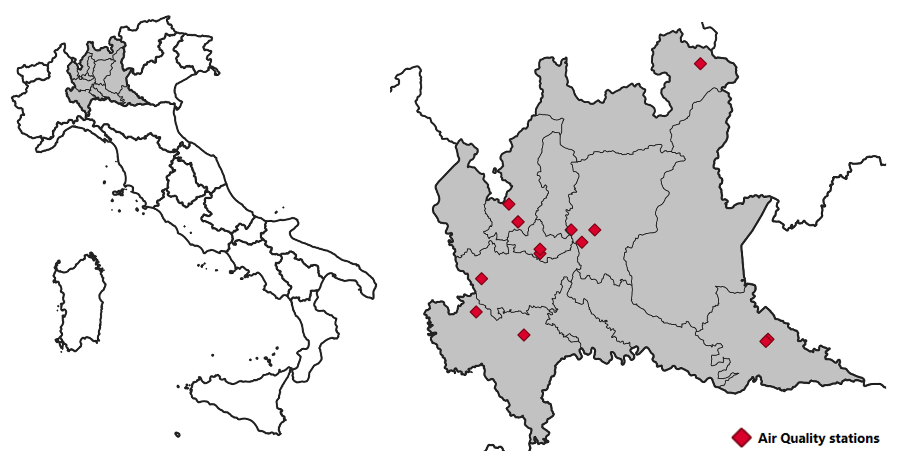
daily mean concentrations starting from different input measured by the Lombardy region monitoring network. The work has been tested using data measured by 14 monitoring stations belonging to the Lombardy region (Italy) monitoring network (Figure 4).
More in detail, the data from year 2019 have been used ( 365 × 14 = 5110 available raw data tuples). The performance evaluation for the different models has been performed using a leave-p-out approach with p = 4 . Following this approach, 100 tests have been performed for each model configuration, with 10 stations being used for the identification, and the data for p = 4 being randomly selected as stations queued in order to define the metastation used for the validation.

3.2. Configuration Tests

In order to evaluate the capability of the methodology presented in Section 2 to compute P M 10 concentrations, all the possible configurations among the input variables have been considered, and the relative models P M 10 = W N ( x ) trained.
In principle, the different configurations can be grouped into three categories:
  • Configurations including only N O 2 concentration as input;
  • Configurations including only meteorological variables as input;
  • Configurations including both N O 2 concentrations and meteorological variables as input.
For each test, an analysis of the memory of the systems, i.e., an evaluation of the performances of varying n N O 2 , n W S , n R F , n R H and n T , has been performed. On the basis of the knowledge of the phenomena related to the formation of P M 10 in atmosphere, a maximum value of 5 days can be considered for these parameters. Each model has been evaluated on the basis of the following three different statistical indexes:
  • Normalized Root Mean Squared Deviation:
    N R M S D = t = 1 T ( P M 10 ( t ) P M 10 ^ ( t ) ) 2 n P M 10 m a x P M 10 m i n
  • Root Mean Squared Error
    R M S E = t = 1 T ( P M 10 ( t ) P M 10 ^ ( t ) ) 2 T
  • Correlation Coefficient
    C o r r e l a t i o n = t = 1 T ( P M 10 ( t ) μ P M 10 ) ( P M 10 ^ ( t ) μ P M 10 ^ ) t = 1 T ( P M 10 ( t ) μ P M 10 ) 2 · t = 1 T ( P M 10 ^ ( t ) μ P M 10 ^ ) 2
where P M 10 ^ ( t ) and P M 10 ( t ) are, respectively, the t-th values of the model output and of the validation dataset, and μ P M 10 ^ and μ P M 10 are their mean values. From the huge set of performed tests, only the best-performing ones are presented in this context, in particular for the combination of multiple input.

3.3. Validation Results

3.3.1. Models with N O 2 as Input

This first class of models includes only N O 2 daily mean concentrations as input. This is due to the fact that P M 10 and N O 2 concentrations are generated by several common emitting activities (i.e., road transport) and that the secondary inorganic fraction of P M 10 is composed, in part, of nitrates, in particular ammonia nitrate, whose formation depends on the N O 2 concentration in atmosphere. Table 1 highlights that the performances are quite good in terms of correlation, with values around 0.74, and acceptable in terms of root mean square error, with a normalised root mean standard deviation (allowing one to compare the root mean square error with respect to the overall variability of the output time series) around 0.1.
From these results, it is clear that an increase in the memory of the system does not lead to significant impacts on the performances and on the behavior of the model. The negligible increase in performances for the test with n N O 2 = 4 does not justify the increasing number of parameters. Table 2 shows the performances for the same configurations for the part of the time series where P M 10 concentrations higher than 30 μ g / m 3 have been measured. The table states that the model has strong difficulties in reproducing high concentrations, as highlighted by the strong decrease in statistical indexes.

3.3.2. Models with Meteorological Variables as Input

The second class of models considers only the meteorological variables as input. These tests allow an assessment of the relative “importance” between meteorology and N O 2 concentration for the computation of P M 10 levels. Table 3 and Table 4 show poor performances, with the limited exception of the cases with temperature T as input. Thus, the performances suggest that the meteorological conditions alone are not enough to estimate P M 10 concentrations, and, so, they may be at best used to increase the performances in addition to the N O 2 concentrations.

3.3.3. Models with N O 2 and Meteorological Variables as Input

The last class of models considers both the meteorological variables and the N O 2 daily mean concentration as input in order to evaluate if the joint use of these information sources leads to an increase in the performances. Table 5 presents the results with N O 2 concentrations coupled to a meteorological variable at a certain time. The performances are in line with that of the models with only N O 2 as an input. Moreover, the combined use of more than one meteorological variable did not lead to a consistent increase in performance (Table 6, Table 7 and Table 8). The only slight improvement can be seen for high concentrations when the temperature is used as input (Table 9, Table 10, Table 11 and Table 12), but also, in this case, the performances seem not to be good enough (correlation coefficient close to 0.52) in the preproduction of the peaks. These results suggest that, to reproduce mean P M 10 levels in this domain, only the N O 2 concentrations should used, thus relying on cheaper sensors. Nevertheless, a bond in the performances exists, which did not allow the reconstruction of peak concentrations.

3.4. Comparison to State-of-the-Art Models

In this section, the comparison of the wavenet approach used in this work with two different state-of-the-art models is presented. The two models are a (1) K-nearest neighbors (KNN) and an (2) artificial neural network-based model, which are often used in this context to capture the dynamic of the P M 10 [29]. The comparison (Table 13) shows how the performances of the best-identified wavenet are strongly better than that of the KNN model and very similar (slightly better for high orders) to that of the ANN ones. Moreover, it has to be stressed how the best model for the wavenet approach ensures these performances with limited complexity and with a limited number of variables (only N O 2 concentration) with respect to the other approaches.
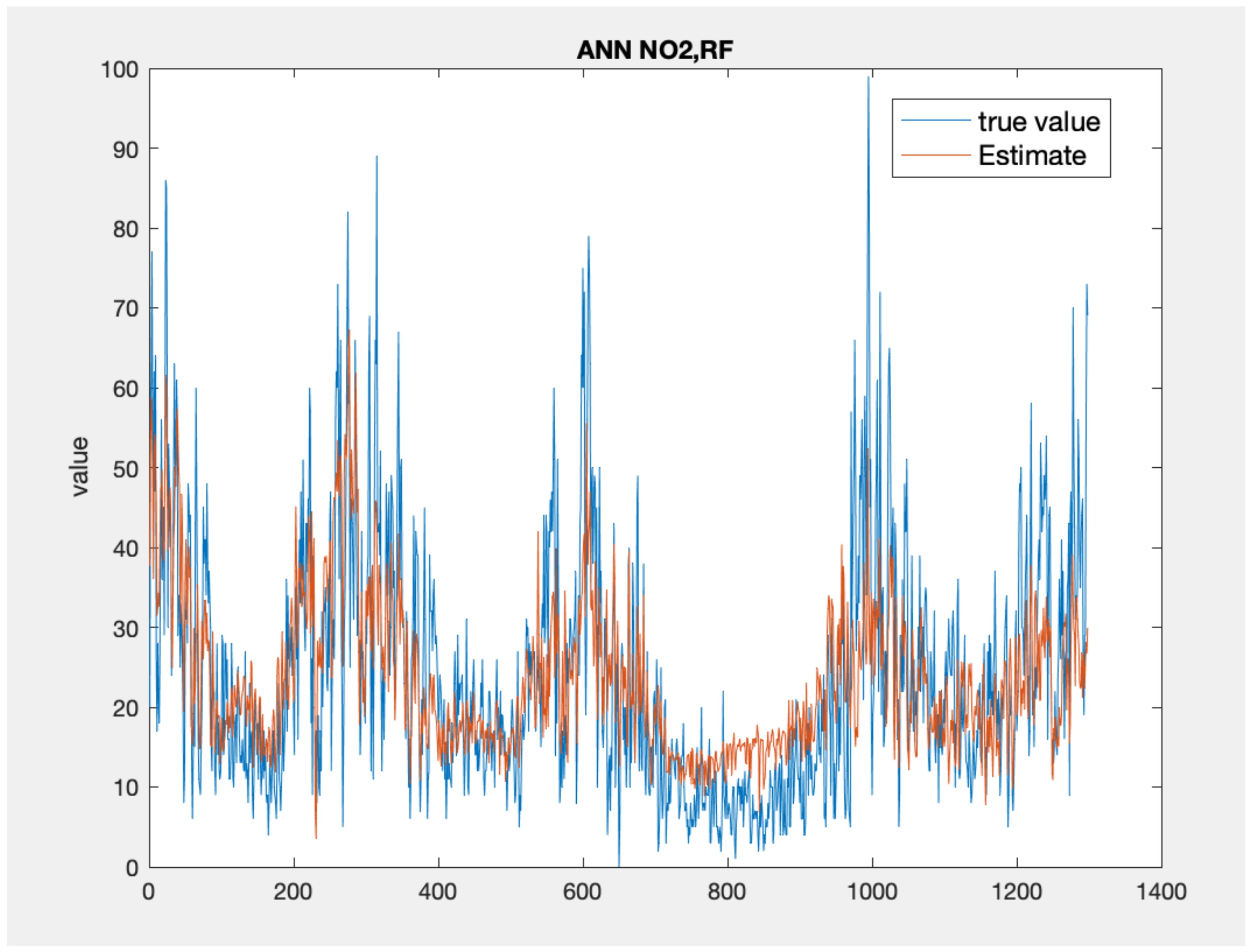
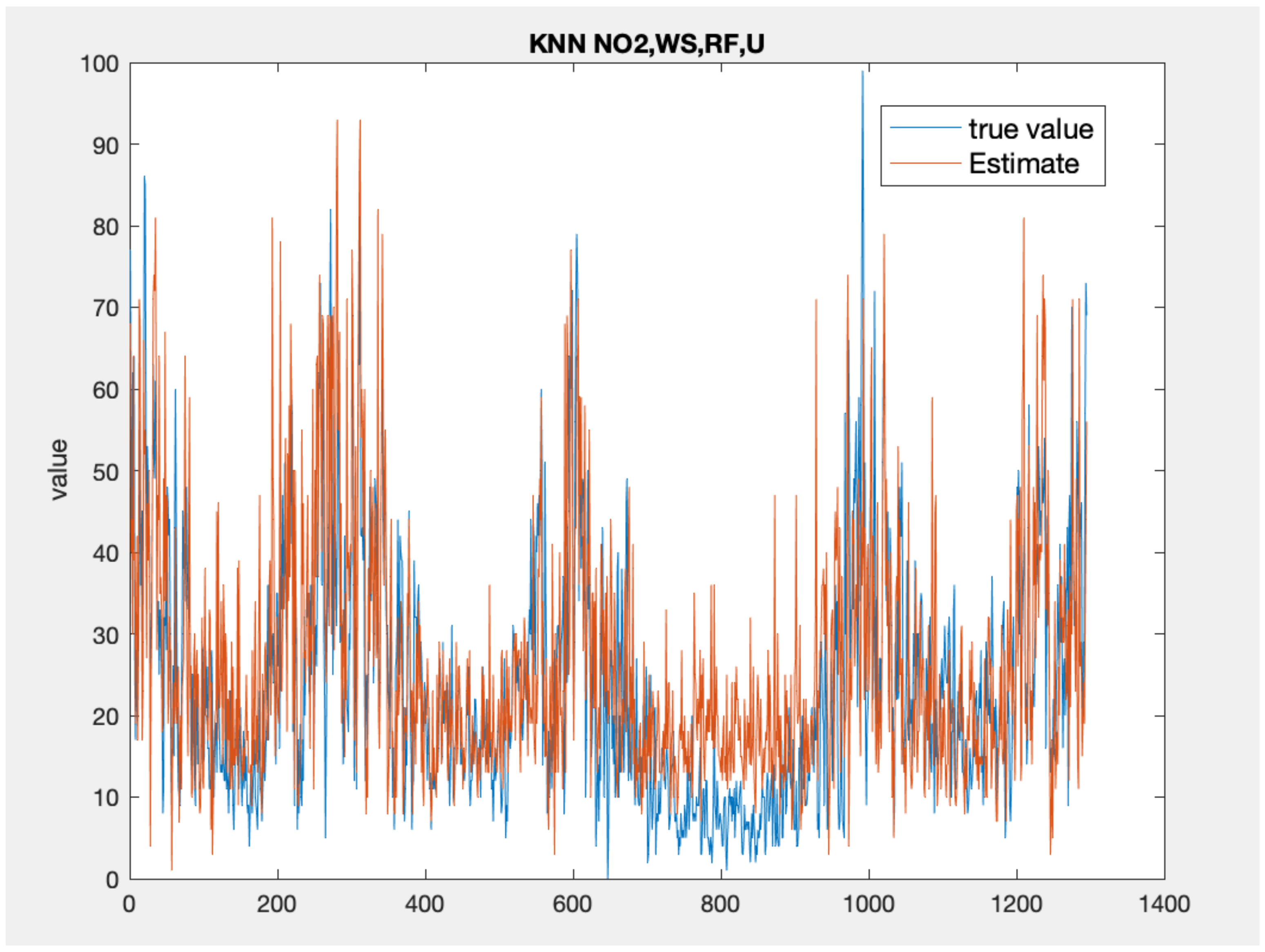
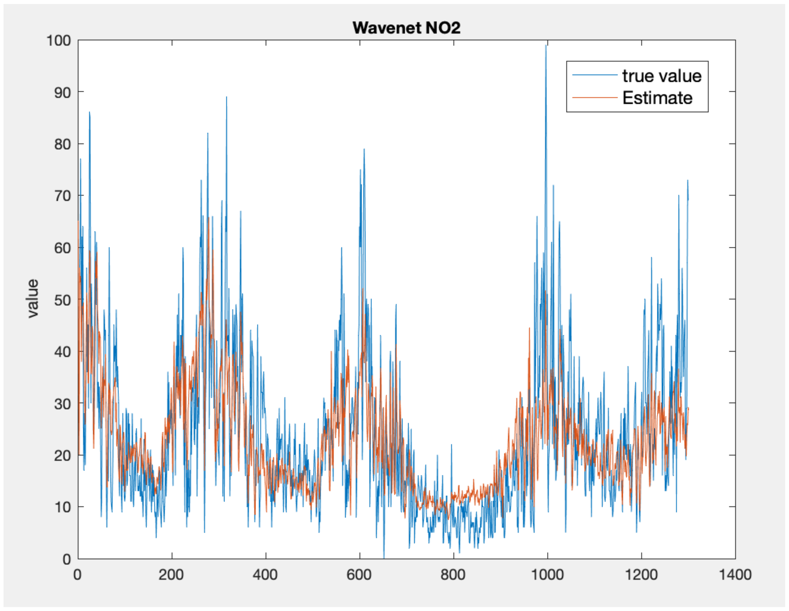
Figure 5, Figure 6 and Figure 7 present the time series plots for the best configuration of wavenet, artificial neural network and KNN models, respectively. As expected, the behaviour of the wavenet and ANN models is very similar, with the first models showing slightly better performances for the low value close to the sample n. 800. In general, the KNN model reproduces higher value but, as also stated by the lower values of correlation coefficient, the time series rarely follows the value and the gradient of the measured values.

4. Conclusions

In this work, a data-driven, wavenet-based virtual sensor for P M 10 daily mean concentration is presented and evaluated. Different model configurations have been tested and evaluated. The methodology has been applied to data measured by the Lombardy regional monitoring network. The results show good agreement between the output of the virtual sensor and the measured data used for validation when the daily mean N O 2 concentration is used as input—in particular, around the mean concentration values. Therefore, the models fail to reproduce the peak concentrations, and this behaviour will not change even if other inputs, such as meteorological data, are used. Nevertheless, the performances show that this approach can be used to produce supporting information to integrate the regional monitoring network that can be made available through app/web services due to a relatively fast computation.

Author Contributions

Conceptualization, C.C., E.T., R.Z.; software, C.C., R.Z.; validation, C.C., E.D.A., M.V.; funding acquisition, M.V. All authors have read and agreed to the published version of the manuscript.

Funding

This research received no external funding.

Conflicts of Interest

The authors declare no conflict of interest.

References

  1. Landrigan, P.; Fuller, R.; Acosta, N.; Adeyi, O.; Arnold, R.; Basu, N.; Baldé, A.; Bertollini, R.; Bose-O’Reilly, S.; Boufford, J.; et al. The Lancet Commission on pollution and health. Lancet 2018, 391, 462–512. [Google Scholar] [CrossRef] [Green Version]
  2. Pope, C., III; Dockery, D.; Spengler, J.; Raizenne, M. Respiratory health and PM10 pollution: A daily time series analysis. Am. Rev. Respir. Dis. 1991, 144, 668–674. [Google Scholar] [CrossRef]
  3. Pope, C., III; Dockery, D. Acute health effects of PM10 pollution on symptomatic and asymptomatic children. Am. Rev. Respir. Dis. 1992, 145, 1123–1128. [Google Scholar] [CrossRef] [PubMed]
  4. Turrini, E.; Carnevale, C.; Finzi, G.; Volta, M. A non-linear optimization programming model for air quality planning including co-benefits for GHG emissions. Sci. Total Environ. 2018, 621, 980–989. [Google Scholar] [CrossRef]
  5. Carnevale, C.; Ferrari, F.; Guariso, G.; Maffeis, G.; Turrini, E.; Volta, M. Assessing the Economic and Environmental Sustainability of a Regional Air Quality Plan. Sustainability 2018, 10, 3568. [Google Scholar] [CrossRef] [Green Version]
  6. Gimez Vilchez, J.; Julea, A.; Peduzzi, E.; Pisoni, E.; Krause, J.; Siskos, P.; Thiel, C. Modelling the impacts of EU countries electric car deployment plans on atmospheric emissions and concentrations. Eur. Transp. Res. Rev. 2019, 11, 40. [Google Scholar] [CrossRef]
  7. Relvas, H.; Miranda, A.; Carnevale, C.; Maffeis, G.; Turrini, E.; Volta, M. Optimal air quality policies and health: A multi-objective nonlinear approach. Environ. Sci. Pollut. Res. 2017, 24, 13687–13699. [Google Scholar] [CrossRef]
  8. Marques, G.; Pires, I.M.; Miranda, N.; Pitarma, R. Air Quality Monitoring Using Assistive Robots for Ambient Assisted Living and Enhanced Living Environments through Internet of Things. Electronics 2019, 8, 1375. [Google Scholar] [CrossRef] [Green Version]
  9. Arroyo, P.; Lozano, J.; Suárez, J. Evolution of Wireless Sensor Network for Air Quality Measurements. Electronics 2018, 7, 342. [Google Scholar] [CrossRef] [Green Version]
  10. Carnevale, C.; Finzi, G.; Pederzoli, A.; Pisoni, E.; Thunis, P.; Turrini, E.; Volta, M. A methodology for the evaluation of re-analyzed PM10 concentration fields: A case study over the PO Valley. Air Qual. Atmos. Health 2015, 8, 533–544. [Google Scholar] [CrossRef]
  11. Candiani, G.; Carnevale, C.; Finzi, G.; Pisoni, E.; Volta, M. A comparison of reanalysis techniques: Applying optimal interpolation and Ensemble Kalman Filtering to improve air quality monitoring at mesoscale. Sci. Total Environ. 2013, 458–460, 7–14. [Google Scholar] [CrossRef]
  12. Carnevale, C.; Finzi, G.; Pederzoli, A.; Turrini, E.; Volta, M.; Ferrari, F.; Gianfreda, R.; Maffeis, G. Impact of pollutant emission reductions on summertime aerosol feedbacks: A case study over the PO valley. Atmos. Environ. 2015, 122, 41–57. [Google Scholar] [CrossRef]
  13. Winkel, A.; Llorens Rubio, J.; Huis in’t Veld, J.W.; Vonk, J.; Ogink, N.W. Equivalence testing of filter-based, beta-attenuation, TEOM, and light-scattering devices for measurement of PM10 concentration in animal houses. J. Aerosol. Sci. 2015, 80, 11–26. [Google Scholar] [CrossRef]
  14. Costa, A.; Guarino, M. Definition of yearly emission factor of dust and greenhouse gases through continuous measurements in swine husbandry. Atmos. Environ. 2009, 43, 1548–1556. [Google Scholar] [CrossRef]
  15. Pathak, D.; Halale, V.P. An Introductory Approach to Virtual Sensors and Its Modelling Techniques. Sci. Eng. Res. 2016, 7, 461–464. [Google Scholar]
  16. Sun, S.; He, Y.; Zhou, S.D.; Yue, Z.J. A Data-Driven Response Virtual Sensor Technique with Partial Vibration Measurements Using Convolutional Neural Network. Sensors 2017, 17, 2888. [Google Scholar] [CrossRef] [Green Version]
  17. Kuo, S.; Zhou, M. Virtual sensing techniques and their applications. In Proceedings of the International Conference on Networking, Sensing and Control, Okayama, Japan, 26–29 March 2009; pp. 31–39. [Google Scholar]
  18. Rai, A.C.; Kumar, P.; Pilla, F.; Skouloudis, A.N.; Sabatino, S.D.; Ratti, C.; Yasar, A.; Rickerby, D. End-user perspective of low-cost sensors for outdoor air pollution monitoring. Sci. Total Environ. 2017, 607–608, 691–705. [Google Scholar] [CrossRef] [Green Version]
  19. Saljooghi, S.; Hezarkarkhani, A. Comparison of WAVENET and ANN for predicting the porosity obtained from well log data. J. Petrol. Sci. Eng. 2014, 123, 172–182. [Google Scholar] [CrossRef]
  20. Van den Oord, A.; Dieleman, S.; Zen, H.; Simonyan, K.; Vinyals, O.; Graves, A.; Kalchbrenner, N.; Senior, A.; Kavukcuoglu, K. WaveNet: A Generative Model for Raw Audio. arXiv 2016, arXiv:1609.03499. [Google Scholar]
  21. Saljooghi, S.; Hezarkarkhani, A. A new approach to improve permeability prediction of petroleum reservois using neural network adaptive wavelet (Wavenet). J. Petrol. Sci. Eng. 2015, 123, 851–861. [Google Scholar] [CrossRef]
  22. Carnevale, C.; Angelis, E.; Finzi, G.; Turrini, E.; Volta, M. Application of data fusion techniques to improve air quality forecast: A case study in the Northern Italy. Atmosphere 2020, 11, 244. [Google Scholar] [CrossRef] [Green Version]
  23. Carnevale, C.; De Angelis, E.; Tagliani, F.; Turrini, E.; Volta, M. A short-term air quality control for PM10 levels. Electronics 2020, 9, 1409. [Google Scholar] [CrossRef]
  24. Sujatha, P. Vibration and Acoustics: Measurement and Signal Analysis; McGraw-Hill Education: Gautam Buddha Nagar, India, 2010. [Google Scholar]
  25. Cybenko, G. Approximation by Superposition of a Sigmoidal Function. Math. Control Signals Syst. 1989, 2, 303–314. [Google Scholar] [CrossRef]
  26. Mallat, S. A Theory for Multiresolution Signal Decomposition The Wavelet Representation. IEEE Trans. Pattern Anal. Mach. Intell. 1989, 11, 674–693. [Google Scholar] [CrossRef] [Green Version]
  27. Zakeri, V.; Naghavi, V.; Safavi, A. Developing real-time wave-net models for non-linear time-varying experimental processes. Comput. Chem. Eng. 2009, 33, 1379–1385. [Google Scholar] [CrossRef]
  28. Postalciouglu, S.; Erkan, K.; Bolat, E.D. Comparison of Wavenet and Neuralnet for System Modeling. In Knowledge-Based Intelligent Information and Engineering Systems; Khosla, R., Howlett, R.J., Jain, L.C., Eds.; Springer: Berlin/Heidelberg, Germany, 2005; pp. 100–107. [Google Scholar]
  29. Carnevale, C.; Finzi, G.; Guariso, G.; Pisoni, E.; Volta, M. Surrogate models to compute optimal air quality planning policies at a regional scale. Environ. Model. Softw. 2012, 34, 44–50. [Google Scholar] [CrossRef]
Figure 1. Typical neuron model.
Electronics 10 02111 g001
Figure 2. Two-layer feedforward neural network structure.
Electronics 10 02111 g002
Figure 3. Wavenet structure.
Electronics 10 02111 g003
Figure 4. Domain and measuring stations.
Electronics 10 02111 g004
Figure 5. Time series comparison between the measured values (blue) and the best wavenet model output ( n N O 2 = 5 , red).
Electronics 10 02111 g005
Figure 6. Time series comparison between the measured values (blue) and the best neural network model output ( n N O 2 , R F = 2 , red).
Electronics 10 02111 g006
Figure 7. Time series comparison between the measured values (blue) and the best KNN model output ( n N O 2 , R F = 5 , red).
Electronics 10 02111 g007
Table 1. N O 2 input configuration performances.
x = { NO 2 }
n N O 2 = 1
c o r r e l a t i o n 0.723
R M S E 10.896
N R M S D 0.1101
n N O 2 = 2
c o r r e l a t i o n 0.722
R M S E 10.927
N R M S D 0.1104
n N O 2 = 3
c o r r e l a t i o n 0.732
R M S E 10.764
N R M S D 0.1087
n N O 2 = 4
c o r r e l a t i o n 0.733
R M S E 10.743
N R M S D 0.1085
n N O 2 = 5
c o r r e l a t i o n 0.742
R M S E 10.575
N R M S D 0.1068
Table 2. N O 2 input configuration performances for P M 10 > 30 μ g / m 3 .
x = { NO 2 }
n N O 2 = 1
c o r r e l a t i o n 0.39
R M S E 11.531
N R M S D 0.1696
n N O 2 = 2
c o r r e l a t i o n 0.39
R M S E 11.481
N R M S D 0.1688
n N O 2 = 3
c o r r e l a t i o n 0.41
R M S E 11.390
N R M S D 0.1675
n N O 2 = 4
c o r r e l a t i o n 0.40
R M S E 11.412
N R M S D 0.1678
n N O 2 = 5
c o r r e l a t i o n 0.40
R M S E 11.444
N R M S D 0.1683
Table 3. Meteorological input configuration performances.
x = { WS } x = { RF } x = { RH } x = { T } x = { RH , T }
n W S = 1 n R F = 1 n R H = 1 n T = 1 n R H , T = 1
c o r r e l a t i o n 0.330.100.1500.4610.47
R M S E 16.73316.62216.38014.80714.736
N R M S D 0.16900.16790.16550.14960.1488
n W S = 2 n R F = 2 n R H = 2 n T = 2 n R H , T = 2
c o r r e l a t i o n 0.370.180.1850.4940.50
R M S E 16.72316.48616.13214.55114.469
N R M S D 0.16890.16650.16300.14700.1462
n W S = 3 n R F = 3 n R H = 3 n T = 3 n R H , T = 3
c o r r e l a t i o n 0.370.230.1710.5030.52
R M S E 16.89916.28316.17614.46714.385
N R M S D 0.17070.16440.16340.14610.1453
n W S = 4 n R F = 4 n R H = 4 n T = 4 n R H , T = 4
c o r r e l a t i o n 0.380.270.1900.5130.513
R M S E 16.91215.901016.08514.34714.474
N R M S D 0.17080.16060.16250.14490.1462
n W S = 5 n R F = 5 n R H = 5 n T = 5 n R H , T = 5
c o r r e l a t i o n 0.3390.300.1830.5140.52
R M S E 16.84615.73016.12614.34814.419
N R M S D 0.17010.15880.16290.14490.1456
Table 4. Meteorological input configuration performances for P M 10 > 30 μ g / m 3 .
x = { WS } x = { RF } x = { RH } x = { T } x = { RH , T }
n W S = 1 n R F = 1 n R H = 1 n T = 1 n U T = 1
c o r r e l a t i o n 0.190.0790.150.350.32
R M S E 12.71112.51712.29611.73211.889
N R M S D 0.18690.18410.18080.17250.1748
n W S = 2 n R F = 2 n R H = 2 n T = 2 n U T = 2
c o r r e l a t i o n 0.1960.1530.180.400.43
R M S E 12.86212.42512.23111.41111.263
N R M S D 0.18910.18270.17990.16780.1656
n W S = 3 n R F = 3 n R H = 3 n T = 3 n U T = 3
c o r r e l a t i o n 0.1850.2120.200.430.40
R M S E 12.93512.27212.19311.22011.536
N R M S D 0.19020.18050.17930.16500.1696
n W S = 4 n R F = 4 n R H = 4 n T = 4 n U T = 4
c o r r e l a t i o n 0.240.2100.170.440.42
R M S E 12.92612.27212.28411.19011.388
N R M S D 0.19010.18050.18060.16460.1675
n W S = 5 n R F = 5 n R H = 5 n T = 5 n U T = 5
c o r r e l a t i o n 0.1920.2200.200.440.45
R M S E 12.97912.24412.17811.16411.193
N R M S D 0.19090.18010.17910.16420.1646
Table 5. N O 2 and one meteorological variable input configuration performance.
x = { NO 2 , WS } x = { NO 2 , RF } x = { NO 2 , RH } x = { NO 2 , T }
n N O 2 , W S = 1 n N O 2 , R F = 1 n N O 2 , R H = 1 n N O 2 , T = 1
c o r r e l a t i o n 0.690.720.710.72
R M S E 11.28510.98710.96910.808
N R M S D 0.11390.11090.11080.1092
n N O 2 , W S = 2 n N O 2 , R F = 2 n N O 2 , R H = 2 n N O 2 , T = 2
c o r r e l a t i o n 0.700.730.720.73
R M S E 11.20710.79610.91610.672
N R M S D 0.11320.10900.11030.1078
n N O 2 , W S = 3 n N O 2 , R F = 3 n N O 2 , R H = 3 n N O 2 , T = 3
c o r r e l a t i o n 0.710.730.720.73
R M S E 11.04210.73510.89010.669
N R M S D 0.11150.10840.11000.1078
n N O 2 , W S = 4 n N O 2 , R F = 4 n N O 2 , R H = 4 n N O 2 , T = 4
c o r r e l a t i o n 0.710.7310.720.74
R M S E 11.00710.67010.90610.543
N R M S D 0.11110.10770.11020.1065
n N O 2 , W S = 5 n N O 2 , R F = 5 n N O 2 , R H = 5 n N O 2 , T = 5
c o r r e l a t i o n 0.7110.7410.710.73
R M S E 10.95010.50010.95410.716
N R M S D 0.11060.10600.11060.1082
Table 6. N O 2 and two meteorological variable input best configuration performances.
x = { NO 2 , x = { NO 2 , x = { NO 2 , x = { NO 2 , x = { NO 2 ,
WS , RF } RH , T } WS , T } RF , RH } RF , T }
n N O 2 , W S , R F = 1 n N O 2 , R H , T = 1 n N O 2 , W S , T = 1 n N O 2 , R F , R H = 1 n N O 2 , R F , T = 1
c o r r e l a t i o n 0.700.720.700.720.73
R M S E 11.13210.85911.10310.87010.768
N R M S D 0.11240.10970.11220.10980.1088
n N O 2 , W S , R F = 2 n N O 2 , R H , T = 2 n N O 2 , W S , T = 2 n N O 2 , R F , R H = 2 n N O 2 , R F , T = 2
c o r r e l a t i o n 0.720.730.690.7250.73
R M S E 10.84410.74311.38510.74810.725
N R M S D 0.10950.10850.11500.10860.1083
n N O 2 , W S , R F = 3 n N O 2 , R H , T = 3 n N O 2 , W S , T = 3 n N O 2 , R F , R H = 3 n N O 2 , R F , T = 3
c o r r e l a t i o n 0.7110.730.720.720.73
R M S E 10.94510.69010.94510.83710.690
N R M S D 0.11050.10800.11060.10950.1080
n N O 2 , W S , R F = 4 n N O 2 , R H , T = 4 n N O 2 , W S , T = 4 n N O 2 , R F , R H = 4 n N O 2 , R F , T = 4
c o r r e l a t i o n 0.720.720.730.710.73
R M S E 10.80310.84910.82310.96510.752
N R M S D 0.10910.10960.10930.11080.1086
n N O 2 , W S , R F = 5 n N O 2 , R H , T = 5 n N O 2 , W S , T = 5 n N O 2 , R F , R H = 5 n N O 2 , R F , T = 5
c o r r e l a t i o n 0.7310.720.720.700.71
R M S E 10.6210.88010.91811.10911.032
N R M S D 0.10720.10990.11030.11220.1114
Table 7. N O 2 and three meteorological variable input configuration performances.
x = { NO 2 , RF , RH , T } x = { NO 2 , WS , RF , RH } x = { NO 2 , WS , RF , T }
n N O 2 , R F , R H , T = 1 n N O 2 , W S , R F , R H = 1 n N O 2 , W S , R F , T = 1
c o r r e l a t i o n 0.720.6920.71
R M S E 10.84111.24110.992
N R M S D 0.10950.11350.1110
n N O 2 , R F , R H , T = 2 n N O 2 , W S , R F , R H = 2 n N O 2 , W S , R F , T = 2
c o r r e l a t i o n 0.720.720.71
R M S E 10.82610.86811.064
N R M S D 0.10940.10980.1118
n N O 2 , R F , R H , T = 3 n N O 2 , W S , R F , R H = 3 n N O 2 , W S , R F , T = 3
c o r r e l a t i o n 0.720.7030.72
R M S E 10.86911.08410.916
N R M S D 0.10970.11190.1098
n N O 2 , R F , R H , T = 4 n N O 2 , W S , R F , R H = 4 n N O 2 , W S , R F , T = 4
c o r r e l a t i o n 0.700.710.721
R M S E 11.09810.03211.163
N R M S D 0.11210.11140.1128
n N O 2 , R F , R H , T = 5 n N O 2 , W S , R F , R H = 5 n N O 2 , W S , R F , T = 5
c o r r e l a t i o n 0.690.700.714
R M S E 11.32411.20711.071
N R M S D 0.11440.11320.1118
Table 8. N O 2 and four meteorological variable input configuration performances.
x = { NO 2 , WS , RF , RH , T }
n N O 2 , W S , R F , R H , T = 1
c o r r e l a t i o n 0.70
R M S E 11.046
N R M S D 0.1116
n N O 2 , W S , R F , U , T = 2
c o r r e l a t i o n 0.72
R M S E 10.926
N R M S D 0.1104
n N O 2 , W S , R F , U , T = 3
c o r r e l a t i o n 0.73
R M S E 10.788
N R M S D 0.1090
n N O 2 , W S , R F , U , T = 4
c o r r e l a t i o n 0.71
R M S E 11.632
N R M S D 0.1127
n N O 2 , W S , R F , U , T = 5
c o r r e l a t i o n 0.71
R M S E 11.297
N R M S D 0.1141
Table 9. N O 2 one meteorological variable input configuration performance for P M 10 > 30 μ g / m 3 .
x = { NO 2 , WS } x = { NO 2 , RF } x = { NO 2 , RH } x = { NO 2 , T }
n N O 2 , W S = 1 n N O 2 , R F = 1 n N O 2 , R H = 1 n N O 2 , T = 1
c o r r e l a t i o n 0.3810.390.3920.39
R M S E 12.17611.49211.47411.445
N R M S D 0.17910.16900.16870.1683
n N O 2 , W S = 2 n N O 2 , R F = 2 n N O 2 , R H = 2 n N O 2 , T = 2
c o r r e l a t i o n 0.390.4010.4220.49
R M S E 11.97011.45611.28010.817
N R M S D 0.17600.16850.16590.1591
n N O 2 , W S = 3 n N O 2 , R F = 3 n N O 2 , R H = 3 n N O 2 , T = 3
c o r r e l a t i o n 0.3820.4130.4060.50
R M S E 12.08611.38411.46710.744
N R M S D 0.17770.16740.16860.1580
n N O 2 , W S = 4 n N O 2 , R F = 4 n N O 2 , R H = 4 n N O 2 , T = 4
c o r r e l a t i o n 0.400.4050.3950.51
R M S E 11.93811.43811.55310.671
N R M S D 0.17560.16820.16990.1569
n N O 2 , W S = 5 n N O 2 , R F = 5 n N O 2 , R H = 5 n N O 2 , T = 5
c o r r e l a t i o n 0.400.4250.4020.52
R M S E 11.85511.31111.49810.570
N R M S D 0.17430.16630.16910.1554
Table 10. N O 2 and two meteorological variable input best configuration performances for P M 10 > 30 μ g / m 3 .
x = { NO 2 , x = { NO 2 , x = { NO 2 , x = { NO 2 , x = { NO 2 ,
WS , RF } RH , T } WS , T } RF , RH } RF , T }
n N O 2 , W S , R F = 1 n N O 2 , U , T = 1 n N O 2 , W S , T = 1 n N O 2 , R F , U = 1 n N O 2 , R F , T = 1
c o r r e l a t i o n 0.3940.420.450.3940.44
R M S E 12.05811.24611.44511.45811.160
N R M S D 0.17730.16540.16830.16850.1641
n N O 2 , W S = 2 n N O 2 , U , T = 2 n N O 2 , W S , T = 2 n N O 2 , R F , U = 2 n N O 2 , R F , T = 2
c o r r e l a t i o n 0.390.5030.470.4140.485
R M S E 11.97010.75011.36711.36410.832
N R M S D 0.17600.15810.16720.16710.1593
n N O 2 , W S = 3 n N O 2 , U , T = 3 n N O 2 , W S , T = 3 n N O 2 , R F , U = 3 n N O 2 , R F , T = 3
c o r r e l a t i o n 0.3820.490.470.400.49
R M S E 12.08610.89511.23711.57510.825
N R M S D 0.17770.16020.16520.17020.1592
n N O 2 , W S = 4 n N O 2 , U , T = 4 n N O 2 , W S , T = 4 n N O 2 , R F , U = 4 n N O 2 , R F , T = 4
c o r r e l a t i o n 0.400.500.510.400.51
R M S E 11.93810.91910.83911.65810.667
N R M S D 0.17560.16060.15940.17140.1569
n N O 2 , W S = 5 n N O 2 , U , T = 5 n N O 2 , W S , T = 5 n N O 2 , R F , U = 5 n N O 2 , R F , T = 5
c o r r e l a t i o n 0.400.5140.520.400.49
R M S E 11.85510.70710.70311.63210.856
N R M S D 0.17430.15750.15740.17110.1597
Table 11. N O 2 and three meteorological variable input configuration performances for P M 10 > 30 μ g / m 3 .
x = { NO 2 , RF , RH , T } x = { NO 2 , WS , RF , RH } x = { NO 2 , WS , RF , T }
n N O 2 , R F , R H , T = 1 n N O 2 , W S , R F , R H = 1 n N O 2 , W S , R F , T = 1
c o r r e l a t i o n 0.4300.3900.436
R M S E 11.20111.66011.444
N R M S D 0.16470.17150.1683
n N O 2 , R F , R H , T = 2 n N O 2 , W S , R F , R H = 2 n N O 2 , W S , R F , T = 2
c o r r e l a t i o n 0.5030.4070.462
R M S E 10.72011.86311.275
N R M S D 0.15760.17440.1658
n N O 2 , R F , R H , T = 3 n N O 2 , W S , R F , R H = 3 n N O 2 , W S , R F , T = 3
c o r r e l a t i o n 0.490.3810.478
R M S E 10.94512.10311.063
N R M S D 0.16100.17800.1627
n N O 2 , R F , R H , T = 4 n N O 2 , W S , R F , R H = 4 n N O 2 , W S , R F , T = 4
c o r r e l a t i o n 0.5030.3960.498
R M S E 10.89212.07710.846
N R M S D 0.16020.17760.1595
n N O 2 , R F , R H , T = 5 n N O 2 , W S , R F , R H = 5 n N O 2 , W S , R F , T = 5
c o r r e l a t i o n 0.5110.3990.518
R M S E 10.75611.95310.678
N R M S D 0.15820.17580.1570
Table 12. N O 2 and four meteorological variable input configuration performances for P M 10 > 30 μ g / m 3 .
x = { NO 2 , WS , RF , RH , T }
n N O 2 , W S , R F , R H , T = 1
c o r r e l a t i o n 0.425
R M S E 11.484
N R M S D 0.1689
n N O 2 , W S , R F , R H , T = 2
c o r r e l a t i o n 0.494
R M S E 11.067
N R M S D 0.1627
n N O 2 , W S , R F , R H , T = 3
c o r r e l a t i o n 0.484
R M S E 11.191
N R M S D 0.1646
n N O 2 , W S , R F , R H , T = 4
c o r r e l a t i o n 0.492
R M S E 11.107
N R M S D 0.1633
n N O 2 , W S , R F , R H , T = 5
c o r r e l a t i o n 0.522
R M S E 10.875
N R M S D 0.1599
Table 13. Best configuration performances.
WT ( x = { NO 2 } )ANN ( x = { NO 2 , RF } )KNN ( x = { NO 2 , WS , RF , U } )
n N O 2 = 1 n N O 2 , R F = 1 n N O 2 , W S , R F , U = 1
c o r r e l a t i o n 0.7230.720.523
R M S E 10.89610.94014.860
N R M S D 0.11010.11050.1501
n N O 2 = 2 n N O 2 , R F = 2 n N O 2 , W S , R F , U = 2
c o r r e l a t i o n 0.7220.7320.581
R M S E 10.92710.65114.082
N R M S D 0.11040.10760.1422
n N O 2 = 3 n N O 2 , R F = 3 n N O 2 , W S , R F , U = 3
c o r r e l a t i o n 0.7320.720.59
R M S E 10.76410.87713.904
N R M S D 0.10870.10990.1404
n N O 2 = 4 n N O 2 , R F = 4 n N O 2 , W S , R F , U = 4
c o r r e l a t i o n 0.7330.7130.61
R M S E 10.74310.90913.628
N R M S D 0.10850.11020.1377
n N O 2 = 5 n N O 2 , R F = 5 n N O 2 , W S , R F , U = 5
c o r r e l a t i o n 0.7420.730.634
R M S E 10.57510.67513.435
N R M S D 0.10680.10780.1357
Publisher’s Note: MDPI stays neutral with regard to jurisdictional claims in published maps and institutional affiliations.

