Benchmarking GHG Emissions Forecasting Models for Global Climate Policy

Abstract

Climate change and pollution fighting have become prominent global concerns in the twenty-first century. In this context, accurate estimates for polluting emissions and their evolution are critical for robust policy-making processes and ultimately for solving stringent global climate challenges. As such, the primary objective of this study is to produce more accurate forecasts of greenhouse gas (GHG) emissions. This in turn contributes to the timely evaluation of the progress achieved towards meeting global climate goals set by international agendas and also acts as an early-warning system. We forecast the evolution of GHG emissions in 12 top polluting economies by using data for the 1970–2018 period and employing six econometric and machine-learning models (the exponential smoothing state-space model (ETS), the Holt–Winters model (HW), the TBATS model, the ARIMA model, the structural time series model (STS), and the neural network autoregression model (NNAR)), along with a naive model. A battery of robustness checks is performed. Results confirm a priori expectations and consistently indicate that the neural network autoregression model (NNAR) presents the best out-of-sample forecasting performance for GHG emissions at different forecasting horizons by reporting the lowest average RMSE (root mean square error) and MASE (mean absolute scaled error) within the array of predictive models. Predictions made by the NNAR model for the year 2030 indicate that total GHG emissions are projected to increase by 3.67% on average among the world’s 12 most polluting countries until 2030. Only four top polluters will record decreases in total GHG emissions values in the coming decades (i.e., Canada, the Russian Federation, the US, and China), although their emission levels will remain in the upper decile. Emission increases in a handful of developing economies will see significant growth rates (a 22.75% increase in GHG total emissions in Brazil, a 15.75% increase in Indonesia, and 7.45% in India) that are expected to offset the modest decreases in GHG emissions projected for the four countries. Our findings, therefore, suggest that the world’s top polluters cannot meet assumed pollution reduction targets in the form of NDCs under the Paris agreement. Results thus highlight the necessity for more impactful policies and measures to bring the set targets within reach.

1. Introduction

Along with climate change, air pollution is one of the most serious environmental hazards to human health, estimated to cause 7 million premature deaths per year [1]. The economic consequences of air pollution are dire, as estimates indicate $5 trillion in welfare losses and 225 billion in lost income [2,3].

Air pollution includes greenhouse gas (GHG) emissions that warm the earth’s surface and atmosphere [4]. GHG refer to the sum of seven gases that have direct effects on climate change: carbon dioxide (CO₂), methane (CH4), nitrous oxide (N2O), chlorofluorocarbons (CFCs), hydrofluorocarbons (HFCs), perfluorocarbons (PFCs), sulfur hexafluoride (SF6), and nitrogen trifluoride (NF3) [5].

Understanding the urgency of more vigorous climate combat, decisive steps have been taken at the global level. The United Nations Framework Convention on Climate Change (UNFCCC) adopted the Kyoto Protocol (1997) and the Paris Agreement (2015) [6]. The Paris Agreement, signed in December 2015, gathered all signatory countries under a common goal toward making significant efforts to tackle climate change and air pollution [7,8]. The Paris Agreement is meant to improve upon and replace the Kyoto Protocol, an earlier international treaty designed to curb the release of GHG, whose effectiveness has been heavily criticized because the world’s two top carbon dioxide-emitting countries, China and the United States, chose not to be part of the agreement [9]. In contrast, the 2015 Paris agreement has been signed by nearly every country in the world (together responsible for more than 90 percent of global emissions), with 190 of the signatory countries (including the US and China) going further and having underlined their support with formal approval. As such, while before the Paris Conference the signatory countries submitted carbon reduction targets (i.e., “intended nationally determined contributions” or INDCs), these targets subsequently became “nationally determined contributions” or NDCs after the formal approval of the agreement [10]. Hence, the Paris Agreement and the attainment of long-term climate targets are built around these NDCs representing each country’s efforts to cut national emissions and adapt to climate change consequences. Given the heterogeneity in circumstances, resources, and capabilities, the agreement was developed so that each country establishes their own commitments in terms of how much they can contribute to the 2030 Agenda. However, almost all submitted NDCs contain a target to reduce polluting emissions by a specific percentage over a specified period, in most cases, the first established deadline being 2030. However, while signatory parties are legally required to establish an NDC under the Paris agreement and to take actions to accomplish it, the NDC itself is not legally binding or enforceable pledge [11].

Considering the GHG emission mitigation targets that most world countries have set for 2030 and/or 2050 under the Paris agreement, the total GHG emissions were expected to decline significantly in the aftermath of its adoption and to continue a decreasing trend over the next decades. However, the vast majority of world economies are yet to deliver on their pledges [12].

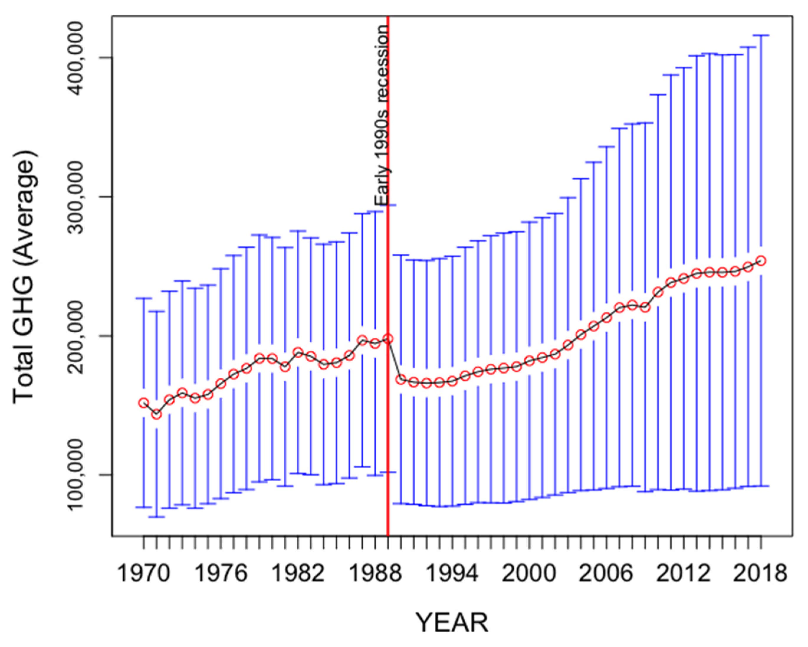
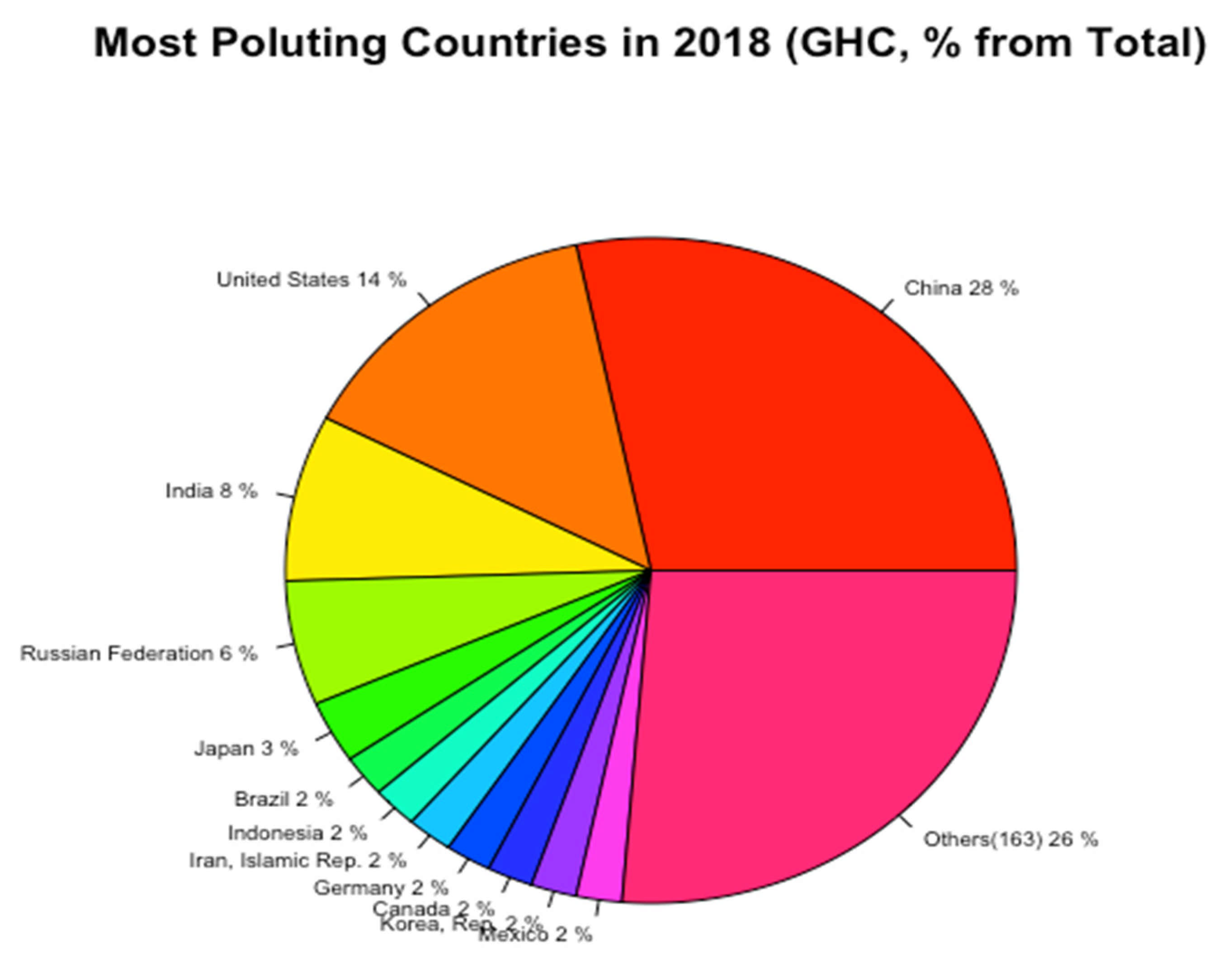
Data employed in our study backs this finding. Figure 1 shows that on average total GHG emissions have continued to increase after 2015, although there is high heterogeneity across countries at the world level when it comes to their contribution to world pollution. Figure 2 highlights that only a handful of countries significantly contributed to world pollution over the 1970–2018 period. Specifically, the main culprits reflected in Figure 2 are the US, with a mean annual value for total GHG emissions measured in kt of CO₂ equal to 6,134,747 over the 49-year period, closely followed by China with 5,439,570 kt average annual GHG over the same period and at some distance by the Russian Federation, which registered 2,635,846 kt average annual GHG emissions. The rhythm of emissions growth has also been heterogenic at the world level over the past decades, as our study will further reflect. Overall, global greenhouse gas emissions have risen considerably since 1970, showing a 67.31% increase by 2018 (when total GHG emissions in kt of CO₂ equivalent at world level registered a mean value of 254,047.3) relative to their 1970 levels (mean value of 151,837.9 kt of CO₂ equivalent). This translates into an increase of 102,209.4 kt CO₂ in absolute terms over the 1970–2018. Over the entire 49-year period, interim short-term reversals followed economic contractions, with a sharper decrease during the 1990s economic recession caused by the Gulf War and subsequent oil price shocks.

This incongruence between policy targets and the current reality is particularly worrying given that top polluters continue to show significant increases in total GHG emissions and highlights the necessity of more impactful policies and measures to bring the set targets within reach. Consequently, accurate and robust forecasts for polluting emissions are needed for an effective and efficient policy-making process. The issue is timely, as countries must juggle post-pandemic recovery and bend the emission trends [13]. However, the task is particularly challenging, as the world should halve annual greenhouse gas emissions in the next eight years to keep global warming below 1.5 °C this century, and thus meet the aspirational goal of the Paris Agreement [14]. Other studies report the need for a cut of total GHG emissions by 7.6 percent each year between 2020 and 2030 to stay on track toward the 1.5 °C temperature goal of the Paris Agreement [15]. Current statistics show a rapid recovery of economic activity and increasing emissions as energy demand soars [16].

Unsurprisingly, polluting emissions have steadily drawn the attention of academics and policymakers over the past decades, and national and international agencies increasingly employ forecasts of polluting emissions in their policy-making process. Consequently, producing accurate estimates for GHG emissions and their evolution is critical for robust policy-making processes and ultimately for solving global climate challenges [17]. This in turn is an important motivator for this study, which intends to identify the over-performing predictive model in terms of forecasting accuracy for total GHG emissions and subsequently apply it for producing forecasts for GHG emissions in top-emitting countries over long forecasting horizons, covering the first benchmark set for individual pledges within the Paris agreement, i.e., 2030.

Unlike most studies in the existing literature that investigate driving factors for polluting emissions, we take a univariate approach. This further brings two important advantages. First, it eliminates the challenge of identifying the right mix of macroeconomic, social, and financial variables that are potential impact factors for polluting emissions, and thus eliminates the risk of model misspecification, with further gains in terms of increasing estimation efficiency. Second, and most importantly, our approach allows us to produce forecasts for a validated leading indicator, independent of other variables.

Considering the above considerations, this study makes several contributions to the extant literature, as follows.

First, we employ a wider variety of candidate predictive models, including econometric and machine-learning methods, and perform a battery of robustness checks to assure that the best-performing out-of-sample forecasting model is identified. As we are more concerned with prediction accuracy than in-sample information, and in light of the previous literature, we a-priori expect machine learning methods to over-perform.

Secondly, we use a more relevant metric for air pollution, GHG emissions, instead of CO₂ emissions that are usually employed in previous studies. Consequently, by including a more accurate indicator of air pollution (i.e., CO₂ emissions account for approximately 76 percent of total GHG emissions, according to the Center for Climate and Energy Solutions [18], estimation results are more relevant for policymakers. To this end, this study uses data for the 1970–2018 period provided by the World Development Indicators (WDI) database of the World Bank.

Thirdly, unlike most of the aforementioned previous studies that focus only on a single country or cover at most a handful of economies, this study includes the 12 most polluting countries in the world, which are responsible together for around 75% of total GHG emissions at world level. This contributes to assuring the robustness of the forecasting method and further increases the relevance of results for policymakers.

Results of this study confirm prior expectations and find that overall on average, the neural network autoregression model (NNAR) presents the best out-of-sample forecasting performance for GHG emissions over a long forecasting horizon by reporting the lowest average RMSE within the array of predictive models. Results further show that the world’s top polluters will not meet assumed GHG emissions’ reduction targets under the Paris agreement, and thus more impactful policies and measures are needed to bring the set goals within reach.

The remainder of the paper is organized as follows. The next section gives an overview of the related literature. Next, Section 3 explains the data and methodology employed in the empirical investigation, while Section 4 presents and discusses the estimation results and the performed robustness checks. Finally, Section 5 concludes the study.

2. Literature Review

The environmental Kuznets curve (EKC) theory [19,20] states that pollution rises with the economic expansion until a certain level of wealth is achieved, at which point emissions begin to decline, implying an inverted U-shaped link between environmental degradation and income [21]. Overall, mixed results were obtained from previous research that looked at the presence of the EKC in different countries and across different time periods [22]. As a result, the topic of how economic growth and environmental quality are related (i.e., the form of the environmental Kuznets curve) continues to be contentious [23]. As such, on one hand, the EKG hypothesis has been validated empirically by numerous studies (among others, [6,24,25,26]). However, on the other hand, a bidirectional causality has also been repeatedly encountered [27], thus suggesting that emissions can also be a leading indicator of growth.

Moreover, besides its proven impact on economic growth, air pollution has a substantial influence on public health [28]. Hence, previous studies confirmed that polluting emissions are also a leading indicator for various health variables [29] and for mortality [30,31]. These effects have been found in both long-term studies, which have followed cohorts of exposed individuals over time, and in studies that connect day-to-day fluctuations in air pollution and health [32]. Moreover, there is mounting evidence that indoor air pollution is a severe concern to human health in addition to ambient air quality, particularly in low-income nations where biomass fuels are still used as an energy source [33]. All these findings further highlight the importance of combating climate change.

As such, given its validated role as an impact factor for important socio-economic variables, the primary objective of this study is to produce more accurate forecasts of GHG emissions. This in turn contributes to the timely evaluation of the progress achieved toward meeting global climate goals set by international agendas and also acts as an early-warning system when projections show that the state of affairs does not reflect policy statements and formal pledges are not followed by concrete measures and results. Hence, results of this study are also important for policymakers to incorporate forecasts of polluting emissions in their policy-making process.

However, time series analysis and forecasting remain challenging tasks [34], and air pollution prediction is no exception [35]. Broadly, based on the work of [36] prediction models pertain to two main cultures or schools of thought [37], each with its benefits and drawbacks [38]: (i) econometrics, or statistical methods, a category that covers many familiar models [39], and (ii) machine learning (self-learning systems, capable of learning from data to improve their performance). Their two common goals, information, and predictability [40] are differently prioritized, with statistical methods focusing on inference, whereas machine-learning techniques concentrate on prediction [41]. As the British statistician George Box has famously put it: “All models are wrong, but some are useful.” Consequently, the aim in time-series forecasting should be to identify the best predictive model within a pool of candidates and employ it to produce forecasts for the series of interest. This study does not deviate from this goal. Previous studies that attempt to model and forecast univariate polluting emission time series (most often CO₂) primarily employ statistical methods, including the logistic equation [42], the ARIMA [43], and the ARIMA, Holt–Winters, exponential smoothing, and singular spectrum analysis (SSA) [44]. In the second category, we encounter among others [45] that use extreme learning machines based on particle swarm optimization to predict CO₂ emissions in Hebei, ref. [46] that use an artificial neural network (ANN) to predict carbon emission intensity for Australia, Brazil, China, India, and the USA, and [47], which employ a neural network model for forecasting the CO₂ emission produced by the cereal sector in a southern Italy region. 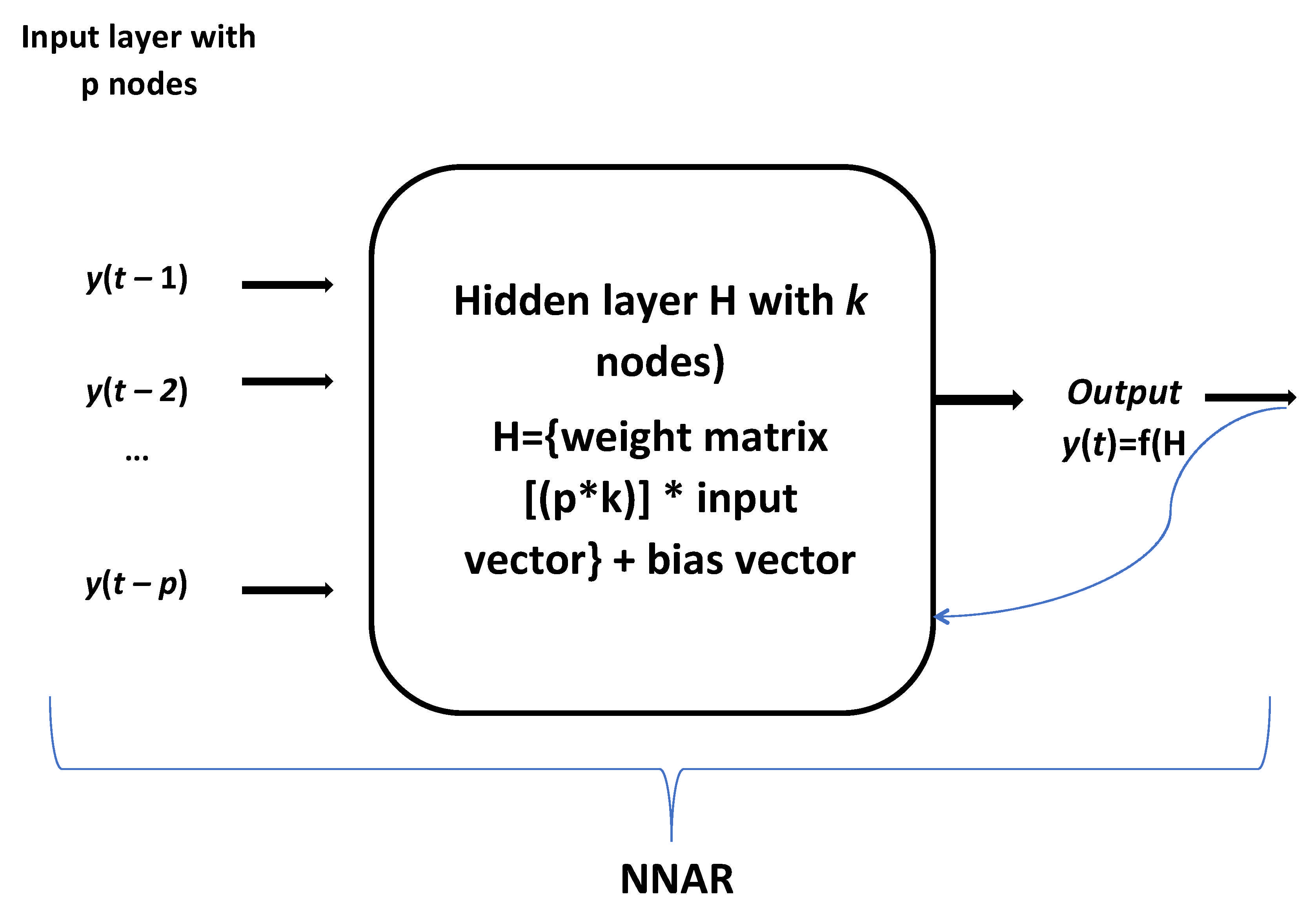Overall, previous studies confirm that nonlinear models can capture the nonlinear pattern of real-world data, and thus overcome the limitation of linear models, improving their prediction performance [48]. Additionally, artificial neural networks (ANN) are found to be useful in time series modeling where past values of a variable of interest are used to determine its future values [49].

In this study, we attempt to forecast the evolution of GHG emissions by employing six candidate models belonging to both the aforementioned categories. As such, we estimate the innovations state-space models for exponential smoothing (ETS), the Holt–Winters (HW) model, the autoregressive integrated moving average (ARIMA) model, the trigonometric ETS state-space model with Box-Cox transformation, ARMA errors, trend and seasonal components (TBATS) model, the structural time series model (STS) and the neural network autoregression (NNAR) model. Additionally, a naive model is also employed for comparative purposes.

Similar approaches in the literature, but with application on other time series, include the study by [50], which estimate and report the forecasting performance of nine models for the price of gold, concluding that on average, the exponential smoothing model is providing the best forecasts in terms of the lowest root mean squared error. Similarly, ref. [51] uses seven automated forecasting techniques, including statistical and machine learning models, for explaining and predicting the evolution of CO₂ emissions in Bahrain and identify the NNAR model to provide the most accurate out-of-sample forecasts. More recently, ref. [34] also predicted the evolution of Bahrain’s CO₂ emissions by employing a neural network time series nonlinear autoregressive model, the Gaussian process regression model, and Holt’s method, to agree that the NNAR model is outperforming the other candidates. Ref. [52] also employs four of the techniques applied in this investigation (i.e., ARIMA, ETS, NNAR, and TBATS) along with their feasible hybrid combinations to forecast the second wave of COVID-19 hospitalizations in Italy, concluding that the best single models were NNAR and ARIMA, and that the best hybrid models always included a NNAR process. Finally, ref. [53] employ statistical and deep learning methods to forecast long-term pollution trends for the two categories of particulate matter (PM) in a major city in eastern India, i.e., Kolkata. They conclude that statistical methods (i.e., auto-regressive (AR), seasonal auto-regressive integrated moving average (SARIMA) and Holt–Winters) outperform deep learning methods for their data. However, they argue that the results might be due to the limited data available, and that with a higher quantity of data and higher frequency and forecasting horizon, deep-learning models would out-perform.

All of these works bring important results for the global climate fight related literature. However, most of these works have a narrow interest (i.e., most are single-country studies, as seen above) and most importantly, they do not strongly defend their results robustness. The vast majority stops at evaluating the predictive ability of alternative models by reporting various forecasting accuracy metrics. [34] employs the root mean square errors (RMSE) to this end, whereas [53] estimate both RMSE and MAE, and [52] reports MAE, MAPE, MASE, and RMSE metrics. Nonetheless, except [51] that reports the KSPA test, other studies do not estimate and present statistical tests for multiple forecast comparisons and thus, do not investigate the hypothesis whether forecasts are significantly different, defending their results. Additionally, none of these previous works have re-estimated the models by employing an alternative forecasting technique (i.e., recursive window, changing window length, various time series slitting rules, etc.).

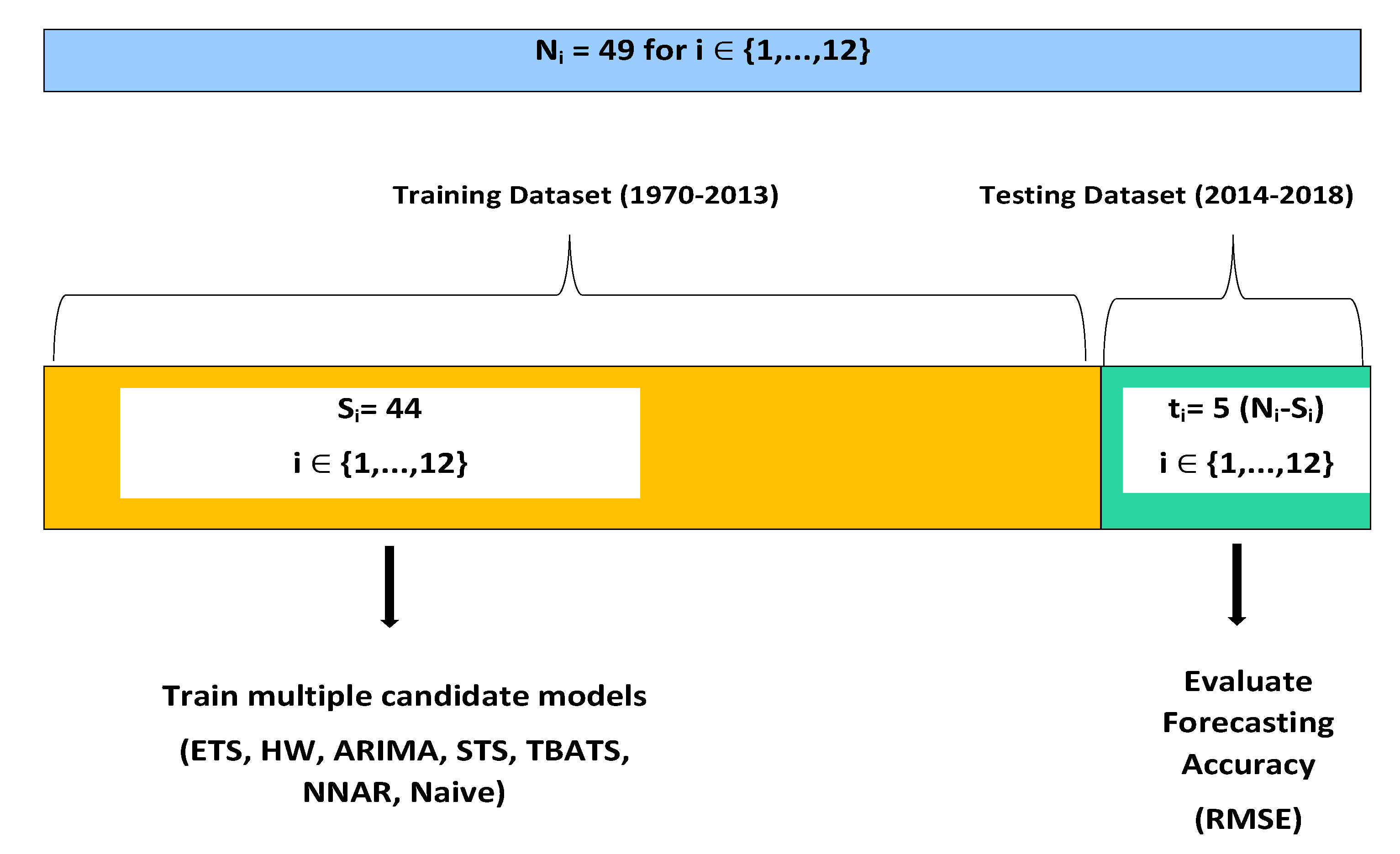
In this study, results’ robustness is assured firstly by employing out-of-sample forecasting on a holdout sample of observations and investigating the accuracy of several forecasting methods in comparative perspective, then by reassessing the predictive ability of candidate models via the recursive window forecasting technique, and finally by performing all estimations for 12 different top polluting countries, responsible for around ¾ of total GHG emissions at world level. Moreover, applying the Kolmogorov–Smirnov (KS) predictive accuracy test (KSPA) proposed by [54] and the Diebold–Mariano (DM) test introduced by [55] and developed by [56] further contributes to testing the over-performance of the best predictive model and assures our results’ robustness.

Additionally, a further advantage of our approach consists in the fact that the employment of standard econometric methods together with machine-learning techniques in estimations and predictions allows comparison with previous results from the literature.

3. Materials and Methods

3.1. Data

3.1.1. Database

This study uses annual data on total GHG emissions measured in kt of CO₂ for the period 31 December 1970–31 December 2018, thus covering a total of 49 years. The source of data is the World Development Indicators (WDI) database of the World Bank (Data source: https://data.worldbank.org/indicator/EN.ATM.GHGT.KT.CE, accessed on 8 November 2021).

In the first stage, GHG data were extracted from the WDI for all countries included in the database, thus resulting in a sample of 205 individual economies. Then, we have removed countries for which data were unavailable over the entire period, resulting in the final sample of 175 countries and 8575 annual observations included in the analysis.

An exploratory analysis aimed at uncovering the state of affairs was subsequently performed.

3.1.2. GHG Emissions by Country, Top Polluters and Historical Trends

Table 1. Greenhouse Gas Emissions by Top Emitters, 2018 and emission trends (1970–2018).

Country	GHG Emissions 2018 (Total, kt of CO2)	Region	Income Category	% Change (Relative to 2015)	% Change (Relative to 1970)
China	12,355,240	East Asia & Pacific	Upper middle	4.18	559.31
United States	6,023,620	North America	High income	0.33	11.54
India	3,374,990	South Asia	Lower middle	10.16	352.11
Russian Federation	2,543,400	Europe & Central Asia	Upper middle	2.73	13.50
Japan	1,186,770	East Asia & Pacific	High income	−6.19	26.10
Brazil	1,032,640	Latin America & Caribbean	Upper middle	−4.62	−18.11
Indonesia	969,580	East Asia & Pacific	Lower middle	13.80	185.44
Iran, Islamic Rep.	828,280	Middle East & North Africa	Upper middle	5.31	484.04
Germany	806,090	Europe & Central Asia	High income	−4.88	−37.35
Canada	724,930	North America	High income	2.40	46.46
Korea, Rep.	718,880	East Asia & Pacific	High income	4.82	711.00
Mexico	679,880	Latin America & Caribbean	Upper middle	1.46	222.91
Australia	615,380	East Asia & Pacific	High income	3.50	92.89
Turkey	502,520	Europe & Central Asia	Upper middle	15.83	432.17
United Kingdom	452,080	Europe & Central Asia	High income	−9.17	−46.15
Pakistan	431,220	South Asia	Lower middle	17.89	394.90
France	423,350	Europe & Central Asia	High income	−1.58	−31.11
Thailand	416,950	East Asia & Pacific	Upper middle	6.15	280.61
Italy	399,600	Europe & Central Asia	High income	−3.98	2.92
Poland	389,650	Europe & Central Asia	High income	6.39	−16.42
			Average (top 20 polluters)	3.23%	183.34%
			Average (175 countries)	3.4%	67%

reflects the top 20 GHG emitters in the world in the most recent year of available data, i.e., 2018.

As of 2018, the world’s top greenhouse gas (GHG) emitters in absolute terms are China, the United States, India, the Russian Federation, Japan, and Brazil. The 20 top polluters reflected in Table 1 belong to all income categories, among which 50% are high-income countries, 35% are upper-middle-income countries, and 15% lower-middle-income economies (i.e., India, Indonesia, and Pakistan). This confirms that high polluting emissions are a problem across the development divide [57]. The rhythm of GHG emissions growth is highest in Korea, with an alarming 711% increase over 1970–2018, followed by China with 559% and Iran with 484% over the same period. Only five of the world’s top polluters (i.e., Brazil, Germany, UK, France, and Poland) register a decrease in emissions since 1970, with overall modest decreasing rates (emissions have fallen the most in the UK, with a negative evolution of −46%). As such, although these (mostly) developed countries have shown a downward trend in overall emissions, their levels remain in the upper decile as of 2018 (for Brazil, Germany, UK, France), while Poland is on the 8th decile in rank of the world countries with most GHG emissions in 2018. Over the 49-year period, the top 20 world polluters recorded an enormous 183.34% of GHG emissions growth, whereas the world average (including the top polluters) is 67% over the same period, as shown in Figure 1. The disparities in emissions growth are also reflected in Figure 3.

Equally troublesome, only six countries have actually reduced their GHG emissions in the aftermath of the Paris agreement (i.e., Japan, Brazil, Germany, UK, France, and Italy). All other top polluters continue to register increases in emissions since 2015, with Pakistan, Turkey, and Indonesia showing the highest growth levels.

Figure 4 confirms that a small handful of nations account for the majority of global greenhouse gas emissions. On an absolute basis, China, the United States, and India are the three largest emitters. Together, they account for 48% of 2018 global GHG emissions. The 12 most polluting countries produce overall around three quarters of total GHG emissions at the world level, while the other 163 countries included in the analysis are responsible together for 26% of total greenhouse gas emissions in 2018. This underlines that a minority of countries create a global problem with systemic consequences. This in turn further motivates us to focus on the 12 top emitting countries in our investigation.

3.2. Method

Firstly, Appendix A presents the notations and definitions that are employed in the empirical investigations.

3.2.1. Forecasting Technique

This study implements a holdout technique to compare and select an optimal model for forecasting GHG emissions in 12 countries. This technique requires the division of the historical data series of length Ni, i ∈ {1, …, 12} in two subsets corresponding to a training (or fit) period and a test period. For our purposes, the data up until 2013 (i.e., approximately 90% of observations) are used in-sample for model training and validation whilst the period covering 2014–2018 (i.e., 10% of observations) is set aside for testing the out-of-sample forecasting accuracy of the predictive models. The last observation in the training interval Si is thus the forecasting origin (here, GHG emissions in 2013), whereas the period that is predicted (here, 2014–2018) represents the forecasting horizon or lead-time, equal to Ni-Si [58]. Figure 5 depicts the holdout forecasting technique employed in this study.

As most NDCs under the Paris agreement specify the year 2030 as the first deadline for emissions reduction, we are particularly concerned with identifying the best predictive model within a pool of seven candidates and subsequently using it for providing h = 12 steps ahead forecasts for GHG emissions in the 12 top polluting countries, thus including this first deadline in the forecasting horizon.

R software is employed to implement the method and estimate the predictive models via automatic forecasting algorithms, mainly included in the “forecast” package [59] and the “stats” package [60].

3.2.2. Robustness Checks

Forecasting accuracy: The forecasting accuracy of all candidate models for each of the 12 series is assessed through estimating the root mean squared error (RMSE), as in [44,55]. This accuracy metric brings the valuable benefit of being directly interpretable in terms of measurement units. RMSE represents the square root of the mean square error, and thus is estimated by taking the differences between each point forecast and corresponding observed value within the lead time, squaring it, and averaging it, as in Equation (1):

$$\mathrm{RMSE}=\sqrt{\frac{1}{\mathrm{N}}{\displaystyle \sum _{\mathrm{i}=1}^{\mathrm{N}}{{(\mathrm{y}}_{\mathrm{i}}{-\hat{\mathrm{y}}}_{\mathrm{l}})}^2}}$$

(1)

RMSE, as many other Goodness-of-Fit (GoF) metrics, is referred to as scale-dependent [61]. Within the scale-dependent category of GoFs, RMSE, and the mean absolute error (MAE) emerged as the most popular. However, RMSE carries some benefits relative to MAE and is usually the recommended metric [62], although it cannot be used to measure out-of-sample forecast accuracy at a single forecast horizon [63] when multiple series of different measurement unit are analyzed. To solve this issue, ref. [63] proposed a new GoF metric, MASE (the mean absolute scaled error), thus a scale free error metric, which we also report in this study for robustness checks purposes. MASE is thus estimated by taking the MAE and dividing it by the MAE of an in-sample naive benchmark, as in Equation (2).

$$\mathrm{MASE}=\frac{\mathrm{MAE}}{{\mathrm{MAE}}_{\mathrm{in}-\mathrm{sample},\mathrm{naive}}}=\frac{1}{\mathrm{n}}{\displaystyle \sum _{\mathrm{i}=1}^{\mathrm{n}}{|\mathrm{y}}_{\mathrm{i}}{-\hat{\mathrm{y}}}_{\mathrm{l}}|}$$

(2)

The MASE metric is symmetrical and resistant to outliers, and values larger than 1 imply that the predictions are, on average, poorer than the naïve model’s in-sample one-step forecasts [63]. The MASE would only be infinite or undefined if all historical observations were equal or if all of the actual values throughout the in-sample period were zeros [64].

The recursive window forecasting technique: To further assure the robustness of our results, all estimations for the 12 time series are repeated by implementing one of the most popular techniques for cross-validation, a fixed-length rolling-window forecasting technique.

As such, the dataset covers the training period set for the first S observations (i.e., 44 years) in the sample, and a testing period of length N-S, where N is the total number of observations for each country, i.e., 49. For each year n in the testing interval [S+1:N], or here [2014:2018], the GHG emissions are predicted after the candidate models have been fit on the recursive window of S past observations. This sequence is repeated recursively over the lead-time, and consequently a total of N-S iterations (5) are performed for each of the 12 time series. Figure 6 illustrates this process applied for the current investigation.

3.2.3. The Predictive Models

Exponential Smoothing State Space Model (ETS): [65] extended the Exponential Smoothing (ES) classical method and developed the exponential smoothing state space (ETS) model. The basic ETS model contains two equations, respectively a forecast equation and a smoothing equation, which are integrated into an innovation state space model. The estimation of the ETS model is fully automated through the “forecast” package in R and, together with ARIMA models, is the base model for the most popular automatic forecasting algorithms [66]. In this study, the system is instructed to automatically select the error, type, and season, and to apply the corrected Akaike information criterion (AICc) for model selection. Hence, following the terminology of [59,65], we specify the three-character string identifying method as (Z,Z,Z).

The Holt–Winters Model (HW): The HW model was introduced in the late 1950s and early 1960s by [67,68]. It applies three exponential smoothing formulae to the time series: to the mean, trend, and each seasonal sub-series, respectively [69]. In this study, the estimation of the HW model for the 12 time series is automated through the “HoltWinters” function included in the “stats” package in R software. It computes Holt–Winters filtering of a given time series, and identifies unknown parameters by minimizing the squared prediction error.

TBATS Model (Exponential Smoothing State Space Model with Box-Cox Transformation, ARMA Errors, Trend, and Seasonal Components): The TBATS model, which is capable of handling multiple and complex seasonality has been introduced by [70]. The TBATS model is fit for the 12 time series through the “forecast” package in R. The fitted model is identified as TBATS (omega, phi, <m₁,k₁>, …, <m_J,k_J>), where omega is the Box-Cox parameter and phi is the damping parameter, m₁, …, m_J reflect the seasonal periods, and k₁, …, k_J are the corresponding number of Fourier terms used for each seasonality. The Box-Cox parameter, the trend and the damping parameters are automatically selected in our estimations by AIC.

ARIMA: ARIMA models constitute a popular statistical technique for time series forecasting that is capable of describing the autocorrelations in the data. This study applies the automatic ARIMA methodology provided through the “auto.arima function” within the “forecast” package for the R software. As in [66], the function uses unit root tests, minimization of the AICc and MLE to return the best ARIMA model, through a step-wise automated procedure.

Structural Time Series Models (STS): Structural time series models are (linear Gaussian) state-space models for (univariate) time series based on a decomposition of the series into a number of components [71]. STS models can be easily implemented in R through the function “StructTS” in the “stats” package, as in [72]. This is automatically realized in this study for the 12 GHG time series by maximum likelihood.

Neural network autoregression model (NNAR): The main predictive model of interest in this study is NNAR, which provides the adaptability advantage by learning from the provided inputs and training itself to optimize weights. Generally, a neural network autoregression model (NNAR) uses p lagged values of the time series as inputs to a neural network with k hidden nodes, for forecasting the output y(t). The model is thus usually specified as NNAR(p,k), and the hidden nodes are nonlinear functions of the original provided inputs. The functions that are applied at the nodes of the hidden layers are called activation functions. A more complex specification is needed when the data is seasonal, and thus the model in this case is written as NNAR(p,P,k), where P is the number of seasonal lags.

Figure 7 reflects the general structure of a neural network autoregression model, with its three main layers: the first layer of the autoregressive neural network receives the lagged values of the series (here GHG emissions) as inputs, then a linear combination of the weighted inputs are fed forward to the hidden layer or layers of the network, and finally a nonlinear activation function modifies the result from the hidden layer nodes which is then passed to the last output layer that contains a single node representing the predicted value.

In equation format, the NNAR model depicted in Figure 7 can be expressed as:

$$Y=f(H)=f(W\ast X+B),X=[y(t-1),y(t-2),\dots ,y(t-p)]$$

(3)

where Y is the output vector, f is the activation function, H is the vector of nodes in the hidden layer, W represents the weight matrix between the input and the hidden layers, X is the vector of inputs, and B is a bias vector.

In this study, the “nnetar” function within the R software “forecast” package is used to automatically fit multilayer feed-forward neural networks with a single hidden layer, k nodes and p lagged inputs, by automatically selecting parameters p and P through AIC. The algorithm is also instructed to make 25 repetitions and to estimate the number of hidden notes as k = (p + P + 1)/2 (rounded to the nearest integer). As the initial weights at the input layer take random values and are subsequently updated using the observed data, we follow best practices and train the network 25 times using different random starting weights, and then average the results. Based on previous results (i.e., [51]), we expect NNAR models to out-perform other candidates in terms of forecasting accuracy when applied for GHG emissions series.

3.2.4. The Conceptual Framework

For a clearer view of the implemented method, Figure 8 reflects the consecutive steps that have been taken to estimate the alternative models and produce out-of-sample forecasts.

Next, Figure 9 puts together all building blocks of the research and gives on overview of the work conducted.

4. Results and Discussion

4.1. Empirical Results

Table 2. Forecasting accuracy (RMSE for out-of-sample forecasting at h = 5).

	NNAR	ETS	ARIMA	STS	H-W	BATS/TBATS	Naive
China	241,141.3	1578,920.1	1,500,806.5	1,511,817.9	1,622,516.1	1,646,765.7	392,357.5
United States	145,181.9	153,472.8	16,6416.3	196,148.3	255,999.2	175,472.4	165,455.0
India	58,230.5	76,108.4	54,133.7	42,551.3	269,141.0	45,626.0	310,503.0
Russian Federation	32,264.24	57,429.15	43,193.64	54,974.53	66,939.67	52,285.81	62,813.95
Japan	51,971.29	74,274.37	89,904.26	98,164.92	94,184.98	94,746.37	53,984.63
Brazil	50,432.98	34,096.97	43,155.88	24,167.78	114,618.17	75,126.30	43,755.23
Indonesia	106,501.64	121,314.90	137,564.51	59,337.21	438,966.52	123,244.94	130,566.57
Iran, Islamic Rep.	8763.64	22,545.14	45,868.70	23,366.34	17,374.46	35,536.55	32,180.85
Germany	15,978.24	50,292.81	22,668.79	25,631.45	27,811.22	41,023.36	50,293.06
Canada	21,034.85	18,123.81	10,440.79	31,330.76	32,214.06	15,313.01	28,000.70
Korea, Rep.	15,875.00	23,220.19	20,179.04	23,187.95	45,057.87	27,507.61	26,638.77
Mexico	10,752.22	16,296.63	17,818.57	16,413.70	14,488.03	15,481.74	23,683.56
Score *	8	0	1	3	0	0	0
Score (%) **	66.67%	0%	8.33%	25.00%	0%	0%	0%
Rank	1	4–7	3	2	4–7	4–7	4–7

Notes: * Score indicates the number of times the model outperforms the other candidate models in term of forecasting accuracy; ** Score (%) indicates the percentage of outperformance (out of 12 iterations, or countries); Bold values underline the minimum RMSE across the seven candidate predictive models for each country.

reports the RMSE for out-of-sample forecasting results at a horizon of h = 5 steps ahead (covering the data test period, or 2014–2018) for the models described above, along with a “naive” forecasting model, which predicts a flat line equal to the last observation in the training set. Although no single model can provide the best forecast for GHG emissions at a horizon of five years, the NNAR is over-performing within the pool of seven competing models. The same conclusion is extracted from estimations of the second estimated GoF metric, MASE, which is reported in Appendix C. The overall scoring given by the two metrics is identical. Consequently, when a decision should be made about relying on a single predictive model for GHG emissions at the selected forecasting horizon, NNAR emerges as the optimal choice. The STS comes in second in terms of the lowest RMSE, at a significant distance, while other models are not able to provide competitive forecasts for the evolution of GHG emissions in the 12 top polluting countries considered in this study.

Table 3. RRMSE for out-of-sample forecasts of GHC emissions at h = 5 (O = M1/M2).

	NNAR/ETS	NNAR/ARIMA	NNAR/STS	NNAR/H-W	NNAR/TBATS	NNAR/Naive
China	0.15	0.16	0.16	0.15	0.15	0.61
United States	0.95	0.87	0.74	0.57	0.83	0.88
India	0.77	1.08	1.37	0.22	1.28	0.19
Russian Federation	0.56	0.75	0.59	0.48	0.62	0.51
Japan	0.70	0.58	0.53	0.55	0.55	0.96
Brazil	1.48	1.17	2.09	0.44	0.67	1.15
Indonesia	0.88	0.77	1.79	0.24	0.86	0.82
Iran, Islamic Rep.	0.39	0.19	0.38	0.50	0.25	0.27
Germany	0.32	0.70	0.62	0.57	0.39	0.32
Canada	1.16	2.01	0.67	0.65	1.37	0.75
Korea, Rep.	0.68	0.79	0.68	0.35	0.58	0.60
Mexico	0.66	0.60	0.66	0.74	0.69	0.45
Average	0.72	0.81	0.86	0.46	0.69	0.63
Score	10	9	9	12	10	11

reports the relative root mean squared error (RRMSE) results for the out-of-sample forecasts, where the best performing forecasting model (i.e., NNAR) acts as a benchmark. Hence, the forecasting performance of the neural network model is found to be 28% better than the ETS forecast, 19% better than the ARIMA model, 14% better than STS, 54% better than Holt–Winters, 31% better than TBATS, and 37% better than the naive model for forecasting GHG emissions in the 12 top polluters.

Appendix B presents the graphical representation of the forecasting performance, showing the NNAR model’s fit to the real test set data for the 12 countries. It can be seen that the NNAR model (despite its nonlinear nature) fails to precisely follow the complex real data dynamics behavior (due to real data highly nonlinear characteristics) and in some instances (i.e., particularly for Brazil, Indonesia, and Canada) is not able to accurately predict the trend over the testing interval.

Subsequently, applying the Kolmogorov–Smirnov (KS) Predictive Accuracy test (KSPA) proposed by [54] and also the Diebold-Mariano (DM) test introduced by [55] and developed by [56] further tests the over-performance of NNAR and contributes to assuring the robustness of results. The test identifies significant differences between forecasts produced by NNAR and the second-best performing model in each of the cases where NNAR emerged as the optimal model. In instances where NNAR is not found to over-perform, the KSPA/DM tests are applied to identify the differences between forecasts from NNAR and the specific optimal predictive model. As such, the forecast errors from NNAR and competing forecasting models are introduced as inputs into the two-sided KSPA/DM tests, which are then estimated to identify a statistically significant difference in the distribution of forecasts errors from the two models.

Table 4. Results of the KSPA and DM tests (p-values).

Country	KPSA (p-Value)	DM (p-Value)
China	0.07937 ***	0.04076 **
United States	0.1871	0.2182
India	1	0.4692
Russian Federation	0.07937 ***	0.0569 ***
Japan	0.0235 **	0.0455 **
Brazil	1	0.1265
Indonesia	0.3571	0.4517
Iran, Islamic Rep.	0.0793 ***	0.0571 ***
Germany	0.3571	0.2092
Canada	0.8730	0.1067
Korea, Rep.	0.002057 *	0.03032 **
Mexico	0.0524 ***	0.0493 **

Note: * indicates a statistically significant difference between the distribution of forecast errors from the best and second best performing models based on the two-sided HS test at a 1% significance level; ** denotes significance at 5%; *** denotes significance at 10%.

reports the results of the predictive accuracy tests for each pair of competing models and each country, considering NNAR as the benchmark. When the two-sided predictive accuracy tests statistic are significant at 1%, we can reject the null hypothesis and accept the alternate, thus confirming that the forecast errors from NNAR and the other candidate model do not share the same distribution. The KSPA and DM tests confirm for the vast majority of countries that the NNAR forecasting technique provides superior forecasts in comparison to its competitor (the only exceptions are encountered for estimations in the US and Germany). These findings align with those of [51]. In the instances when NNAR is not the optimal model in terms of forecasting accuracies, the predictive accuracy tests generally do not confirm the superiority of the competing model (i.e., for India, Brazil, Indonesia, and Canada).

Table 5. Robustness checks: RMSE score of candidate models for holdout out-of-sample forecasting at h = 3 and RMSE for recursive window forecasting at h = 5.

	NNAR	ETS	ARIMA	STS	H-W	TBATS	Naive
Score (h = 3, holdout)/Rank	8/1	0	1/3	3/2	0	0	0
Score (h = 5, recursive window)	10/1	0	2/2	0	0	0	0

confirms the superiority of NNAR throughout further robustness checks, including re-estimation at a forecasting horizon of 3 years and also re-estimation by employing the recursive window forecasting technique, while holding h = 5.

In the last stage of this investigation, the over-performing predictive model (i.e., NNAR) is fitted to the entire dataset and further employed to produce point forecasts for GHG emissions in the 12 countries for the 2019–2030 period (i.e., h = 12). We should also mention that the in-sample fit has been verified by estimating the Ljung-Box test to check the residuals for any significant evidence of non-zero correlations at lags 1–20. Test results confirm that all models are correctly specified. We thus confidently proceed with a discussion of forecasting results.

Table 6. Total GHG emissions in top polluting countries, kt of CO₂ tons (forecasted values for 2019–2030).

Year	Point Forecast * China	Point Forecast US	Point Forecast India	Point Forecast Russian Federation
2019	12,309,920	6,016,766	3,431,213	2,557,312
2020	12,283,414	6,010,620	3,476,984	2,543,205
2021	12,267,808	6,005,139	3,513,591	2,513,877
2022	12,258,584	6,000,273	3,542,441	2,483,813
2023	12,253,120	5,995,972	3,564,909	2,462,427
2024	12,249,879	5,992,186	3,582,242	2,451,886
2025	12,247,954	5,988,863	3,595,515	2,449,864
2026	12,246,812	5,985,956	3,605,621	2,452,769
2027	12,246,133	5,983,420	3,613,282	2,457,491
2028	12,245,729	5,981,212	3,619,069	2,461,957
2029	12,245,489	5,979,295	3,623,431	2,465,131
2030	12,245,347	5,977,633	3,626,711	2,466,778
	Point Forecast Japan	Point Forecast Brazil	Point Forecast Indonesia	Point Forecast Iran
2019	1,192,158	1,076,958	1,076,732	823,679.7
2020	1,196,957	1,121,942	1,209,626	820,617.5
2021	1,201,228	1,163,625	1,307,557	818,561.4
2022	1,205,024	1,198,314	1,221,594	817,172.9
2023	1,208,393	1,224,208	1,235,139	816,231.7
2024	1,211,380	1,241,788	1,472,859	815,592.0
2025	1,214,023	1,252,892	1,462,027	815,156.5
2026	1,216,360	1,259,567	1,380,622	814,859.6
2027	1,218,422	1,263,456	1,391,117	814,657.1
2028	1,220,240	1,265,679	1,339,545	814,518.9
2029	1,221,841	1,266,936	1,253,736	814,424.5
2030	1,223,250	1,267,643	1,119,400	814,360.0
	Point Forecast Germany	Point Forecast Canada	Point Forecast Korea	Point Forecast Mexico
2019	818,123.0	685,765.5	719,072.9	682,001.7
2020	825,845.8	684,968.0	719,233.5	683,925.4
2021	830,972.1	684,929.4	719,367.3	685,666.7
2022	834,448.5	684,927.5	719,478.7	687,240.6
2023	836,839.9	684,927.4	719,571.4	688,661.3
2024	838,500.6	684,927.4	719,648.6	689,942.2
2025	839,661.5	684,927.4	719,712.9	691,095.8
2026	840,476.8	684,927.4	719,766.4	692,133.6
2027	841,051.1	684,927.4	719,810.9	693,066.5
2028	841,456.6	684,927.4	719,848.0	693,904.4
2029	841,743.4	684,927.4	719,878.8	694,656.3
2030	841,946.4	684,927.4	719,904.5	695,330.8

* all numbers represent total GHG emissions measured in kt of CO₂.

contains the point forecasts in absolute terms, whereas

Table 7. Predicted change in GHG emissions in top polluting countries over 2019–2030.

Country	GHG %
China	−0.89
United States	−0.76
India	7.45
Russian Federation	−3.01
Japan	3.07
Brazil	22.75
Indonesia	15.75
Iran, Islamic Rep.	−1.68
Germany	4.45
Canada	−5.52
Korea, Rep.	0.14
Mexico	2.27
Average growth of GHG until 2030	3.67%

reflects the percentage change relative to the last year with available data within the dataset (i.e., 2018). On average, results indicate a continuation of the current increasing trend of GHG emissions produced by top polluting countries’ in the next decade. Therefore, the NNAR model predicts that top polluters countries will see an overall increase of 3.67% in GHG emissions relative to 2018 levels, although significant disparities are identified among individual countries. Thus, in relative terms, the projections translate into a 22.75% increase for Brazil, a 15.75% increase for Indonesia, and 7.45% for India. The only countries that are projected to decrease polluting emissions are Canada (−5.57%), Russian Federation (−3.01%), the US (−0.76%), and China (−0.89%), although total GHG emissions remain in the upper decile and fall well behind set pledges.

4.2. Discussion of Results

Among all tested models for predicting GHG emissions in the 12 top polluters, the neural network autoregressive model has illustrated the best forecasting performance. This in line with [34,51] who reach the same conclusion from forecasting a similar time series (i.e., CO₂ emissions) in a single country, and support those of [49], thus confirming that artificial neural networks (ANN) are useful in time series modeling when past values of a variable are used as inputs to explain its future values.

Consequently, similar to the approaches of the aforementioned studies, we issue forecasted values for total GHG emissions in the 12 countries by using the neural network time series nonlinear autoregressive model (NNAR). Overall, we find that both the recent evolution of total GHG emissions in top polluting countries and also future projections of emissions fall significantly below what is needed to achieve set climate goals. Emissions have seen massive increases in Korea, China, and Iran over the 1970–2018 period, due to the rapid economic growth, poverty eradication, and substantial integration into global value chains that characterized these economies over the period [73,74,75,76]. However, GHG emissions are projected to increase most in Brazil, Indonesia, and India over the 2019–2030 interval. Our findings conform to those that emerge from a recent study of the International Energy Agency [16], which shows that polluting emissions have increased in 2020 as economic activity increased toward the middle of the year, but deviate from the projections of the European Environment Agency [13] concerning the EU country included in the study (i.e., Germany).

However, whereas emissions have continued to increase since 2015 (recording an overall 3.4% increase at the world level and 3.23% increase among the global top 20 polluters), the Paris Agreement requires yearly cuts of almost 8% on average at world level to reach the global warming threshold of 1.5 degrees Celsius [15]. Moreover, [77] find that emissions reductions about 80% more ambitious than those in the Paris Agreement are required to stay within the 2 degrees target, thus highlighting that set global warming targets are even more out-of-reach than previously considered. [78] also confirm that the current commitments are inadequate to meet temperature targets. Projections of future GHG emissions that emerge from our study confirm that no country is expected to meet its NDCs under the Paris agreement, which in turn are nonetheless inadequate in the context of limiting global warming. Given this finding, and considering the catastrophic impact of pollution on public health variables [28,29], including mortality rate [30,31], the current trend is particularly troublesome, and significant efforts should be directed toward its reversal.

Our findings further highlight that more impactful policies are needed to successfully combat global pollution. Considering previous results in the literature that indicate a negative relationship between renewable energy and polluting emissions [79,80,81,82,83,84,85]), we argue that countries, especially top GHG emitters, should use the recovery funds available in the aftermath of the global COVID-19 pandemic and prioritize sustainable energy policies. This is also in line with the conclusion of [21].

Moreover, given that the bulk of global greenhouse gas emissions has historically come from a few countries, and that this situation is expected to continue for the foreseeable future, the logical solution should be to encourage particular nations in implementing specific GHG reduction targets, rather than issuing global policies that cover the entire spectrum of economies. Consequently, the small number of nations that causes a global problem with systemic effects, in particular, must issue and implement ambitious low-carbon policies. We take a similar view to [86], who suggest that although average global reductions are expected, advanced economies should contribute more in terms of emissions reduction, considering their historical contribution to world pollution.

5. Conclusions

Greenhouse gas emissions (GHG) have risen significantly for the past 49 years at the world level. However, enormous disparities are encountered among individual countries, both in terms of absolute GHG emissions values and in terms of their rhythm of growth over the 1970–2018 period. On an absolute basis, China, the United States, and India are the three largest emitters. Together, they account for 48% of 2018 global GHG emissions. The 12 most polluting countries produce overall around three quarters of total GHG emissions at the world level, while the other 163 countries included in the analysis are responsible together for 26% of total greenhouse gas emissions in 2018. This underlines that a minority of countries create a global problem with systemic consequences and further motivates our focus on the 12 top emitting countries in our investigation.

The primary objective of this study is thus is to produce more accurate forecasts of GHG emissions. This in turn contributes to the timely evaluation of the progress achieved towards meeting global climate goals set by international agendas and also acts as an early-warning system when projections show that the state of affairs does not reflect policy statements and formal pledges are not followed by concrete measures and results. Results of this study are also important for policymakers that incorporate forecasts of polluting emissions in their policy-making process. A policy can only be efficient if it is developed based on robust input elements. Consequently, an accurate estimation of GHG emissions in top polluting countries is not only paramount for an effective policy-making process in the climate combat arena but will also play a vital role in planning economic developments over the long run. The issue is timely, as countries have to pursue post-pandemic economic recovery while bending the emissions trend.

As such, this paper attempts to forecast the evolution of GHG emissions in the world top polluters by employing seven statistical and machine learning methods, such as the exponential smoothing state-space model (ETS), the Holt–Winters model, the TBATS model, ARIMA, the structural time series model (STS), and the neural network time series forecasting method (NNAR). A naive model is also estimated and serves for comparative purposes. In particular, the study takes a univariate approach that offers the important advantage of producing forecasts for a validated leading indicator independent of other variables, aside from increasing efficiency. The results demonstrate that the best single model in terms of forecasting accuracy for GHG emissions is NNAR, and this finding resists a battery of robustness checks (including re-estimations at different forecasting horizons and re-estimation by implementing a recursive window forecasting technique). Consequently, the NNAR model is further employed to produce GHG emissions point forecasts for the 12 top polluting countries until 2030, i.e., until the first benchmark under the Paris agreement.

Although total GHG emissions were expected to decline sharply in the aftermath of the 2015 Paris agreement and to continue a decreasing trend over the next decades, empirical results indicate that top polluters will see an overall increase of 3.67% in GHG emissions relative to their 2018 levels. However, significant disparities remain among individual countries. Projections from the NNAR model at the 2030 forecasting horizon point to a 22.75% increase in GHG total emissions in Brazil, a 15.75% increase in Indonesia, and 7.45% in India. Decreases in GHG total emissions are expected in Canada (−5.57%), the Russian Federation (−3.01%), the US (−0.76%), and China (−0.89%), although they remain in the upper decile. More importantly, GHG projected levels fall well behind set pledges for all top polluting countries and none of the 12 sample economies is expected to meet its NDCs under the Paris agreement.

Overall, this study makes several important contributions to the extant literature, as follows: (i) it employs a wider variety of candidate predictive models for polluting emissions, including econometric and machine-learning methods, and also performs a battery of robustness checks to defend its findings; (ii) it employs a more accurate indicator for air pollution, thus increasing the relevancy of its results; (iii) it focuses on the 12 most polluting countries that are together responsible for around 75% of total GHG emissions at world level, thus further increasing the relevancy of the findings relative to single-country/narrower studies.

We conclude that country-specific policies would be more efficient to tackle global pollution than the global approach that is currently being implemented. In addition, a country-specific approach is only fair, given the enormous historical disparities in terms of individual countries’ contributions to world pollution, which are expected to persist. Moreover, public policies and the recovery funds directed toward post-pandemic economic recovery should target sustainable energy production and consumption, which in turn mitigate polluting emissions.

References

1. World Health Organization (WHO). New WHO Global Air Quality Guidelines Aim to Save Millions of Lives from Air Pollution. 2021. Available online: https://www.who.int/news/item/22-09-2021-new-who-global-air-quality-guidelines-aim-to-save-millions-of-lives-from-air-pollution (accessed on 25 October 2021).
2. World Meteorological Organization (WMO). Global Air Quality Forecasting and Information System (GAFIS). 2020. Available online: https://community.wmo.int/activity-areas/gaw/science-for-services/gafis (accessed on 5 October 2021).
3. World Bank, Institute for Health Metrics and Evaluation. The Cost of Air Pollution: Strengthening the Economic Case for Action; World Bank: Washington, DC, USA, 2016. [Google Scholar]
4. Ramanathan, V.; Feng, Y. Air pollution, greenhouse gases and climate change: Global and regional perspectives. Atmos. Environ. 2009, 43, 37–50. [Google Scholar] [CrossRef]
5. Organisation for Economic Co-Operation and Development. Air and GHG Emissions. 2020. Available online: https://data.oecd.org/air/air-and-ghg-emissions.htm (accessed on 5 October 2021).
6. Lazar, D.; Minea, A.; Purcel, A.A. Pollution and economic growth: Evidence from Central and Eastern European countries. Energy Econ. 2019, 81, 1121–1131. [Google Scholar] [CrossRef]
7. Crippa, M.; Guizzardi, D.; Solazzo, E.; Muntean, M.; Schaaf, E.; Monforti-Ferrario, F.; Banja, M.; Olivier, J.; Grassi, G.; Rossi, S.; et al. GHG Emissions of All World Countries, EUR 30831 EN; Publications Office of the European Union: Luxembourg, 2021; ISBN 978-92-76-41547-3. JRC126363. [Google Scholar] [CrossRef]
8. United Nations Framework Convention on Climate Change (UNFCCC). The Paris Agreement. 2021. Available online: https://unfccc.int/process-and-meetings/the-paris-agreement/the-paris-agreement (accessed on 10 November 2021).
9. Deutsche Welle. Tackling Climate Change from Kyoto to Paris and Beyond. 2020. Available online: https://www.dw.com/en/kyoto-protocol-climate-treaty/a-52375473 (accessed on 8 December 2021).
10. United Nations Climate Change. Nationally Determined Contributions (NDCs). 2021. Available online: https://unfccc.int/process-and-meetings/the-paris-agreement/nationally-determined-contributions-ndcs/nationally-determined-contributions-ndcs (accessed on 7 December 2021).
11. United Nations Framework Convention on Climate Change (UNFCCC). Nationally Determined Contributions under the Paris Agreement. 2021. Available online: https://unfccc.int/sites/default/files/resource/cma2021_08_adv_1.pdf (accessed on 10 November 2021).
12. Scientific American. Global CO2 Emissions Rise after Paris Climate Agreement Signed. 2018. Available online: https://www.scientificamerican.com/article/global-co2-emissions-rise-after-paris-climate-agreement-signed/ (accessed on 7 December 2021).
13. European Environment Agency (EEA). Total Greenhouse Gas Emission Trends and Projections in Europe. 2021. Available online: https://www.eea.europa.eu/ims/total-greenhouse-gas-emission-trends (accessed on 15 November 2021).
14. UN Environment Programme. Emissions Gap Report 2021. 2021. Available online: https://www.unep.org/resources/emissions-gap-report-2021 (accessed on 5 October 2021).
15. United Nations Climate Change. Cut Global Emissions by 7.6 Percent Every Year for Next Decade to Meet 1.5 °C Paris Target—UN Report. 2019. Available online: https://unfccc.int/news/cut-global-emissions-by-76-percent-every-year-for-next-decade-to-meet-15degc-paris-target-un-report (accessed on 6 December 2021).
16. International Energy Agency (IEA). Global Energy Review: CO2 Emissions in 2020. 2021. Available online: https://www.iea.org/articles/global-energy-review-co2-emissions-in-2020 (accessed on 15 November 2021).
17. Wen, L.; Yuan, X. Forecasting CO2 emissions in Chinas commercial department, through BP neural network based on random forest and PSO. Sci. Total Environ. 2020, 718, 137194. [Google Scholar] [CrossRef]
18. Center for Climate and Energy Solutions. Global Emissions. 2021. Available online: https://www.c2es.org/content/international-emissions/ (accessed on 25 October 2021).
19. Grossman, G.M.; Krueger, A.B. Environmental impacts of a North American free trade agreement, NBER Working Paper No. 3914; National Bureau of Economic Research (NBER): Palo Alto, CA, USA; Cambridge, MA, USA, 1991. [Google Scholar] [CrossRef]
20. Panayotou, T. Empirical Tests and Policy Analysis of Environmental Degradation at Different Stages of Economic Development (No. 992927783402676); International Labour Organization: Geneva, Switzerland, 1993. [Google Scholar]
21. Tudor, C.; Sova, R. On the Impact of GDP per Capita, Carbon Intensity and Innovation for Renewable Energy Consumption: Worldwide Evidence. Energies 2021, 14, 6254. [Google Scholar] [CrossRef]
22. Dinda, S. Environmental Kuznets curve hypothesis: A survey. Ecol. Econ. 2004, 49, 431–455. [Google Scholar] [CrossRef] [Green Version]
23. Kijima, M.; Nishide, K.; Ohyama, A. Economic models for the environmental Kuznets curve: A survey. J. Econ. Dyn. Control 2010, 34, 1187–1201. [Google Scholar] [CrossRef]
24. Kong, Y.; Khan, R. To examine environmental pollution by economic growth and their impact in an environmental Kuznets curve (EKC) among developed and developing countries. PLoS ONE 2019, 14, e0209532. [Google Scholar] [CrossRef] [Green Version]
25. Sarkodie, S.A. The invisible hand and EKC hypothesis: What are the drivers of environmental degradation and pollution in Africa? Environ. Sci. Pollut. Res. 2018, 25, 21993–22022. [Google Scholar] [CrossRef] [PubMed]
26. Armeanu, D.; Vintilă, G.; Andrei, J.V.; Gherghina, Ş.C.; Drăgoi, M.C.; Teodor, C. Exploring the link between environmental pollution and economic growth in EU-28 countries: Is there an environmental Kuznets curve? PLoS ONE 2018, 13, e0195708. [Google Scholar] [CrossRef] [PubMed] [Green Version]
27. Mardani, A.; Streimikiene, D.; Cavallaro, F.; Loganathan, N.; Khoshnoudi, M. Carbon dioxide (CO2) emissions and economic growth: A systematic review of two decades of research from 1995 to 2017. Sci. Total Environ. 2019, 649, 31–49. [Google Scholar] [CrossRef] [PubMed]
28. Air Pollution and Health; Ayres, J.G.; Maynard, R.L.; Richards, R.J. (Eds.) World Scientific: Singapore, 2006; Volume 3. [Google Scholar]
29. Kampa, M.; Castanas, E. Human health effects of air pollution. Environ. Pollut. 2008, 151, 362–367. [Google Scholar] [CrossRef]
30. Anderson, H.R. Air pollution and mortality: A history. Atmos. Environ. 2009, 43, 142–152. [Google Scholar] [CrossRef]
31. Di, Q.; Wang, Y.; Zanobetti, A.; Wang, Y.; Koutrakis, P.; Choirat, C.; Dominici, F.; Schwartz, J.D. Air pollution and mortality in the Medicare population. N. Engl. J. Med. 2017, 376, 2513–2522. [Google Scholar] [CrossRef]
32. Brunekreef, B.; Holgate, S.T. Air pollution and health. Lancet 2002, 360, 1233–1242. [Google Scholar] [CrossRef]
33. Mannucci, P.M.; Franchini, M. Health effects of ambient air pollution in developing countries. Int. J. Environ. Res. Public Health 2017, 14, 1048. [Google Scholar] [CrossRef] [PubMed]
34. Qader, M.R.; Khan, S.; Kamal, M.; Usman, M.; Haseeb, M. Forecasting carbon emissions due to electricity power generation in Bahrain. Environ. Sci. Pollut. Res. 2021, in press. [Google Scholar] [CrossRef] [PubMed]
35. Mahajan, S.; Chen, L.J.; Tsai, T.C. An empirical study of PM2.5 forecasting using neural network. In Proceedings of the 2017 IEEE SmartWorld, Ubiquitous Intelligence & Computing, Advanced & Trusted Computed, Scalable Computing & Communications, Cloud & Big Data Computing, Internet of People and Smart City Innovation (SmartWorld/SCALCOM/UIC/ATC/CBDCom/IOP/SCI), San Francisco, CA, USA, 4–8 August 2017; IEEE: San Francisco, CA, USA, 2017; pp. 1–7. [Google Scholar]
36. Breiman, L. Statistical modeling: The two cultures (with comments and a rejoinder by the author). Stat. Sci. 2001, 16, 199–231. [Google Scholar] [CrossRef]
37. Charpentier, A.; Flachaire, E.; Ly, A. Econometrics and machine learning. Econ. Et Stat. 2018, 505, 147–169. [Google Scholar] [CrossRef]
38. Miller, A.C.; Foti, N.J.; Fox, E.B. Breiman’s Two Cultures: You Don’t Have to Choose Sides. Obs. Stud. 2021, 7, 161–169. [Google Scholar] [CrossRef]
39. Bristone, M.; Prasad, R.; Abubakar, A.A. CPPCNDL: Crude oil price prediction using complex network and deep learning algorithms. Petroleum 2019, 6, 353–361. [Google Scholar] [CrossRef]
40. Koehrsen, W. Thoughts on the Two Cultures of Statistical Modeling. 2019. Available online: https://towardsdatascience.com/thoughts-on-the-two-cultures-of-statistical-modeling-72d75a9e06c2 (accessed on 7 November 2021).
41. IJ, H. Statistics versus machine learning. Nat. Methods 2018, 15, 233. [Google Scholar]
42. Meng, M.; Niu, D. Modeling CO2 emissions from fossil fuel combustion using the logistic equation. Energy 2011, 36, 3355–3359. [Google Scholar] [CrossRef]
43. Malik, A.; Hussain, E.; Baig, S.; Khokhar, M.F. Forecasting CO2 emissions from energy consumption in Pakistan under different scenarios: The China–Pakistan economic corridor. Greenh. Gases Sci. Technol. 2020, 10, 380–389. [Google Scholar] [CrossRef]
44. Silva, E.S. A combination forecast for energy-related CO2 emissions in the United States. Int. J. Energy Stat. 2013, 1, 269–279. [Google Scholar] [CrossRef]
45. Sun, W.; Wang, C.; Zhang, C. Factor analysis and forecasting of CO2 emissions in Hebei, using extreme learning machine based on particle swarm optimization. J. Clean. Prod. 2017, 162, 1095–1101. [Google Scholar] [CrossRef]
46. Acheampong, A.O.; Boateng, E.B. Modelling carbon emission intensity: Application of artificial neural network. J. Clean. Prod. 2019, 225, 833–856. [Google Scholar] [CrossRef]
47. Gallo, C.; Conto, F.; Fiore, M. A neural network model for forecasting CO2 emission. AGRIS On-Line Pap. Econ. Inform. 2014, 6, 31–36. [Google Scholar]
48. Kheirkhah, A.; Azadeh, A.; Saberi, M.; Azaron, A.; Shakouri, H. Improved estimation of electricity demand function by using of artificial neural network, principal component analysis and data envelopment analysis. Comput. Ind. Eng. 2013, 64, 425–441. [Google Scholar] [CrossRef]
49. Rather, A.M.; Agarwal, A.; Sastry, V.N. Recurrent neural network and a hybrid model for prediction of stock returns. Expert Syst. Appl. 2015, 42, 3234–3241. [Google Scholar] [CrossRef]
50. Hassani, H.; Silva, E.S.; Gupta, R.; Segnon, M.K. Forecasting the price of gold. Appl. Econ. 2015, 47, 4141–4152. [Google Scholar] [CrossRef]
51. Tudor, C. Predicting the evolution of CO2 emissions in Bahrain with automated forecasting methods. Sustainability 2016, 8, 923. [Google Scholar] [CrossRef] [Green Version]
52. Perone, G. Comparison of ARIMA, ETS, NNAR, TBATS and hybrid models to forecast the second wave of COVID-19 hospitalizations in Italy. Eur. J. Health Econ. 2021, in press. [Google Scholar] [CrossRef]
53. Nath, P.; Saha, P.; Middya, A.I.; Roy, S. Long-term time-series pollution forecast using statistical and deep learning methods. Neural Comput. Appl. 2021, 33, 1–20. [Google Scholar] [CrossRef] [PubMed]
54. Hassani, H.; Silva, E.S. A Kolmogorov-Smirnov Based Test for Comparing the Predictive Accuracy of Two Sets of Forecasts. Econometrics 2015, 3, 590–609. [Google Scholar] [CrossRef] [Green Version]
55. Diebold, F.X.; Mariano, R.S. Comparing predictive accuracy. J. Bus. Econ. Stat. 1995, 13, 253–263. [Google Scholar]
56. Harvey, D.; Leybourne, S.; Newbold, P. Testing the equality of prediction mean squared errors. Int. J. Forecast. 1997, 13, 281–291. [Google Scholar] [CrossRef]
57. United Nations Conference on Trade and Development (UNCTAD). Carbon Emissions Anywhere Threaten Development Everywhere. 2021. Available online: https://unctad.org/news/carbon-emissions-anywhere-threaten-development-everywhere (accessed on 8 December 2021.).
58. Tashman, L.J. Out-of-sample tests of forecasting accuracy: An analysis and review. Int. J. Forecast. 2000, 16, 437–450. [Google Scholar] [CrossRef]
59. Hyndman, R.J.; Khandakar, Y. Automatic time series forecasting: The forecast package for R. J. Stat. Softw. 2008, 27, 1–22. [Google Scholar] [CrossRef] [Green Version]
60. R Core Team. R: A Language and Environment for Statistical Computing; R Foundation for Statistical Computing: Vienna, Austria, 2013; ISBN 3-900051-07-0. Available online: http://www.R.-project.org/ (accessed on 5 October 2021).
61. Hyndman, R. Another Look at Forecast Accuracy Metrics for Intermittent Demand. Foresight Int. J. Appl. Forecast. 2006, 4, 43–46. [Google Scholar]
62. Chai, T.; Draxler, R.R. Root Mean Square Error (RMSE) or Mean Absolute Error (MAE)?—Arguments against Avoiding RMSE in the Literature. Geosci. Model Dev. 2014, 7, 1247–1250. [Google Scholar] [CrossRef] [Green Version]
63. Hyndman, R.J.; Koehler, A.B. Another look at measures of forecast accuracy. Int. J. Forecast. 2006, 22, 679–688. [Google Scholar] [CrossRef] [Green Version]
64. Kim, S.; Kim, H. A New Metric of Absolute Percentage Error for Intermittent Demand Forecasts. Int. J. Forecast. 2016, 32, 669–679. [Google Scholar] [CrossRef]
65. Hyndman, R.J.; Koehler, A.B.; Snyder, R.D.; Grose, S. A state space framework for automatic forecasting using exponential smoothing methods. Int. J. Forecast. 2002, 18, 439–454. [Google Scholar] [CrossRef] [Green Version]
66. Hyndman, R.J.; Athanasopoulos, G. Forecasting: Principles and Practice; OTexts: Melbourne, Australia, 2018; Available online: OTexts.com/fpp2 (accessed on 8 December 2021).
67. Holt, C.C. Forecasting Seasonals and Trends by Exponentially Weighted Moving Averages, ONR Research Memorandum; Carnegie Institute of Technology: Pittsburgh, PA, USA, 1957; p. 52. [Google Scholar]
68. Winters, P.R. Forecasting sales by exponentially weighted moving averages. Manag. Sci. 1960, 6, 324–342. [Google Scholar] [CrossRef]
69. Chatfield, C. The Holt–Winters Forecasting Procedure. Appl. Stat. 1978, 27, 264–279. [Google Scholar] [CrossRef]
70. De Livera, A.M.; Hyndman, R.J.; Snyder, R.D. Forecasting time series with complex seasonal patterns using exponential smoothing. J. Am. Stat. Assoc. 2011, 106, 1513–1527. [Google Scholar] [CrossRef] [Green Version]
71. Petris, G.; Petrone, S. State space models in R. J. Stat. Softw. 2011, 41, 1–25. [Google Scholar] [CrossRef]
72. Ripley, B.D. Time Series in R 1.5.0. R News 2011, 2, 2–7. [Google Scholar]
73. Lee, H.; Lee, M.; Park, D. Growth Policy and Inequality in Developing Asia: Lesson from Korea. ERIA Discussion Paper Series. 2012. Available online: http://eria.org/ERIA-DP-2012-12.Pdf (accessed on 7 December 2021).
74. Frederick, S.; Bamber, P.; Brun, L.; Cho, J.; Gereffi, G.; Lee, J. Korea in Global Value Chains: Pathways for Industrial Transformation. Joint Project Between GVCC and KIET; Duke GVC Center: Durham, NC, USA, 2017. [Google Scholar]
75. Organisation for Economic Co-operation and Development (OECD). Perspectives on Global Development 2019: Rethinking Development Strategies; OECD Publishing: Paris, France, 2018. [Google Scholar] [CrossRef]
76. World Bank. The World Bank in Republic of Korea. 2021. Available online: https://www.worldbank.org/en/country/korea/overview#1 (accessed on 8 December 2021).
77. Liu, P.R.; Raftery, A.E. Country-based rate of emissions reductions should increase by 80% beyond nationally determined contributions to meet the 2 C target. Commun. Earth Environ. 2021, 2, 1–10. [Google Scholar] [CrossRef]
78. Mills-Novoa, M.; Liverman, D.M. Nationally determined contributions: Material climate commitments and discursive positioning in the NDCs. Wiley Interdiscip. Rev. Clim. Chang. 2019, 10, e589. [Google Scholar] [CrossRef] [Green Version]
79. Shafiei, S.; Salim, R.A. Non-renewable and renewable energy consumption and CO2 emissions in OECD countries: A comparative analysis. Energy Policy 2014, 66, 547–556. [Google Scholar] [CrossRef] [Green Version]
80. Bilgili, F.; Koçak, E.; Bulut, Ü. The dynamic impact of renewable energy consumption on CO2 emissions: A revisited Environmental Kuznets Curve approach. Renew. Sustain. Energy Rev. 2016, 54, 838–845. [Google Scholar] [CrossRef]
81. Lee, J.W. Long-run dynamics of renewable energy consumption on carbon emissions and economic growth in the European Union. Int. J. Sustain. Dev. World Ecol. 2019, 26, 69–78. [Google Scholar] [CrossRef]
82. Jebli, M.B.; Farhani, S.; Guesmi, K. Renewable energy, CO2 emissions and value added: Empirical evidence from countries with different income levels. Struct. Chang. Econ. Dyn. 2020, 53, 402–410. [Google Scholar] [CrossRef]
83. Koengkan, M.; Santiago, J.A.F.R. The relationship between CO2 emissions, renewable and non-renewable energy consumption, economic growth, and urbanisation in the Southern Common Market. J. Environ. Econ. Policy 2020, 9, 383–401. [Google Scholar] [CrossRef]
84. Usman, M.; Kousar, R.; Yaseen, M.R.; Makhdum, M.S.A. An empirical nexus between economic growth, energy utilization, trade policy, and ecological footprint: A continent-wise comparison in upper-middle-income countries. Environ. Sci. Pollut. Res. 2020, 27, 38995–39018. [Google Scholar] [CrossRef] [PubMed]
85. Wolde-Rufael, Y.; Weldemeskel, E.M. Environmental policy stringency, renewable energy consumption and CO2 emissions: Panel cointegration analysis for BRIICTS countries. Int. J. Green Energy 2020, 17, 568–582. [Google Scholar] [CrossRef]
86. Heil, M.T.; Wodon, Q.T. Inequality in CO2 emissions between poor and rich countries. J. Environ. Dev. 1997, 6, 426–452. [Google Scholar] [CrossRef]
Figure 1. Historical trend of mean GHG emissions in 175 countries (1970–2018).
Electronics 10 03149 g001
Figure 2. Mean GHG emissions per country over 1970–2018 (175 countries).
Electronics 10 03149 g002
Figure 3. Historical trends of greenhouse gas emissions.
Electronics 10 03149 g003
Figure 4. Contribution of world top polluters to total GHG emission (2018).
Electronics 10 03149 g004
Figure 5. The holdout forecasting with training/test sets.
Electronics 10 03149 g005
Figure 6. The fixed-length recursive window out-of-sample forecasting technique.
Electronics 10 03149 g006
Figure 7. General structure of the nonlinear autoregressive neural network (NNAR) with one hidden layer.
Electronics 10 03149 g007
Figure 8. Sequential steps of the forecasting procedure.
Electronics 10 03149 g008
Figure 9. The conceptual framework of the study.
Electronics 10 03149 g009