Improving the Quality Degradation of Dynamically Configurable Approximate Multipliers via Data Correlation

Abstract

In the last few years, dynamically configurable approximate multipliers have been explored to tune the energy-quality trade-off in error-tolerant applications at runtime. Typically, the multiplier accuracy is adjusted by adding a constant correction factor equal to the multiplier mean error to the result, which is found offline assuming a predetermined input distribution. This paper describes a simple approach to update the correction term at runtime, thus adapting it to the actual incoming inputs. It takes advantage of the spatial and/or temporal correlation typically shown by input data in error-tolerant applications, such as image and video processing. When applied to a typical case study implemented with a commercial UTBB FDSOI 28 nm technology, the proposed approach shows an energy reduction of up to 34% at iso-quality and a quality improvement of up to +9 dB, −4× and +35% at iso-energy, in terms of peak-to-noise ratio (PSNR), normalized error distance (NED) and structural similarity index metric (SSIM) respectively, compared to the traditional technique based on a constant correction factor.

1. Introduction

Approximate computing consists in relaxing the constraint of an exact computation in order to trade the quality of the result with speed, area and power consumption [1,2]. As fundamental arithmetic blocks in signal processing, approximate multipliers have been widely explored in the last few years [3,4,5,6,7,8,9,10,11,12,13,14,15]. Several approximate techniques have been proposed, such as column truncation [5,6], approximate compressors [7,8], the use of error-tolerant adders [9], input truncations [10], vertical and horizontal cut [12] and input encoding [13,14]. Generally, all these techniques exploit a simple error-correction technique, such as adding an error compensation constant to the approximate result in order to increase the accuracy [15]. The value of the correction constant is chosen at design time and it is equal to the mean error of the approximate multiplier, assuming a certain statistical distribution (typically uniform) of the inputs [6]. It follows that the correction constant is fixed, and it may not coincide with the optimum value, which changes dynamically over time as the input sequence continues. Moreover, the performance of the approximate arithmetic circuit is strongly dependent on the statistical distribution of the inputs, as shown in [16], which is generally either very difficult or impossible to know a priori. Among the previously mentioned approximate multipliers, few of them have the essential ability to dynamically configure their approximation level at runtime, according to the variable accuracy bound imposed by the application [5,6,10,17].

This paper investigates the ability to exploit the dynamic configurability of such multipliers in order to dynamically adapt the error compensation constant to the incoming inputs over time. This is carried out by periodically switching the multiplier operation mode between two different accuracy levels and updating the correction factor in each period. The choice of the accuracy levels as well as the updating period can be used to leverage the energy-quality trade-off. The proposed approach takes advantages of the typical spatial correlation of consecutive inputs in error-tolerant applications, such as image and video processing. As a case study, the proposed technique has been applied to a multiply-accumulate (MAC)-based image processing application, such as the Gaussian filter, and implemented with a commercial UTBB FDSOI 28 nm technology. Simulation results showed that it can reduce the energy dissipation of the multiplier by up to 55% at the parity of the output quality, compared to the traditional approaches. When the entire MAC circuit is considered, the proposed approach reduces the energy consumption by up to 35% at iso-quality.

The remainder of the paper is organized as follows. Section 2 furnishes a brief background about dynamically configurable approximate multipliers, Section 3 describes the proposed approach, Section 4 reports the error analysis of the new technique, Section 5 deals with the quality analysis when the proposed approach is applied to a case study (Gaussian filter), the energy-quality trade-off is described in Section 6, and finally, Section 7 outlines the conclusions.

2. Related Works

Recently, some approximate multipliers with the ability to dynamically tune their energy-quality trade-off have been proposed [5,6,10,17]. Such an ability has been shown to save energy consumption by leveraging the typical variable accuracy bound imposed by the error-tolerant applications. Indeed, this class of multipliers does not have a fixed accuracy loss, but the latter can be dynamically increased (reduced) in order to save more energy (to obtain a more accurate result) depending on the current application context and/or the system energy budget. The work described in [17] proposes the design of dual-quality compressors to be placed in the least-significant part of the partial-product reduction stage of the multiplier. The dual-quality compressors can be configured with two different accuracy thresholds by means of an external signal that disables some tristate buffers and isolates a circuit portion by power gating. A higher-accuracy threshold is selected when the application requires a more accurate operation. Obviously, such a configuration leads to a result that is closer to the true value, but this results in a higher energy consumption. Conversely, in those moments when the accuracy bound of the application is lower, the low-accuracy threshold can be set in order to further relax the constraint of the exact computation and to save extra energy. The desired energy-quality trade-off can be obtained by tuning the number of compressors with the highest (and lowest) accuracy threshold.

The research described in [10] proposes a perforation and rounding technique that consists of setting some least-significant bits (LSBs) of the multiplier’s inputs to 0. The effect of such a strategy is to reduce the number of non-zero partial products and to set a certain number of LSBs of the result to the constant 0 value. The energy-quality trade-off can be tuned at runtime by selecting the appropriate number of LSBs of the inputs to be set at 0. For this purpose, a layer of multiplexers is placed at the top of the multiplier, whose selection signals are driven by a ROM-based table, which stores the allowed approximation configurations.

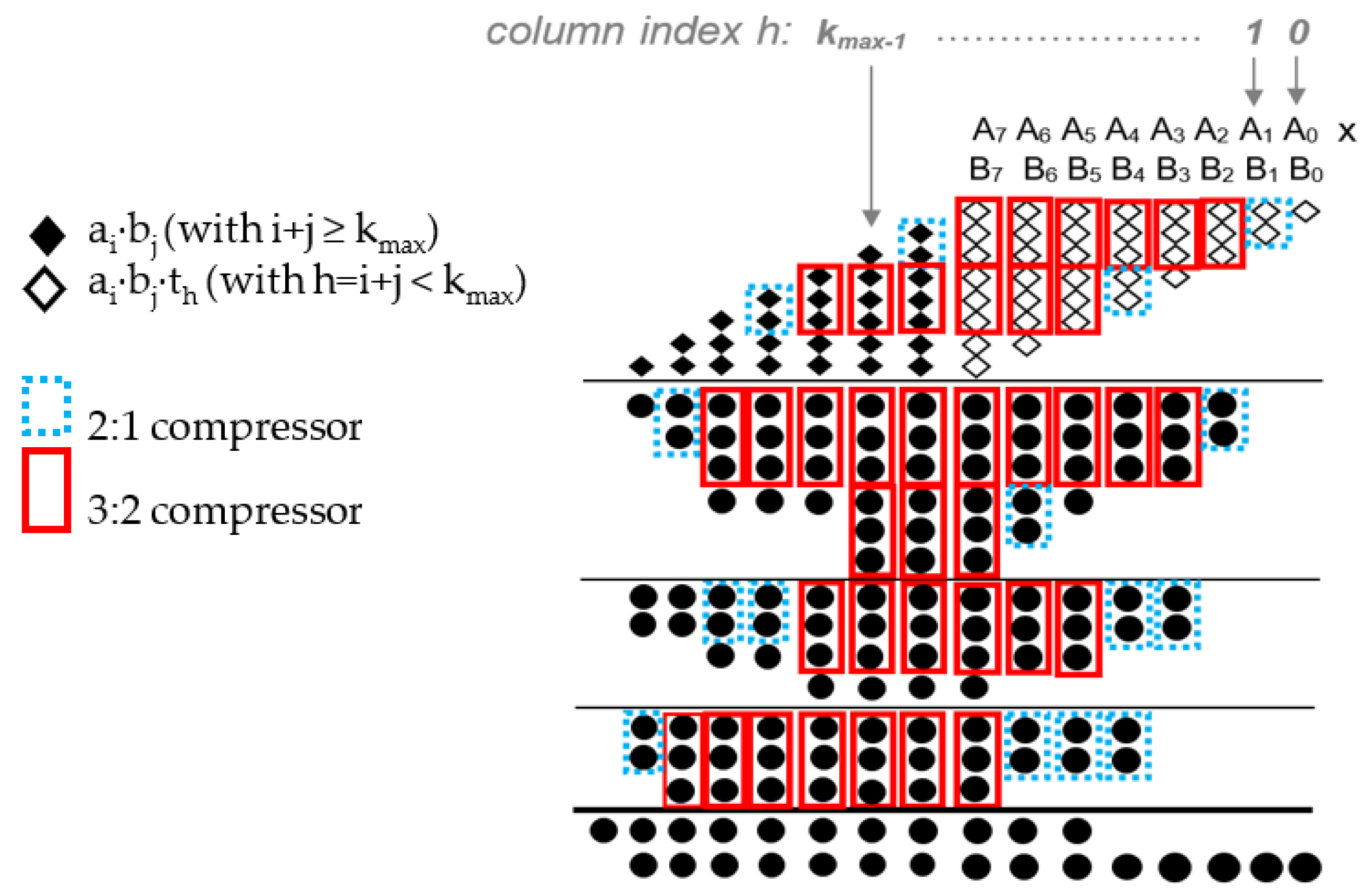
The dynamic column truncation is described in [5,6]. Here, the multiplier’ energy-quality trade-off is tuned by nullifying the switching activity of the compressors in the partial-product reduction stage belonging to a selected number of least-significant columns. With k_max being the maximum number of columns that can be truncated, all the 2-input AND gates typically employed in the multiplier partial-product generation stage and belonging to the least k_max columns are replaced with 3-input AND gates. With A_[n−1] and B_[n−1] being the two n-bit multipliers’ inputs, the (i, j)-th 3-input AND gate computes $A_i·B_j·t_h$, with $h=i+j$ and $0\le h<k_{max}$, where the control signal $t_h$ drives all the AND gates in the h-th column. The value of the control signals dictates the number of truncated columns. If $N_T<k_{max}$ columns need to be truncated, the signals $t_h$ are set as described in Equation (1):

$$t_h=\{\begin{array}{c}0, for 0\le h<N_T\\ 1, for N_T\le h<k_{max}\end{array}$$

(1)

In this way, all the bits of the partial products belonging to the least $N_T$ columns are set to 0 regardless of the value of A and B. Therefore, the switching activity of the following compressors employed in the partial-reduction stage of the multiplier and belonging to the least $N_T$ columns is zero, and the multiplier energy consumption is reduced. The value of $N_T$ entails the energy-quality trade-off: the higher (lower) the $N_T$, the lower (higher) the energy consumption and the result accuracy. Figure 1 depicts the principle of the dynamic column truncation technique applied to an 8 × 8 Wallace multiplier. In the same way as described in [10], different values of the control signal $t_h$, corresponding to a number of predetermined allowed accuracy configurations, can be stored in a ROM-based table and inputted to the multiplier according to the desired energy-quality trade-off.

All the above-described techniques plan to add a correction factor that depends on the adopted accuracy configuration. Its value is chosen at design time and it is found through an error analysis of the approximate multiplier considering a particular statistical distribution of the inputs A and B, typically supposed to be uniformly distributed.

The following section presents a possible approach to update the correction factor at runtime that is particularly suitable when the inputs are spatially and/or temporally correlated, as usually occurs in error-tolerant applications such as image processing [18].

3. The Proposed Technique and Motivation

Dynamically configurable approximate multipliers can be smartly used in error-tolerant applications whose data show spatial and/or temporal correlation. Figure 2 depicts the proposed methodology. Let us consider an input stream incoming to one of the multipliers’ input port. We can suppose that the other multiplier’s input port is receiving some coefficients (e.g., in the typical convolutional operation [9]) or another input stream (e.g., in image multiplication [7]). Each input is labeled with an increasing number according to its arrival order. As an example of application, we can suppose that each input is a pixel of an image or video frame that is scanned in raster order. The computational task requires an elaboration that may involve the single input and/or a group of its neighbors. The conventional approach consists in setting the quality level of the approximate multiplier and processing the stream one input at a time. Possibly, the approximation mode can be changed during the task execution if required by the particular context of the running application. The approximation level also dictates the value of the correction factor, which is typically found by an offline statistical analysis of the multiplier based on a supposed input distribution.

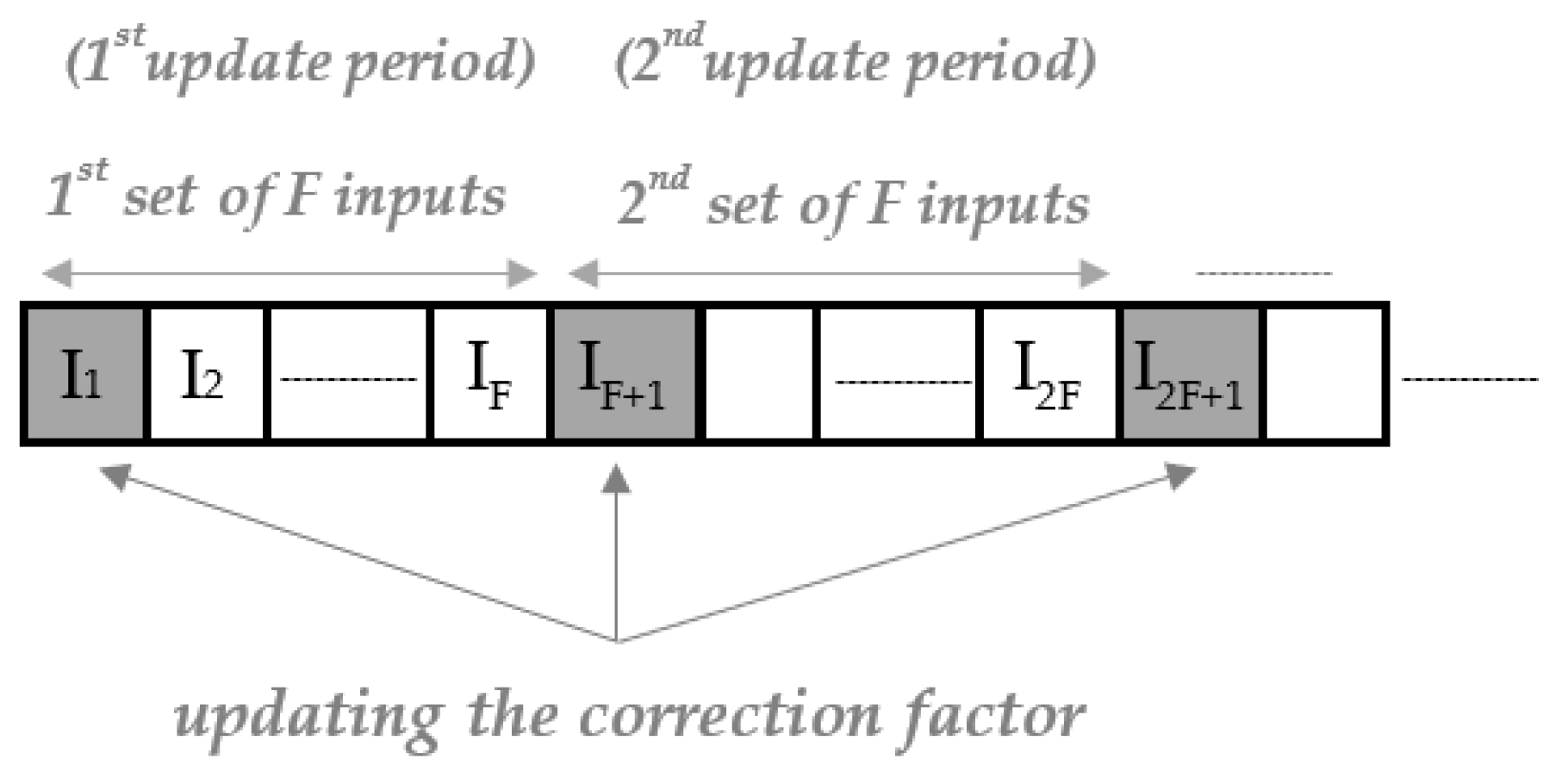
The proposed approach consists in updating the correction factor dynamically with an update period that can be tuned according to the energy-quality requirements. In Figure 2, the update period is indicated with F, which is defined as the number of consecutive inputs between two consecutive updates. The inputs involved in the updating processes are highlighted in grey. The dynamic configurability of approximate multipliers, such as in [5,6,10,17], can be exploited to periodically calculate the correction factor. A possible strategy can consist in performing two computations on the inputs highlighted in grey in Figure 2 and labeled with In_(i−1)F+1, with i being the index of the updating period, one selecting an appropriate approximation threshold and the other one selecting the accurate mode. This is possible since the selected multipliers can dynamically switch among different accuracy configurations. The difference between the results of the two computations can be used as a correction factor for the following F − 1 multiplication.

The proposed strategy is motivated by the fact that input data show a temporal/spatial correlation in typical error-tolerant applications, such as image processing. In such a case, the exact correction factor found for the input In_(i−1)F+1 can also be applied to the following inputs belonging to the same update period, with a reasonable degree of accuracy. Obviously, such a property cannot be strictly demonstrated since the scenario depends on the actual image being processed, but a useful insight can be drawn by an analysis of some benchmarks that are often used to evaluate image processing techniques [19]. 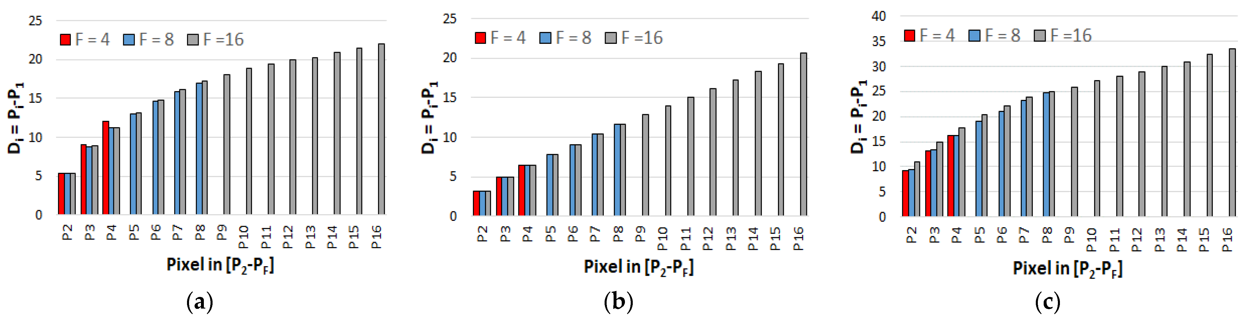Figure 3 depicts an analysis performed on three 512 × 512 8-bit grayscale benchmark images: airplane, lake and dark woman. Each image row has been divided into groups of F consecutive pixels (P₁, P₂, …, P_F), with F = 4, 8 and 16. In the histograms of Figure 3, D_i denotes the average difference between the values of pixels P_i and P₁, with i = 2 … F.

Intuitively, pixels that are spatially close to each other have a similar value, whereas the higher their distance, the higher their difference. To further analyze the proposed approach, let us consider the simple multiplication operation between the pixel P_i within the interval (P₁, P₂, …, P_F) by a constant m. The error obtained on the i-th multiplication can be expressed by Equation (2):

$${\epsilon }_i=m·P_i-\widetilde{m·P_i}$$

(2)

where $m·P_i$ and $\widetilde{m·P_i}$ are the exact and the approximate results, respectively. According to the proposed approach, the correction factor, CF, is calculated as:

$$CF=m·P_1-\widetilde{m·P_1}$$

(3)

The correction factor is then added to the results of all the F multiplications and the i-th error becomes:

$${\epsilon }_i=\{\begin{array}{c}0\\ m·P_i-\left[\widetilde{m·P_i}+m·P_1-\widetilde{m·P_1}\right]\end{array} \begin{array}{c}i=1\\ i\in \left[2, \dots ,F\right]\end{array}$$

(4)

From Equation (4), it can be deduced that a possible case when ${\epsilon }_i\to 0$ is $F\to 1$. This corresponds to update the correction factor for each P_i, which implies an exact multiplication for each input. Obviously, such a scenario is not practical since it does not consider the energy benefits of the approximate computing paradigm. On the other hand, ${\epsilon }_i\to 0$ also when $P_i\to P_1$. This case occurs when the value of the generic input, $P_i$, differs from the value of input P₁ by a very small amount. This is the scenario of typical error-tolerant applications, such as image processing depicted in Figure 3. Clearly, the condition $P_i\to P_1$ depends on the value of F: as revealed in Figure 3, the higher the F value, the smaller the probability that the input P_i may have a value close to the one of P₁. The value of F can be used as a further knob to tune the energy-quality trade-off. Indeed, the lower the F value, the higher the probability to have $P_i$≈$P_1$ and a smaller ${\epsilon }_i$. However, a low value of F entails a more frequent correction factor updating and, hence, a higher number of exact operations, and this results in a higher energy consumption.

Updating the correction factor as described in Figure 2 requires two operations on the input In_(i−1)F+1, an exact and an approximate one. This implies that the input streaming has to be stalled after each window of F inputs to perform such a double operation. For small values of F, this drawback may not be tolerable. Moreover, performing two operations for the same input obviously entails an extra energy consumption. 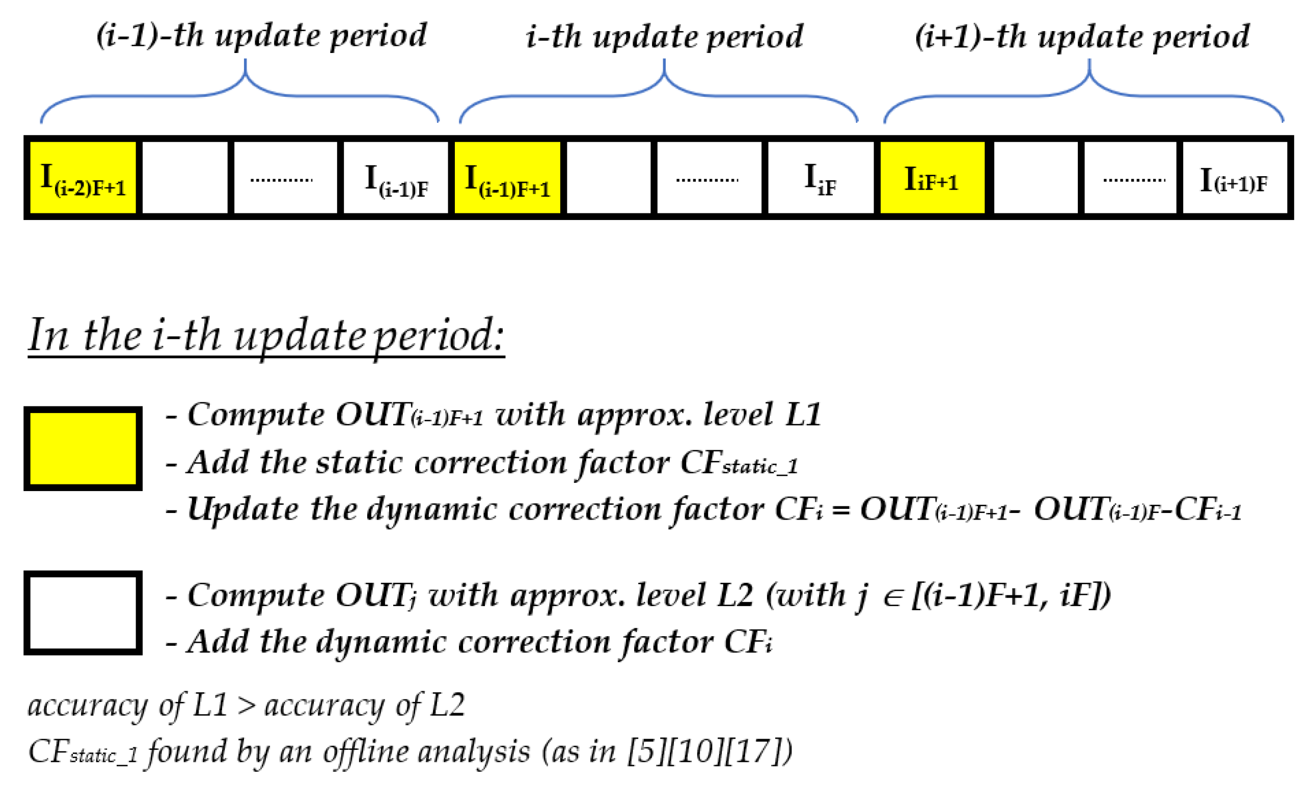In order to overcome the above-mentioned limitations, the approach described in Figure 2 can be simplified as follows:

Simplification (1): the correction factor for the i-th interval CF_i can be calculated as the difference between the result of the exact computation on the input In_(i−1)F+1 and the result of the approximate one on the previous input In_(i−1)F.

In order to exploit the spatial/temporal locality of input data, the result of the approximate computation on In_(i−1)F should not consider the correction factor CF_i calculated in the previous i-th interval. The only exception is represented by the first input I₁, since it does not have any predecessor. Consequently, a double computation is required just for I₁, thus the resulting drawbacks can be well-tolerated. Finally, the proposed approach can be further simplified:

Simplification (2): the computation accuracy on the input In_(i−1)F+1 can be relaxed.

Indeed, instead of setting the multiplier to the exact operation mode, the latter can be configured with a relatively low approximate threshold. As a consequence, the accuracy of the value of CF_i+1 is lower, but, in contrast, the energy dissipation of the computation on In_(i−1)F+1 decreases. Moreover, in order to increase the result accuracy, the computation on In_(i−1)F+1 is corrected by the static correction factor, CF_static, found with an offline procedure supposing that input data are uniformly distributed, as typically performed in previous works. Ultimately, the proposed procedure can be summarized as described in Figure 4.

4. Error Analysis of the Proposed Technique

As stated in the previous sections, the proposed approach relies on the temporal/spatial correlation that is typically found in data involved in error-tolerant applications, such as images. Hence, the error performance of the new strategy cannot be analyzed by furnishing a random input sequence to the approximate multipliers, as is generally the case when the multipliers are designed for general applications [5,6,10,17]. Instead, an actual image should be used, as one of the 8-bit benchmarks analyzed in Figure 3. In the following analysis, the convolution operation between an image and a filtering kernel has been considered as representative of the typical image processing applications. Moreover, in order to draw general considerations, the coefficients of the kernel have been randomly generated in the range [−128, 127], and a signed 8 × 8 approximate multiplier has been exploited. Although the proposed strategy can be applied to any approximate multiplier whose accuracy can be dynamically tuned, for the sake of brevity, all the following considerations will be related to the approximate multiplier based on the dynamic truncation scheme [5,6]. The reason for such a choice is that the dynamically truncated multiplier has been found to have a better energy-quality performance compared to other configurable approximate multipliers, such as those based on perforation/rounding and dual-quality compressors [6]. As described in Section 2, the energy-quality trade-off of the dynamically truncated approximate multiplier can be tuned by selecting an appropriate number $N_T$ of columns to be truncated. According to the proposed strategy, the multiplier should switch between two approximate configurations, characterized by a number of truncated columns equal to $N_{T1}$ and $N_{T2}$, with $N_{T2}<N_{T1}$. With (In_(i−1)F+1, …, In_iF) being the pixels belonging to the i-th update interval, the most accurate configuration (i.e., the one with $N_{T2}$ truncated columns) is selected when the convolution operation is centered on In_(i−1)F+1.

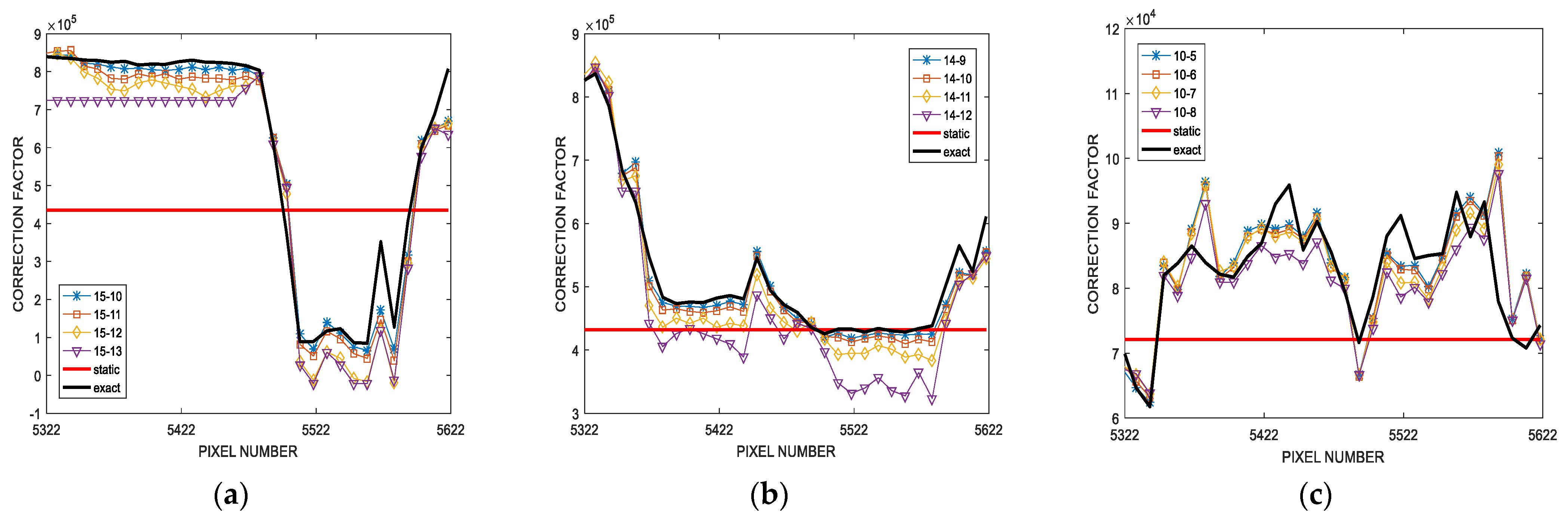
On the contrary, the more aggressive approximate configuration (i.e., the one with $N_{T1}$ truncated columns) is selected in the other cases. In the following, this configuration of the multiplier will be indicated with ($N_{T1}-N_{T2}$). Figure 5 depicts the updating of the correction factor when the proposed technique is applied to the convolution of the 512 × 512 8-bit grayscale airplane benchmark, for F = 4 and a random 7 × 7 filtering kernel. Different ($N_{T1}-N_{T2}$) multiplier configurations have been analyzed and the correction factor found by the proposed procedure (CF_dyn) has been compared with the exact (ideal) correction factor (CF_exact) and the one obtained by the typical offline error analysis (CF_static), supposing $N_{T1}$ truncated columns in both cases. For the sake of clarity, Figure 5 shows the results obtained for a randomly selected group of 300 consecutive pixels of the output image. It is worth noting that CF_dyn results to be much more accurate compared to CF_static. In particular, it is clearly visible that the behavior of CF_dyn tends to follow the same outline shown by CF_exact. Consequently, the proposed correction strategy is able to adapt itself to the actual distribution of the input data. On the contrary, the value of CF_static is always the same for all the computed convolutions, thus resulting very different from CF_exact in many cases. 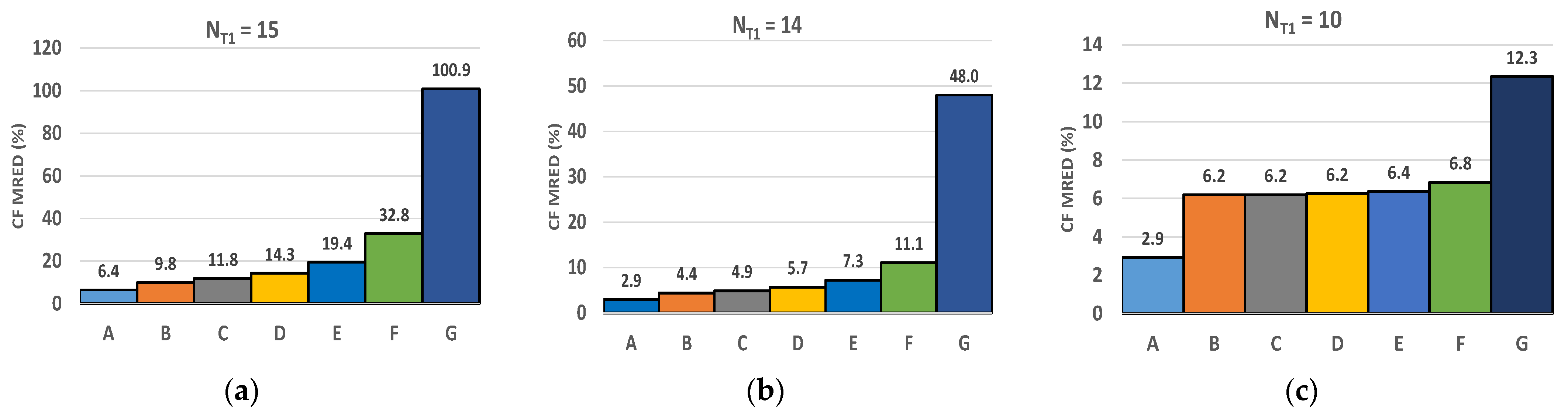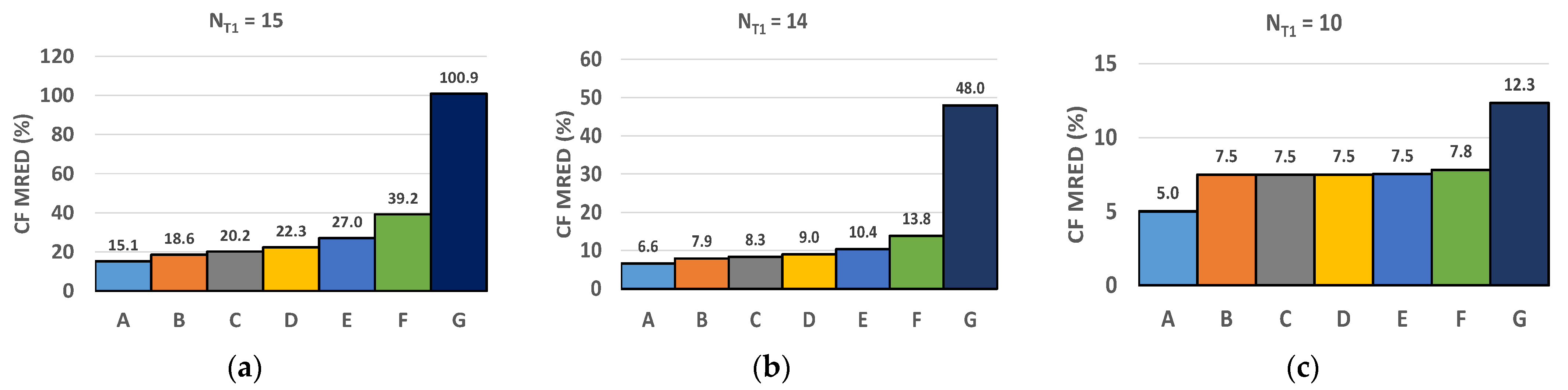Figure 6 depicts the mean relative error distance (MRED) of the correction factor, i.e., the average value of the percentage errors $\frac{\left|C{F}_{exact}-C{F}_{dyn}\right|}{\left|C{F}_{exact}\right|}$ and $\frac{\left|C{F}_{exact}-C{F}_{static}\right|}{\left|C{F}_{exact}\right|}$ calculated over all the pixels of the whole 512 × 512 filtered output. It is worth noting that the proposed technique greatly reduces the MRED of the correction factor compared to the conventional static correction procedure. As an example, such a reduction is almost 90%, for N_T1 = 15, F = 4 and the multiplier configuration set to (15, 10). Another interesting consideration can be drawn from the analysis of Figure 6: as N_T1 decreases, the MREDs of CF_dyn and CF_static tend to be equal. This consideration suggests that the proposed dynamic correction strategy is more suitable when an aggressive multiplier approximation, and hence energy-saving configuration, is enabled. Therefore, the proposed technique represents an effective way to make the quality degradation of the dynamically configurable approximate multiplier more graceful. Figure 6 also demonstrates the validity of simplifications (1) and (2) described in Section 3. Indeed, let us focus on the bars labeled with A and B in Figure 6. The bar A refers to the case when the new value of CF_dyn for the i-th update period is calculated by two operations on the input In_(i−1)F+1, an exact and an approximate one. The bar B, instead, is the result of adopting simplification (1), i.e., the new value of CF_dyn for the i-th update period is calculated as the difference between the result of the exact computation on the input In_(i−1)F+1 and the result of the approximate one on the previous input In_(i−1)F. It is worth noting that simplification (1) leads to an increase of the MRED of CF_dyn that is always lower than 3.5%. Moreover, simplification (2) also seems to be well-justified. Indeed, relaxing the accuracy of the convolution centered on In_(i−1)F+1 leads to an increase of the MRED of CF_dyn. However, such a percentage error can be tuned by varying the value of N_T2: as an example, setting N_T2 = N_T1 − 5 entails a percentage error increase that is not higher than 2%, in comparison with the ideal case N_T2 = 0 (exact computation).

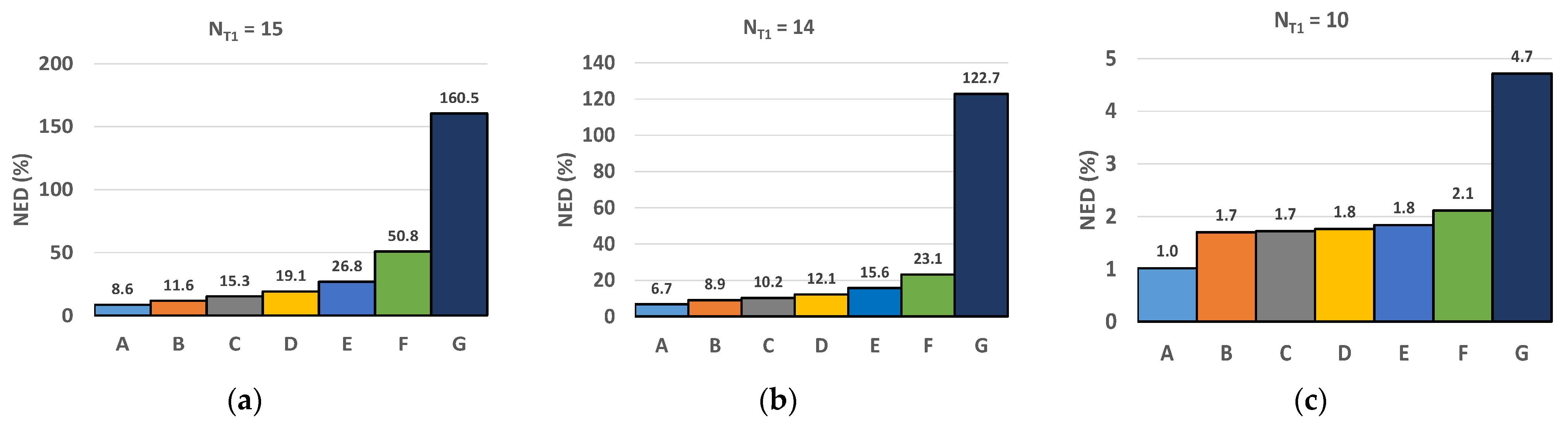
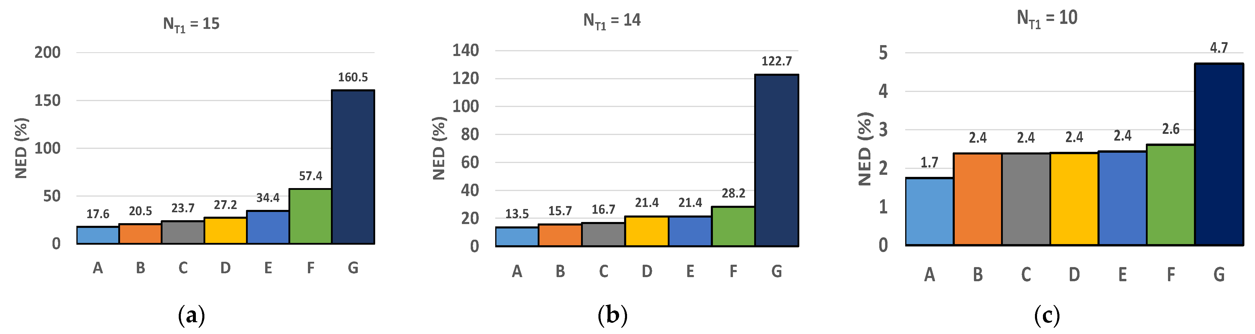
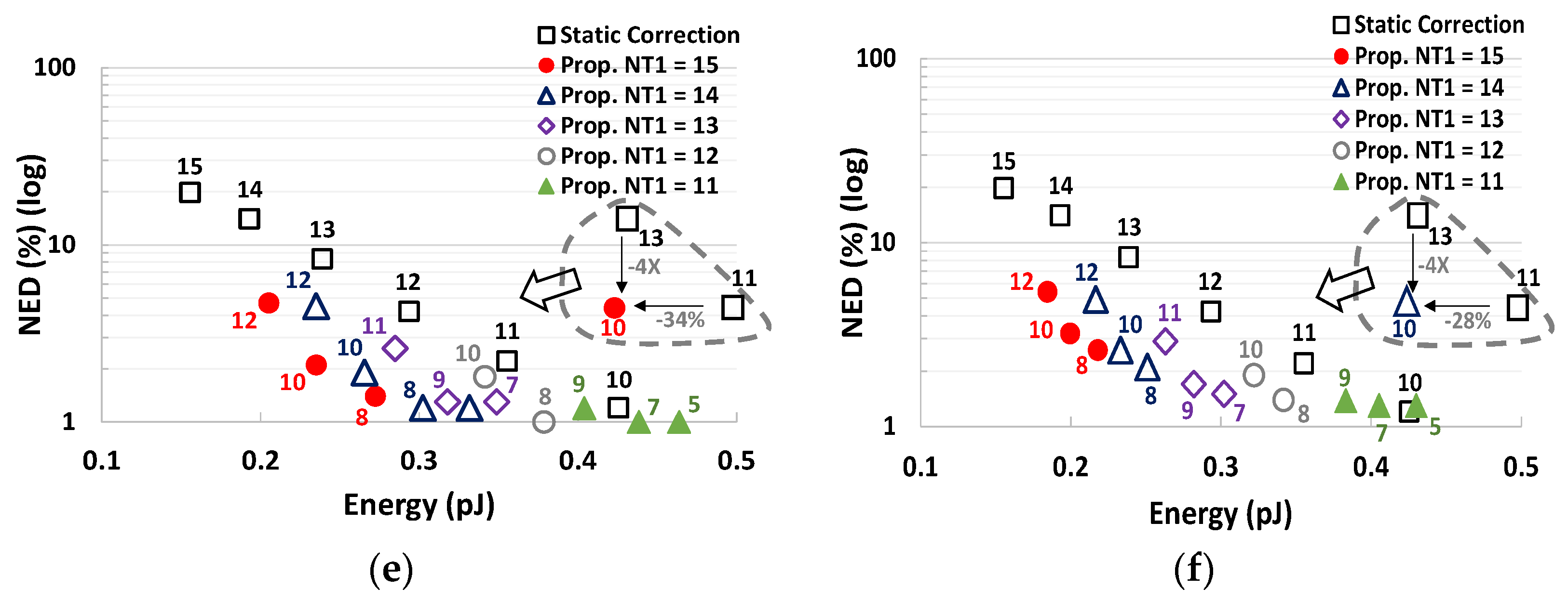
Figure 7 shows the normalized error distance (NED) [17] defined by Equation (5), with N being the pixels’ number, Out_max is the maximum value of the output pixels, and Out_i and $\widetilde{Out}$_i are the exact and the approximate i-th output pixel, respectively:

$$NED (\%)=\frac{1}{N}·{\displaystyle \sum }_{i=1}^N\frac{\left|Ou{t}_i-\widetilde{Ou{t}_i}\right|}{Ou{t}_{max}}$$

(5)

The effectiveness of the proposed approach is clearly visible since it can reduce the NED by more than 140% in comparison with the standard static correction strategy. Moreover, the validity of the proposed design simplifications is also confirmed. Indeed, simplification (1) leads to a maximum NED increase of only 3%, whereas adopting simplification (2) entails an extra NED increase that can be lower than 4%, in conjunction with a tuning of the value of N_T2. The above-described analysis has also been carried out for F = 8. 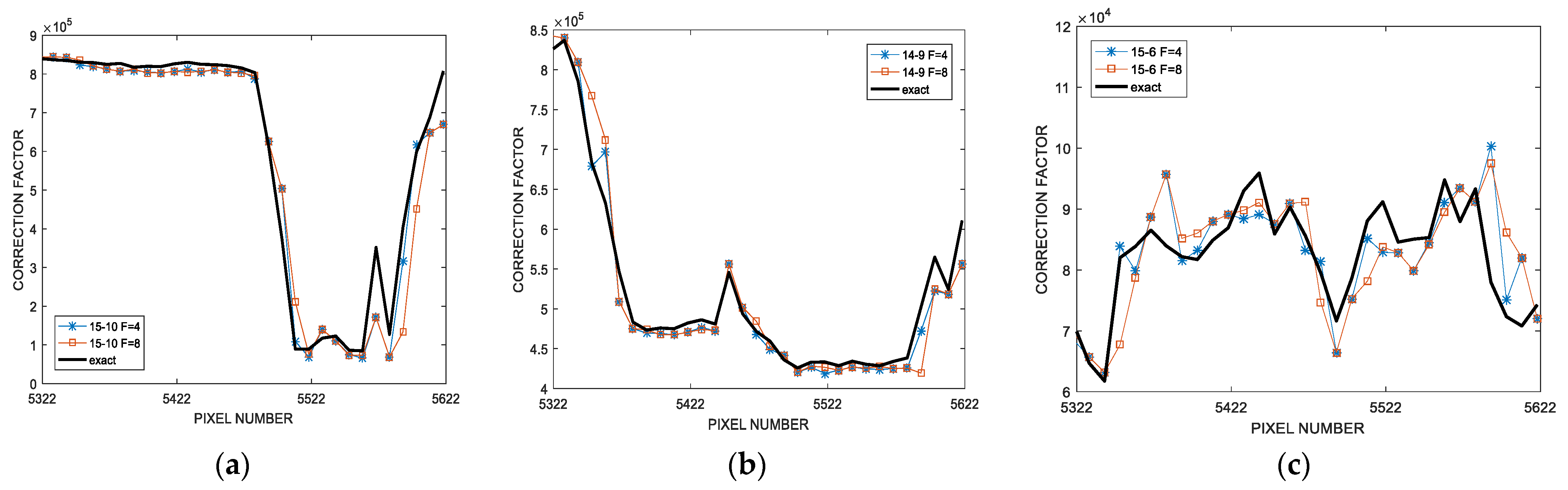Figure 8 shows the updating process of CF_dyn for F = 4 and F = 8 and several ($N_{T1}-N_{T2}$) multiplier configurations. The value of CF_dyn is further from the exact value for F = 8: this is an expected result since, as previously pointed out in Figure 3, the larger the value of F, the lower the probability that the pixels belonging to the same update window have similar values. Figure 9 and Figure 10 depict the MRED of the correction factor and the NED of the output for F = 8, respectively. It is worth noting that all the previous considerations that have been drawn for the case F = 4 are still valid. In particular, the validity of the two simplifications is also confirmed for the case F = 8. As expected, the CF MRED and the output NED for the case F = 8 are higher than the values obtained for F = 4; as discussed above, this is the consequence of a larger error correction window update.

Finally, the effect of the kernel size has also been investigated.

Table 1. 3 × 3 convolution.

Error NED (%)
Configuration	F = 4			F = 8
	NT1 = 15	NT1 = 14	NT1 = 13	NT1 = 15	NT1 = 14	NT1 = 13
A	9.8	7.7	1.6	18.4	13.2	2.3
B	13.6	10.3	2.7	21.2	15.4	3.4
C	16.8	11.5	2.7	24.1	16.4	3.4
D	19.4	13.4	2.8	26.4	18.1	3.4
E	25.1	15.8	2.8	31.9	20.2	3.4
F	34.9	21.15	3	41.1	25.1	3.5
G	116	79.5	4.4	116	79.5	4.4
CF MRED (%)
Configuration	F = 4			F = 8
	NT1 = 15	NT1 = 14	NT1 = 13	NT1 = 15	NT1 = 14	NT1 = 13
A	22.7	9.5	7.3	42	16	10.4
B	35.5	14.4	15.3	51.6	20.2	16.8
C	38.5	15.3	15.3	53.7	20.8	16.7
D	41.4	16.7	15.4	55.8	21.8	16.7
E	47.1	18.8	15.5	60.8	23.5	16.8
F	59.6	23.3	15.9	71.2	27.4	16.9
G	137.5	62.1	17.6	137.5	62.1	17.6

summarizes the MRED of the correction factor and the output NED obtained when a 3 × 3 kernel with randomly generated coefficients in the range [−128, 127] has been used for the convolution. The meaning of the configurations in the first column of Table 1 is the same as described in the caption of Figure 6. Additionally, for the 3 × 3 convolution kernel, the proposed approach has shown significant advantages compared to the conventional solution with a constant correction factor. In particular, the proposed dynamic approach is able to reduce the MRED of the correction factor and the output NED (configuration A with N_T1 = 15 and F = 4) by up to 100%. As expected, the lower the N_T1 and/or F, the higher the accuracy.

5. The Gaussian Filter as a Case Study: Quality Results

In this section, a typical image processing application, i.e., the Gaussian filter [9], is taken as a reference and the quality results deriving from the application of the proposed methodology are investigated. The 7 × 7 Gaussian filter used is described in Equation (6):

$$\mathrm{K}=\frac{1}{4096}\left[\begin{array}{ccccccc}1& 6& 15& 20& 15& 6& 1\\ 6& 36& 90& 120& 90& 36& 6\\ 15& 90& 225& 300& 225& 90& 15\\ 20& 120& 300& 400& 300& 120& 20\\ 15& 90& 225& 300& 225& 90& 15\\ 6& 36& 90& 120& 90& 36& 6\\ 1& 6& 15& 20& 15& 6& 1\end{array}\right]$$

(6)

Quality results have been obtained by modeling the filtering operation of Equation (6) in Matlab, taking typical 8-bit 512 × 512 greyscale images as benchmarks [19]. Figure 11 depicts the peak-to-noise ratio (PSNR) and the structural similarity index metric (SSIM) of the filtered images for F = 4 and F = 8 respectively, averaged on three benchmarks: lake, dark woman and airplane. The analysis has been carried out by varying several multiplier parameters: the number of truncated columns (N_T) for the standard approach (static correction factor), and the number of truncated columns in the lower accuracy (N_T1) and higher accuracy mode (N_T2) for the proposed correction approach. For each value of N_T, the static correction factor related to the conventional procedure has been evaluated as the multiplier mean error obtained for 1 M uniformly distributed inputs. Several considerations can be drawn from Figure 11. Indeed, when a relatively low quality is required (PSNR < 34 dB or SSIM < 0.75), the proposed approach is able to work with N_T1 > N_T. This is preferable since the higher the number of truncated columns, the higher the energy saving. As an example, when its configuration is set to (N_T1, N_T2) = (15, 10) and F = 4, the new correction strategy leads to about the same PSNR as shown by the static correction technique for N_T = 11. As expected, the novel approach shows a quality saturation as N_T2 approaches a relatively low value, since the error correction factor does not show any further sensible accuracy increase for any further reduction of N_T2. Such a behavior is in agreement with the considerations drawn by the analysis described in the previous Section 4. Indeed, as shown in Figure 6, Figure 7, Figure 8, Figure 9 and Figure 10, when N_T2 approaches the value N_T1 − 5 (histogram bar C), the MRED of the correction factor starts to converge to the ideal value corresponding to the case N_T2 = 0 (histogram bar B). It follows that, when a higher output quality is required (PSNR > 34 dB or SSIM > 0.75), the simpler static correction technique shows quality results that are similar to those deriving from the proposed dynamic correction approach.

6. Hardware Implementation and Energy-Quality Trade-Off

The hardware implementation of the analyzed Gaussian filter is described in Figure 12. It is based on a pipelined multiply-accumulate (MAC) circuit consisting of an 8 × 9 dynamically truncated unsigned Wallace multiplier and a 20-bit ripple carry adder (RCA)-based accumulator needed to accumulate the 7 × 7 multiplications of the filter described in Equation (6). The final accumulation is right-shifted by 12-bit positions to perform the division by 4096 and to obtain the final 8-bit filtered pixel. The circuit highlighted in red aims at updating the correction factor CF_dyn periodically, as described in Section 3. Since the first pixel of each image row has no predecessor, we adopted the strategy to perform two computations on it, one with lower accuracy and the other with higher accuracy, and to obtain the first correction factor by the difference of the two results. A finite state machine (FSM) provides the multiplexers’ selection signals, C1–C4, and the truncation signals, th, to the multiplier, according to the definition of Equation (1). In the following, there is a description of the computational steps consecutively performed by the proposed hardware implementation.

(a) Low-accuracy convolution centered on the first pixel of the first row: At the beginning of the convolution, the signal C3 is set to ‘0’, so that the register Corr. Reg. is initialized at 0, and the signals C4 and C2 are set to ‘1’ and ‘10’ respectively, in order to add a zero constant to the first accumulation. The signal C1 is set to ‘1’ in order to freeze the dynamic switching activity of the correction factor updating circuit to save power. Moreover, the FSM sets the signal th to the value th_NT1, corresponding to a number of truncated columns, N_T = N_T1 (lower accuracy). Such a value is supposed to be stored in a register. After the first accumulation, the signal C2 is set to ‘00’ to enable the accumulation feedback. In this way, the value of CF_dyn obtained after the 7 × 7 MAC operations coincides with the first 8-bit filtered pixel at lower accuracy. We will refer to this value as OUT_{1_LA}. After the conclusion of the last accumulation operation, the signals C1 and C3 are set to ‘0’ and ‘1’ respectively, for one clock cycle, so that the value OUT_{1_LA} can be stored into Corr. Reg.

(b) High-accuracy convolution centered on the first pixel of the first row: The 7 × 7 convolution centered on the first pixel of the first row is repeated at the higher accuracy. Towards this aim, the signal th is set to the value th_NT2, corresponding to a number of truncated columns, N_T = N_T2 (higher accuracy). Such a value is supposed to be stored in a register. The signals C4 and C2 are set to ‘0’ and ‘10’ respectively, in order to add the value of the static correction factor, CF_stat, corresponding to N_T = N_T2 and loaded in advance into a register, to the first accumulation. After the first accumulation, the signal C2 is set to ‘00’ to enable the accumulation feedback. For the whole duration of the 7 × 7 convolution computation, the signals C1 and C3 are set to ‘0’ and ‘1’ respectively, in order to save power, and the register Corr Reg. is clock-gated in order to keep the previous stored value OUT_{1_LA.} At the end of the final accumulation operation, the output coincides with the 8-bit filtered pixel at higher accuracy (let us indicate this value, OUT_{1_HA}). The signals C1 and C3 are set to ‘0’ and ‘1’ respectively, for one clock cycle, and the clock gating on register Corr. Reg. is disabled, also for one clock cycle: the value of the signal CF_dyn is hence calculated as OUT_{1_HA} − OUT_{1_LA} and stored in Corr. Reg.

(c) Low-accuracy convolution centered on the following F − 1 pixel: After the computation of the last accumulation operation at the higher accuracy, the convolution centered on the second pixel has to be computed. As a consequence, the signal CF_dyn is forwarded to the accumulation feedback by setting the signal C2 to ‘01’ for one clock cycle. Hence, the correction factor, CF_dyn, is added to the following accumulation operation. At the same time, the multiplier lower-accuracy mode is enabled by setting the signal th to the value th_NT1, corresponding to a number of truncated columns, N_T = N_T1 (lower accuracy). As described in the previous points, after the first accumulation, the signal C2 is set to ‘00’ to enable the accumulation feedback. For the whole duration of the 7 × 7 convolution computation, the signals C1 and C3 are set to ‘0’ and ‘1’ respectively, in order to save power, and the register Corr Reg. is clock-gated in order to keep the previous stored value CF_dyn. This same control strategy is perpetuated for the convolutions centered on the following pixels belonging to the same update period. The only exception is represented by the control signal C2, which is set to ‘11’ for one clock cycle at the beginning of a new convolution; in this way, the value of the correction factor can be inserted in the accumulation feedback directly from the output signal, CF_{dyn_reg}, of the register Corr. Reg.

(d) Updating the value of the register Corr. Reg.: The content of the register Corr. Reg. has to be updated at the end of the convolution operation centered on the F-th pixel, i.e., the last pixel of the first update period. To this aim, the update correction circuit is enabled by setting the signals C1 and C3 to ‘0’ and ‘1’ respectively, for one clock cycle, an disabling the clock gating on the register Corr. Reg. for one clock cycle. Let us indicate with (OUT_{F_LA})_corr the (corrected) value of the F-th 8-bit filtered pixel computed at the lower accuracy. The register Corr. Reg. is then updated with the value OUT_{F_LA} = (OUT_{F_LA})_corr − CF_dyn, i.e., the value of the F-th 8-bit filtered pixel without considering the correction factor. This is exactly what is requested by the proposed update strategy depicted in Figure 4.

(e) Updating the correction factor: As depicted in Figure 4 (yellow step), the convolution centered on the following (F + 1)-th pixel has to be performed at the higher accuracy. Therefore, the MAC is configured again as described in point (b). At the end of the last accumulation of the (F + 1)-th convolution, the signals C1 and C3 are set to ‘0’ and ‘1’ respectively, for one clock cycle, and the clock gating on register Corr. Reg. is disabled, also for one clock cycle. The value of the signal CF_dyn is hence updated with the value OUT_{F+1_HA} − OUT_{F_LA} and stored in Corr. Reg. The described procedure is then repeated starting from point (c) until the end of the image row.

At the beginning of each new image row, the computational steps (a)–(e) start again. The timing with which the FSM provides the described control signals is regulated by three counters, advising the time when a 7 × 7 convolution ends (signal TW), when an update period finishes (signal TF) and when the computation of the entire image row has been completed (signal TR). Finally, the designed hardware architecture has been enriched with the possibility to also work according to the conventional static correction strategy. Indeed, as pointed out at the end of Section 5, the quality results of the latter configuration are similar to those obtained by the proposed methodology for a relatively low value of the parameters N_T and N_T1. This occurs because the error becomes very low so the static approach can assure a high accuracy by itself. In such a situation, the static approach is preferable because it does not entail the energy drawbacks of a more accurate computation, as required by the proposed technique. The input dyn configures the MAC to work according to either the proposed dynamic correction updating strategy (dyn = 1) or the conventional static correction approach (dyn = 0). When dyn = 0, the FSM always sets the control signal C4 to ‘0’ and the signal th to th_NT2.

The architecture of Figure 12 has been described in Verilog and synthetized with Cadence Genus, exploiting the ST 28 nm UTBB FDSOI technology. The 12-track 1 V Typical Process Regular Threshold Voltage (RTV) Standard Cell library has been adopted in all the implementations. The same MAC version based only on the usual static correction approach has been taken as a reference design. Obviously, the latter does not employ the FSM and the correction updating circuit, but only the counter for the signal TW is needed. The dynamically truncated approximate multiplier and the adders have been described in Verilog in a structural way. For the multipliers, the Wallace scheme with 3:2 (Full-Adder) and 2:1 (Half-Adder) compressors has been adopted in the partial reduction stage. For the sake of a low energy consumption, each designed multiplier adopts a ripple carry adder (RCA) as a final carry propagate adder. For the same reason, the accumulating adder of the MAC and the subtractor in the correction factor updating circuit have also been described according to the RCA structure. The minimum delay for both the designs has been found to be 460 ps (limited by the multiplier, which is the same for both the implementations), whereas the proposed methodology entails +43% more area. Both the designs employ clock gating to save dynamic energy on those Flip-Flops in the pipeline that can stay idle depending on the multiplier truncation configuration (clock gating latches are not shown in Figure 12).

Table 2. Energy dissipation (pJ) of the standard and proposed designs.

Accurate MAC
	Mult	Adder	Err. update	clk	FSM	Gating latches	Counter	Other	Total
	0.458	0.248	-	0.092	-	-	0.032	0.013	0.844
Standard static correction approach
NT	Mult	Adder	Err. update	clk	FSM	Gating latches	Counter	Other	Total
10	0.191	0.091	-	0.080	-	0.018	0.032	0.013	0.426
11	0.142	0.075	-	0.075	-	0.018	0.032	0.013	0.355
12	0.102	0.058	-	0.069	-	0.018	0.032	0.013	0.293
13	0.069	0.044	-	0.062	-	0.018	0.032	0.014	0.239
Proposed (F = 4, NT2 = NT1 − 5)
NT1	Mult	Adder	Err. update	clk	FSM	Gating latches	Counter	Other	Total
13	0.126	0.063	0.004	0.068	0.005	0.017	0.037	0.013	0.334
14	0.094	0.050	0.004	0.061	0.005	0.017	0.037	0.013	0.281
15	0.066	0.039	0.004	0.054	0.005	0.017	0.037	0.013	0.235
Proposed (F = 8, NT2 = NT1 − 5)
13	0.098	0.056	0.002	0.065	0.005	0.016	0.036	0.013	0.290
14	0.070	0.042	0.002	0.057	0.005	0.016	0.036	0.013	0.240
15	0.045	0.033	0.002	0.049	0.005	0.016	0.036	0.013	0.198

reports the average energy dissipation per operation of the two designs for a few truncation configurations, obtained from back-annotated simulations at the maximum clock frequency, based on the image benchmarks reported in the previous section. The energy dissipation has been separated into the components related to the multiplier, the adder, the FSM, the correction factor updating circuit, the clock gating latches, the clock network and the counters. The average energy dissipation per operation of each MAC implementation has been found by multiplying the average power consumption (estimated by the Cadence Genus tool by means of .vcd files coming from back-annotated simulations) by the clock period.

As expected, the MAC average energy dissipation per operation increases as N_T and N_T1 decrease. For the proposed approach, a higher value of F leads to a lower MAC energy dissipation because the time when the MAC is configured with a lower accuracy is larger. Moreover, the lower the N_T and N_T1, the higher the clock network energy dissipation because, as the number of truncated columns decreases, the number of clock-gated FFs decreases as well. The energy overhead of the extra counters is insensitive to the value of N_T1, whereas it slightly depends on F. Compared to the single counter of the standard static correction approach, the extra counters needed by the proposed dynamic approach entail 15.6% (12.5%) more energy for F = 4 (F = 8). As expected, the higher the value of F, the lower the energy dissipation of the correction factor updating circuit. This is reasonable since a higher value of F means a lower activity for the circuit. In particular, from Table 2, it can be easily inferred that the energy dissipation of the correction factor updating circuit is halved when the value of F doubles. Anyway, the extra energy dissipation of the correction factor updating circuit and extra counters represents a very small percentage of the total energy dissipation: up to 3.8% and 3% for F = 4 and F = 8, respectively. It is worth noting that the accurate MAC has a slightly lower minimum clock period constraint (447 ps), 2.8% lower than the delay of the proposed design, since the partial product generation stage of the accurate multiplier exploits 2-input AND gates rather than 3-input AND gates. Moreover, the area overhead of the proposed design with respect to the accurate one is about 46%, since the latter does not need clock gating latches. The energy consumption of the MAC designed according to the proposed approach is up to 72% and 76% lower with respect to the accurate MAC for F = 4 and F = 8, respectively. 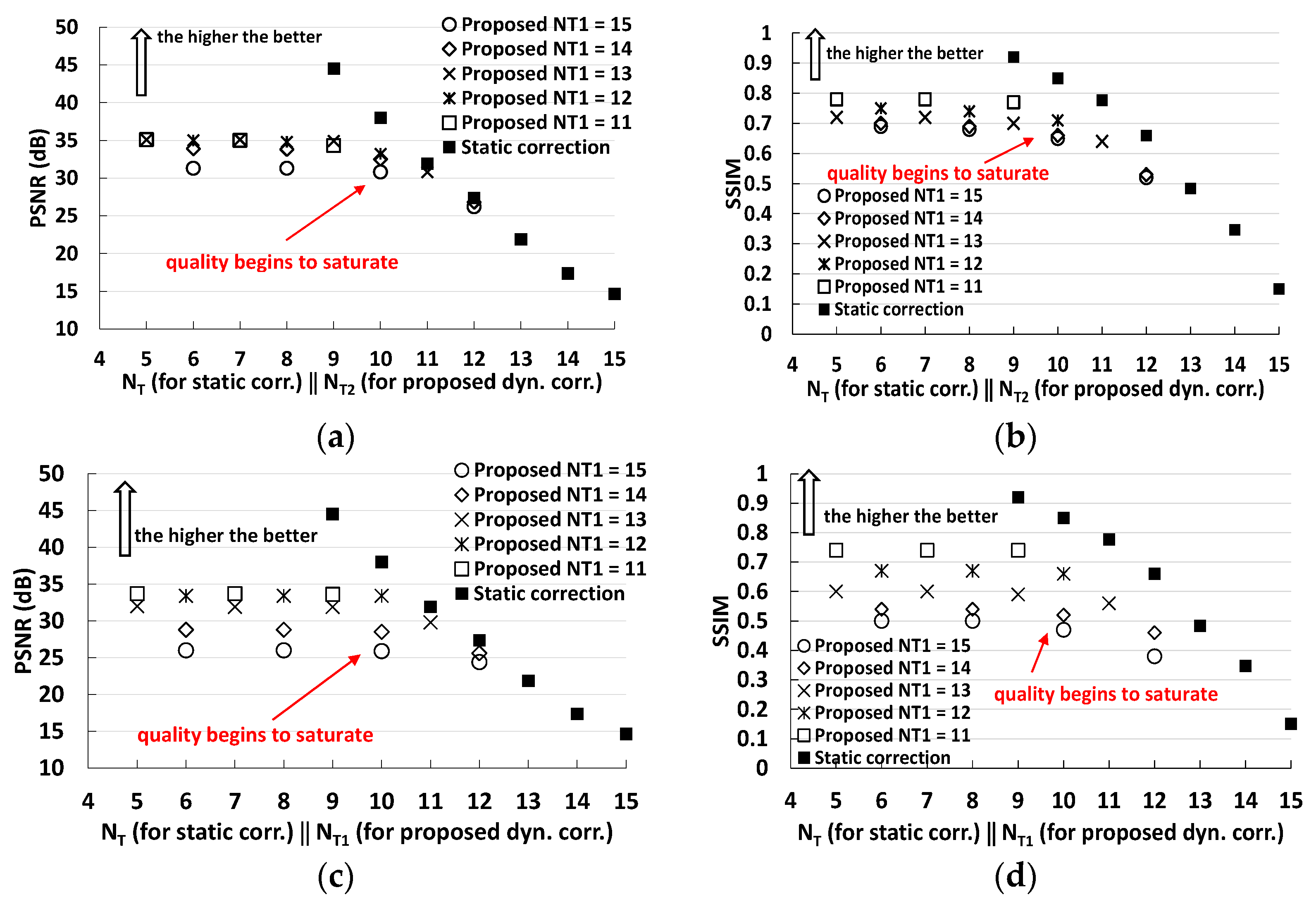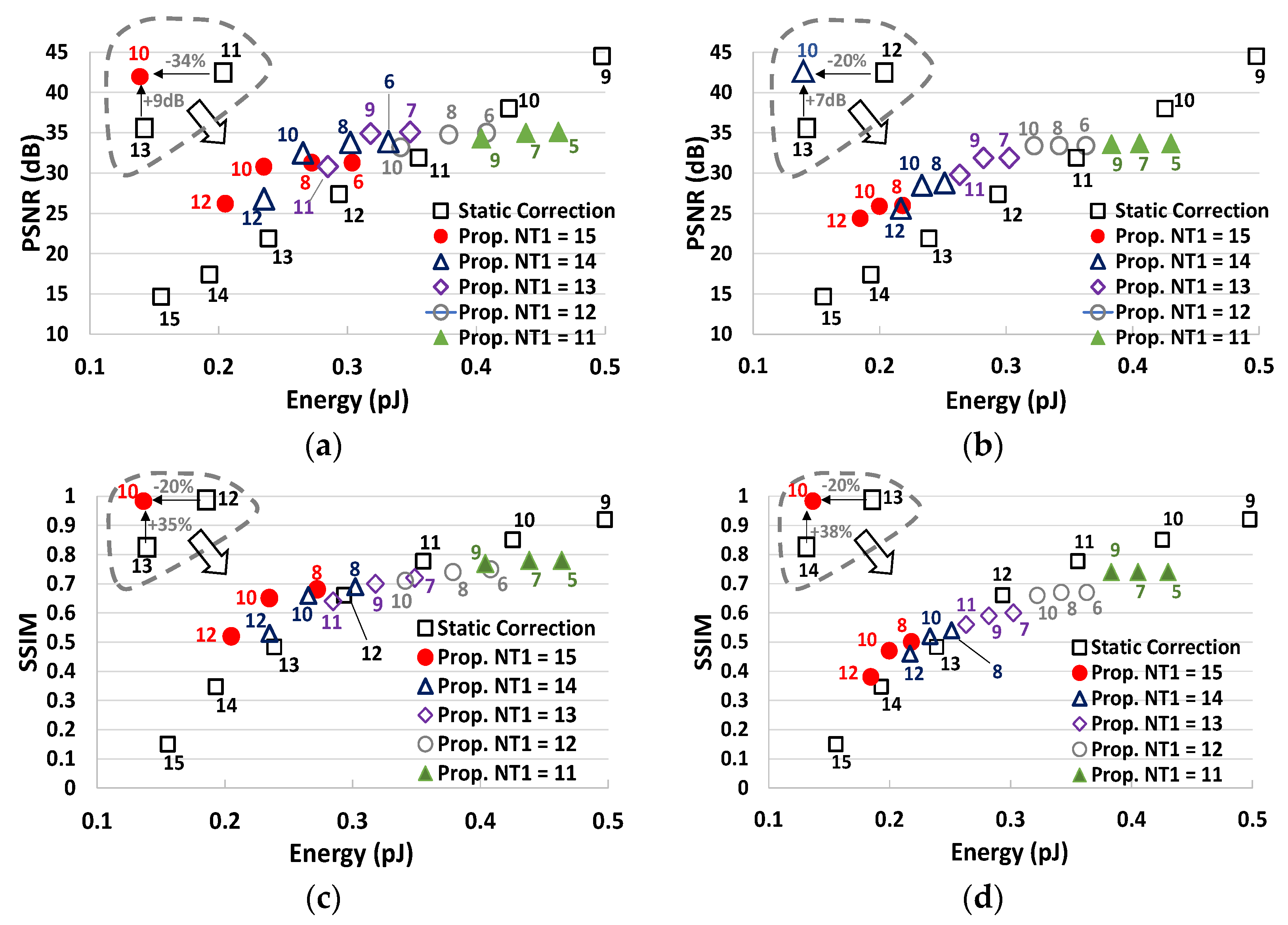Figure 13 depicts the energy-quality trade-off for the standard and proposed designs for different values of N_T1 and N_T2. The quality has been evaluated with three metrics: PSNR, SSIM and NED. As expected from the preliminary analysis of Figure 11, the proposed methodology shows a quality saturation for low values of N_T2, thus the standard approach is preferable when a higher quality is required (PSNR > 32 dB, SSIM > 0.7, NED < 1%). On the contrary, for lower-quality values, the proposed methodology shows a better energy-quality trade-off. As it is visible in the insets of Figure 13, the energy consumption is reduced by up to 34%, 34% and 20% at the parity of PSNR, NED and SSIM, respectively. Similarly, the proposed technique can improve the PSNR, the NED and the SSIM by up to +9 dB, −4× and +35% respectively, at iso-energy. The energy saving is even higher if we consider only the energy consumption of the clock network, the multiplier, the adder and the correction update circuit (when applied). Indeed, the remaining components can be shared among several MACs if the computation is parallelized. In such a scenario, the proposed design can reduce the energy dissipation by up to 44%, 44% and 29% at iso-PSNR, iso-NED and iso-SSIM, respectively. Finally, when a high quality is required, the proposed design needs to be configured to work with a constant correction factor (dyn = 0); in such a case, the proposed design has shown a negligible extra power consumption with respect to the standard design (less than 1.5%).

7. Conclusions

This paper has proposed a simple approach to improve the quality degradation of dynamically configurable approximate multipliers, exploiting the spatial and/or temporal input correlation typically shown by error-tolerant applications, such as image and video processing. By periodically changing the approximation level of the multiplier, the correction factor can be updated at runtime and adapted to the incoming inputs. When applied to a typical image processing application (the Gaussian filter), the proposed approach has shown an energy reduction of up to 34% at iso-quality and a PSNR, NED and SSIM improvement of up to +9 dB, −4× and +35% at iso-power respectively, compared to the traditional correction approach employing a static correction factor. As future works, it is planned to investigate the proposed methodology for other error-tolerant applications, such as machine learning for image/audio recognition.