An Efficient Distributed Elliptic Positioning for Underground Remote Sensing

Abstract

Remote surveying of unknown bound geometries, such as the mapping of underground water supplies and tunnels, remains a challenging task. The obstacles and absorption in media make the long-distance telecommunication and localization process inefficient due to mobile sensors’ power limitations. This work develops a new short-range sequential localization approach to reduce the required amount of signal transmission power. The developed algorithm is based on a sequential localization process that can utilize a multitude of randomly distributed wireless sensors while only employing several anchors in the process. Time delay elliptic and frequency range techniques are employed in developing the proposed algebraic closed-form solution. The proposed method is highly effective as it reaches the Cramer–Rao Lower Bound performance level. The estimated positions can act as initializations for the iterative Maximum Likelihood Estimator (MLE) via the Taylor series linearization to acquire even higher positioning accuracy as needed. By reducing the need for high power at the transmit modules in the sensors, the developed localization approach can be used to design a compact sensor with low power consumption and greater longevity that can be utilized to explore unknown bounded geometries for life-long efficient observation mapping.

1. Introduction

Freshwater supply has decreased due to the continuous waste production from industrial sewage, agriculture, and other human and animal activities. Even though around 73% of the Earth’s surface is covered with water, only about 2.1% is available freshwater [1,2]. A sufficient clean water supply is essential for producing crops, habitat conservation, soil formation, and the cycling of nutrients [1]. If drinking water is contaminated due to a biological or a chemical substance, it can lead to the formation of contagious illnesses, such as pneumonia, hepatitis, and gastric ulcers [3,4]. Lead (Pb), mercury (Hg), cadmium (Cd), and arsenic (As), and other hazardous heavy metal substances can also be found in water sources. Another area of concern in monitoring water quality is the residence of microbes in the water supply, which can expose humans and the entire water ecology to a significant danger [1]. Hence, the advancement of ultra-sensitive and rapid detection techniques is critical in effectively safeguard the available clean water supply worldwide.

During the past two decades, numerous research has been done to construct more effective methods to detect contamination with low operating costs and energy. In the past, water supply contaminants were manually detected in water laboratory sites where contamination analysis was carried out at the laboratory level [5]. Frequently used instruments in detecting contamination are capillary electrophoresis, field-flow fractionation, mass spectrometry, and multiple fermentation tube techniques [1]. Recent technological advancements in biosensor procedures and analytical chemistry improved the sensitivity and accuracy of detection assays. Some of these technological developments include water quality sensors [6], model-based event detection [7], and advanced spectroscopy [8]. Other contamination detection methods include sensor placement approach [9], Microfluidics sensors [10], biosensors [11], and light emission [12,13]. There are several types and applications of touching monitoring systems. Mobile and static sensors are employed to acquire real-time information about the underground and pipeline water supply. The mobile sensors are positioned inside the system at the starting source point and continue to migrate until the sink point has been reached. The data are stored in the memory of the mobile sensor and transmitted to the backend system (central processing system) for more advanced analysis. The collected information can be correlated with the sensor’s location to create a real-time mapping of the observations in the tested system [2]. As a real-time assessment for sampling and analysis, online sensor monitoring provides a broader data frequency than the traditional sample-based method. Additionally, online monitoring is flexible and can be conducted remotely while still retaining a faster response rate. Online monitoring systems based on Wireless Sensor Network (WSN) provide sufficient datasets, straightforward monitoring assessment, simultaneous data measurements, and higher sensitivity and detection accuracy [1]. An online monitoring system based on WSN consists of monitoring centers, base stations, and information monitoring nodes [14]. In addition, the usage of WSN lowers the consumption of power which lowers the operational cost associated with running the system [15]. The typical design of a sensor network incorporates a low-power processor, a sensor interface, and a wireless communication module [1]. Some WSN utilizations have been used in monitoring water quality [1,16]. For example, Wu et al. [17] devised a self-powered transportable sensor that detects pH and disinfectant-related ions levels in water distribution pipelines in real-time. For highly dynamic systems, such as biological and chemical contamination monitoring in underground or underwater systems with more diverse topologies, it is recommended to use a centralized processing algorithm that provides more accurate location information when compared to distributed processing algorithms [2]. The aggregated data can be used to find a time-based pattern of data distribution. The main goal of sensor distribution is to adequately cover the maximal space of the tested system (such as underground water supply). This centralized exploitation technique applies WSNs with sensors dispersed in a small area and has inadequate reliability due to loss in accumulated data resulting from multi-hop transactions [2]. Moreover, this approach requires an enormous amount of energy and bandwidth consumption [18].

The reliability of remote sensing devices depends on the lifetime requirements of different applications and the energy storage capacity of sensor nodes [19]. Therefore, a more compact sensor design with low energy consumption modules is highly appreciated for successful long-term wireless network surveillance. An efficient long-life power source is important to run the different modules in the mobile sensor (sensor interface module, actuation module, and signal transmission module). The interface and actuation systems depend on the application type and nature of the media (liquid/gas).

For successful underground explorations and remote surveillance, the wireless coverage of mobile sensors should be adequate to ensure reliable real-time connectivity. However, devices with very high-frequency (VHF)/ultra-high frequency (UHF) radio equipment may not be as effective underground as aboveground due to signal fading and high multipath propagation [20]. Theoretically, the amount of power required for successful communications between two network terminals (nodes) is equivalent to the effective aperture of the receiving antenna at a distance d from the antenna transmitting signal [21,22]. The simplest form to predict the best case received signal power is

$$P_r={\delta }_t{\delta }_r{\left({\displaystyle \frac{\lambda }{4\pi d}}\right)}^n{P}_t,$$

(1)

where: $P_t$ represents the power fed into the transmitting antenna input terminals, $P_r$ serves as the power available at receiving antenna output terminals, $\lambda$ is the wavelength of the radio frequency, n represents the path loss exponent, ${\delta }_t$ and ${\delta }_r$ are the antenna directivities of the transmitting and receiving antennas, respectively.

Many factors can cause the received signal power to be lower than the simple form of the Formula (1), such as an obstructed link due to buildings, trees, hills, earth curvature, atmospheric attenuation, and antenna misalignment [23]. By ignoring the noise and interference of the telecommunication signal and assuming that the transmitter/receiver antenna is an absorption-less medium, Equation (1) can be reduced to the following equation:

$$P_t=\left(C{P}_r\right)d^n,$$

(2)

where C is a constant that depends on the antenna directivity and the wavelength. From Equation (2), it can be concluded that the required transmission power $P_t$ is directly proportional with at least the square of the distance between the nodes’ antennas, assuming the received power $P_r$ is more than the minimum threshold power of successful communication for the used sensors.

This work suggests a new generation of wireless low-range transmission sensors with an efficient sequential localization algorithm that can run based on minimal data transmission power rate between the deployed sensors, to estimate a real-time mobile sensor distribution pattern inside the tested system.

WSN Localization Problem

Accurate and seamless localization processes are essential requirements in any positioning method regardless of their applications. In any sensor network, the ability of sensors to use the inter-node measurements to self-localize is a crucial step for its successful application in different fields, such as surveillance, pollution, traffic monitoring, health care, target detection, and water contamination [24,25,26,27,28,29]. Wireless sensor networks can be deployed in varied localization scenarios. The physical observations, inter-node Time of Arrival (TOA) distances, can be exploited to construct the relative positions of the sensor nodes along with the reflection, translation, and rotation uncertainties [30]. Information about the positions of some reference nodes is often needed to attain the absolute locations of the unknown nodes.

Typically, distributed sensor networks involve hundreds or thousands of robust, tiny, robust, densely distributed, and moving or stationary sensors employed in various modern applications. In addition, efficient sensor devices must satisfy specific essential criteria, such as long battery life, lightweight, affordability, availability, and low manufacturing cost.

Many approaches have been suggested for self-localization techniques in the literature. The authors of [31] applied a successive closed-form primitive algorithm for a new scheme to improve the positioning of pseudo anchors based on the TOA localization of the entire network. The authors of [32,33] proposed an iterative multilateration approach by considering some TOA measurements from the pseudo anchors and anchors to achieve a distributed localization. Sequentially, the sensors that located themselves become pseudo anchors for the following localization process for sensor nodes that exhibit TOA connectivity. For a particular issue, the authors of [34] introduced an unknown realistic environmental model algorithm that required large sensor networks with minimal communication range with only several reference nodes. The introduced algorithm is based on Gauss–Newton’s approach and reduced the complexity significantly through specific problem assumptions. In more recent applications, the authors of [35] presented joint synchronization based on time difference of arrival (TDOA) and localization algorithm for asynchronous networks. The suggested approach has been drawn in three stages: least square estimation (LSE) based on TDOA observations, maximum likelihood localization (MLE) of reference nodes, and LSE estimation at clock offsets under the Gaussian noise model. Targets can be located by a single transmission, which leads to a reduction in power emission. For further enhanced observations in radar, microphone array, sonar, and particularly in passive scenarios, the authors of [36] developed two TDOA algebraic properties in sensor network and simultaneous source–sensor localization problem. Singular value decomposition, geometrical knowledge, and low rank property were exploited to improve the qualities of the TDOA, which led to a higher positioning accuracy. The authors of [37] applied two stages of WLS based on time delay elliptic observations for MIMO radar systems. Fewer sensors (transmitters or receivers) have been conducted in the implementation and experiments. By exploiting the nuisance parameter from the first stage, applying the second stage improves the performance of the localization process.

This work takes a new path to solve the localization problem by using a new generation of sensors. In particular, we explore a strategy to build a method for finding a solution using (time delay) elliptic and frequency range observations in a two-dimensional case. Closed-form single node localization with sensor position refinement algorithms is proposed for the self-localization scenario, which is extended from the solution in [38]. We begin with a description of the problem and then propose a processing framework for inaccessible and unknown systems by applying two-step weighted least-squares minimization. Finally, a performance comparison of the proposed approach with the CRLB accuracy is made. To the best of our knowledge, the use of elliptic time delay and frequency observations for discovering unreachable natural environments has not been proposed or investigated before. The proposed solution is simple, accurate, effective and more realistic. The developed single-node closed-form solution is appealing since it does not demand initial guesses (since the system is completely unknown), and it is computationally efficient (suitable for a large number of WSN), making it an ideal candidate approach to solving the problem at hand. Another leverage in applying the proposed method is its localization performance that can reach the Cramer–Rao lower bound (CRLB) accuracy through additional measurements of anchor nodes in low and medium noise levels under inaccessible systems. The proposed solution can also act as an initialization for the iterative MLE for further enhancement as needed.

The paper is structured as follows. Section 2 formulates the localization problem. Section 3 proposes the method that applies the nonlinear least squares technique. Section 4 depicts the framework of the sequential localization. Section 5 reports the performance evaluation and the simulation results in the 2-D case. Section 5 also presents the performance comparison with the CRLB accuracy. Section 6 draws the conclusion and future work.

2. Problem Formulation

Our goal is to identify the positions of many unknown sensors M as accurately as possible using time delay and frequency range measurements amidst the challenging narrow number of reference points and the low-range transmission signal. Time delay elliptic and frequency range measurements are utilized to locate the unknown nodes. Elliptic positioning is an active localization technique that requires a transmitter to send out a signal. The asynchronous mode is an important advantage of elliptic positioning over TOA and TDOA [29]. TDOA can be obtained by cross-correlating the two received signals and used for non-cooperative and passive positioning [39]. However, in both methods, differences in the frequency measurements can be exploited to enhance the accuracy of the localization process. The proposed method employs wireless sensors deployed on a 2-D plane. This method has a straightforward extension for the more general 3-D case. The problem is to determine sequentially the positions of M unknown sensors with N known reference/anchor nodes in the K dimensional space, $K=2$ or 3, where all unknown sensors are identical and have the same communication range R. The anchors can be placed in the system’s entrance and/or exit points and have the same communication range as the other nodes in the sensor network. Our scenario uses single sensor node localization, followed by a refinement stage to enhance its accuracy. This process is repeatedly applied for each unknown sensor inside a certain cluster, as discussed in the following sections, until the last unknown sensor has been localized, which ultimately leads to an exploration of the hidden tunnel environment.

For simplicity of the presentation, the position and velocity of the unknown sensor to be localized are denoted by $\mathbf{u}={[x,y]}^T$ and $\acute{\mathbf{u}}$$={[\acute{x},\acute{y}]}^T$. The noisy time delay elliptic measurement can be written as follows

$$d_{it}^o=d_i^o+d_t^o+e_i,i=1,2,3,\dots ,N.$$

(3)

where $d_i^o=|\mathbf{u}-{\mathbf{s}}_i|$ and $d_t^o=|\mathbf{u}-\mathbf{t}|$.

In Equation (3), $\mathbf{t}$ represents reference transmitter, $d_{it}$ is the elliptic distance which is a summing of two TOAs between $\mathbf{t}$ and the $i^{th}$ sensor through unknown sensor $\mathbf{u}$, the symbol $|•|$ denotes the Euclidean norm, ${(\ast )}^o$ means the true value of measurement, and $e_i$ is a realization of an independent and identically distributed (i.i.d.) Gaussian random variable with zero mean that represents the measurement noise. Each measurement in Equation (3) generates an ellipse/ellipsoid with foci at $\mathbf{t}$ and ${\mathbf{s}}_i$ that tracks the possible locations of the object in the 2-D/3-D case, respectively [28,39].

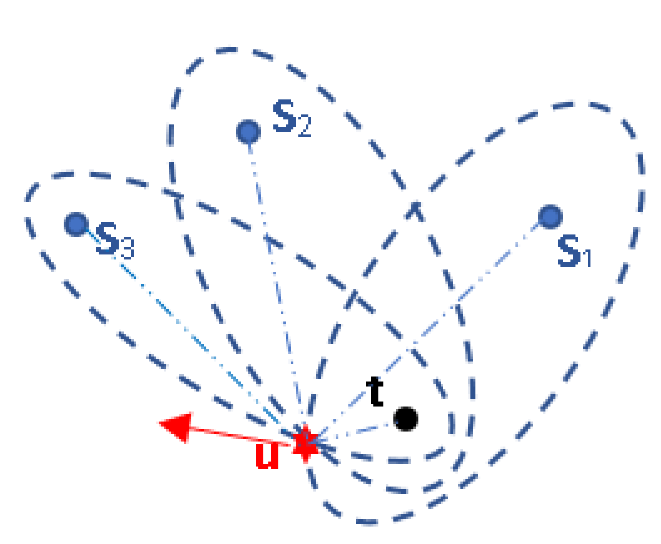
Figure 1 illustrates an elliptic scenario. The source reflects the emitted signal from a transmitter, and a receiver captures the reflected signal to locate the source after detection and classification processes [29]. For the 2-D case, the reflected signal’s propagation time defines an ellipse shape of possible source locations foci that represent the transmitter and receiver positions, as shown in the following figure. As the time delay elliptic measurement and distance are equivalent, we will use them interchangeably for our problem.

These measurements are taken and internally stored when the swarm of sensors fully captures the unknown system’s topology. The above elliptic technique can operate without synchronization requirement between the transmitter and the receiver [30,40].

The intersection of three or more ellipses yields the target location estimate. However, obtaining the intersection is not straightforward due to the highly nonlinear relationship between the measurements and the unknown target location [28,29,38]. When the frequency differences of the measurements are available, resulting from the relative motion between the source and receivers, we can improve the accuracy of the position estimate and identify the source velocity [38,39].

3. Proposed Node Localization Method

This method is an extension of the work [38] that employed the TDOA and FDOA measurements. In our sensor network application, we have applied time delay and frequency range (elliptic) techniques. The sensor network consists of M unknown sensors that need to be determined and N anchors that are placed at precisely known positions, where $N<<M$. The proposed method uses several assumptions: (i) at least three anchors/pseudo anchors do not lie on a straight line, (ii) at least three noncollinear anchors have a connection with the sensor that needs to be localized, (iii) the noises in the range of measurements are independent of each other, (iv) the standard deviation of the noise is marginal compared to the actual time delay and frequency range (elliptic) values for simplification purpose. We have followed the same steps in [38] starting from Equation (3) for the two-dimensional case. The true elliptic distances of Equation (3) can be written as

$$d_{it}^o=d_i^o+d_t^o,i=1,2,3,\dots ,N.$$

(4)

The transmitter $\mathbf{t}$ is assumed to be any node in the anchor group. Connectivity knowledge is important when grouping the anchors in the range of unknown sensors that need to be localized. Upon rewriting Equation (4) as $d_{it}^o-d_t^o=d_i^o$, squaring both sides, and substituting for ${d_i^o}^2$ and ${d_t^o}^2$, we arrive at a set of elliptic equations:

$${d_{it}^o}^2-2d_{it}^o{d_t}^o={\mathbf{s}}_i^T{\mathbf{s}}_i-{\mathbf{t}}^{\mathit{T}}\mathbf{t}-\mathbf{2}{({\mathbf{s}}_i-\mathbf{t})}^{\mathit{T}}\mathbf{u},i=1,2,3,\dots ,N.$$

(5)

The above elliptic equations alone allow computing the estimation of source position without the velocity, and they may not be sufficient to provide adequate accuracy to the position estimation [38,41]. Hence, the frequency range measurements are used to enhance the position estimate accuracy and evaluate the unknown sensor velocity.

The time derivative of $\left(d_i^o\right)$ expresses the relationship between sensor location parameters and the rate of the range [38]:

$${\acute{d}}_i^o=\frac{{(\acute{\mathbf{u}}-{\acute{\mathbf{s}}}_i)}^T(\mathbf{u}-{\mathbf{s}}_i)}{d_i^o}$$

(6)

Taking the time derivative of Equation (5) and rearranging it again, we arrive at a set of frequency range measurement equations:

$$2\left({\acute{d}}_{it}^o{d}_{it}^o-{{\acute{d}}_{it}^{o}d}_1^o-d_{it}^o{\acute{d}}_t^o\right)=2({\acute{{\mathbf{s}}_i}}^T{\mathbf{s}}_i-{\acute{\mathbf{t}}}^T\mathbf{t}-(\acute{\mathbf{t}}-{\acute{\mathbf{s}}}_i{)}^T\mathbf{u}-\left({\mathbf{t}-{\mathbf{s}}_i)}^{\mathbf{T}}\acute{\mathbf{u}}\right)$$

(7)

In the presence of elliptic range and frequency range noise, replacing the true range and range rate in Equations (5) and (7) by their noisy values and rearrangement, leads to an error vector equation:

$${\mathbf{\varrho }}_1={\mathit{z}}_1-{\mathbf{G}}_{\mathbf{1}}{\mathbf{\theta }}_1$$

(8)

where the vector ${\mathbf{\theta }}_1={[{\mathbf{u}}^{\mathbf{T}},d_t^o,{\acute{\mathbf{u}}}^T,{\acute{d}}_t^o]}^T$ contains the unknown source location parameters and two nuisance variables $d_t^o$ and ${\acute{d}}_t^o$, and

$${\mathit{z}}_1=\left[\begin{array}{c}{d}_{1t}^2-{\mathbf{s}}_1^T{\mathbf{s}}_1+{\mathbf{t}}^T\mathbf{t}\\ ⋮\\ d_{Nt}^2-{\mathbf{s}}_N^T{\mathbf{s}}_N+{\mathbf{t}}^T\mathbf{t}\\ {2(\acute{d}}_{1t}{d}_{1t}-{{\acute{\mathbf{s}}}_1^T\mathbf{s}}_1+{\acute{\mathbf{t}}}^T\mathbf{t})\\ ⋮\\ 2({\acute{d}}_{Nt}{d}_{Nt}-{{\acute{\mathbf{s}}}_N^T\mathbf{s}}_N+{\acute{\mathbf{t}}}^T\mathbf{t})\end{array}\right]and{\mathbf{G}}_{\mathbf{1}}=\mathbf{2}\left[\begin{array}{cccc}{(\mathbf{t}-{\mathbf{s}}_1)}^T& d_{1t}& {\mathbf{0}}^T& 0\\ ⋮& ⋮& ⋮& ⋮\\ {(\mathbf{t}-{\mathbf{s}}_N)}^T& d_{Nt}& {\mathbf{0}}^T& 0\\ (\acute{\mathbf{t}}-{{\acute{\mathbf{s}}}_1)}^T& {\acute{d}}_{1t}& (\mathbf{t}-{{\mathbf{s}}_1)}^T& d_{1t}\\ ⋮& ⋮& ⋮& ⋮\\ (\acute{\mathbf{t}}-{{\acute{\mathbf{s}}}_N)}^T& {\acute{d}}_{Nt}& {(\mathbf{t}-{\mathbf{s}}_N)}^T& d_{Nt}\end{array}\right]$$

(9)

where $\mathbf{0}$ is a $(2\ast 1)$ zero vector. Notice that second-order error terms have been disregarded. Hence, in the first stage processing, the weighted LS solution of ${\mathbf{\theta }}_1$ is

$${\mathbf{\theta }}_1={\left({\mathbf{G}}_{\mathbf{1}}^T{\mathbf{W}}_{\mathbf{1}}{\mathbf{G}}_{\mathbf{1}}\right)}^{-1}{{\mathbf{G}}_{\mathbf{1}}}^T{\mathbf{W}}_{\mathbf{1}}{\mathit{z}}_{\mathbf{1}}$$

(10)

and

$$Cov\left({\mathbf{\theta }}_1\right)={\left({\mathbf{G}}_{\mathbf{1}}^T{\mathbf{W}}_{\mathbf{1}}{\mathbf{G}}_{\mathbf{1}}\right)}^{-1}$$

(11)

where ${\mathbf{W}}_{\mathbf{1}}=E{\left[{{\mathbf{\varrho }}_{\mathbf{1}}{\mathbf{\varrho }}_{\mathbf{1}}}^T\right]}^{-1}$ expresses a positive definite weighting matrix. According to the assumption (iv), the ${\mathbf{\varrho }}_{\mathbf{1}}$ is zero mean asymptotically at ${\mathit{\theta }}_1^o$. Hence, ${\mathit{\theta }}_1$ is asymptotically unbiased. Next, we use Equations (10) and (11) to enhance the accuracy of the sensor node position estimate $\mathbf{u}$.

From the first stage of WLS, we have $\tilde{\mathbf{u}}={\mathbf{\theta }}_1(1:2)$ is an estimator of $\mathbf{u}$ and $\widetilde{\acute{\mathbf{u}}}={\mathbf{\theta }}_1(4:5)$ is an estimator of $\acute{\mathbf{u}}$. To this end, we construct another set of equations after applying the second stage of WLS and rearranging them by some simplification yields:

$${\mathbf{\varrho }}_2={\mathit{z}}_2-{\mathbf{G}}_{\mathbf{2}}{\mathbf{\theta }}_2$$

(12)

where

$${\mathbf{\varrho }}_2{|}_{{\mathbf{\theta }}_2={\mathbf{\theta }}_2^o}=\Delta {\mathit{z}}_2\approx {\mathbf{B}}_2\Delta {\mathbf{\theta }}_1$$

(13)

and

$$\begin{array}{c}{\mathit{z}}_{\mathbf{2}}=\left[\begin{array}{c}\begin{array}{c}\begin{array}{c}({\mathbf{\theta }}_{1,u}-\mathbf{t})⨀({\mathbf{\theta }}_{1,u}-\mathbf{t})\\ {{\mathit{\theta }}_1}^2\left(3\right)\end{array}\\ ({\mathbf{\theta }}_{1,\acute{u}}-\acute{\mathbf{t}})⨀({\mathbf{\theta }}_{1,u}-\mathbf{t})\end{array}\\ {\mathit{\theta }}_1\left(3\right){\mathit{\theta }}_1\left(6\right)\end{array}\right],{\mathbf{B}}_{\mathbf{2}}=\left[\begin{array}{cccc}2diag\left\{\mathbf{u}-\mathbf{t}\right\}& \mathbf{0}& \mathbf{O}& \mathbf{0}\\ {\mathbf{0}}^T& 2d_t^o& {\mathbf{0}}^T& 0\\ diag\left\{\acute{\mathbf{u}}-\acute{\mathbf{t}}\right\}& \mathbf{0}& diag\left\{\mathbf{u}-\mathbf{t}\right\}& \mathbf{0}\\ {\mathbf{0}}^T& {\acute{d}}_t^o& {\mathbf{0}}^T& d_t^o\end{array}\right],\\ {\mathbf{G}}_{\mathbf{2}}=\left[\begin{array}{cc}\begin{array}{c}{\mathbf{I}}_{\mathbf{2}}\\ {\mathbf{1}}^T\end{array}& \begin{array}{c}\mathbf{O}\\ {\mathbf{0}}^T\end{array}\\ \begin{array}{c}\mathbf{0}\\ {\mathbf{0}}^T\end{array}& \begin{array}{c}{\mathbf{I}}_{\mathbf{2}}\\ {\mathbf{1}}^T\end{array}\end{array}\right],{\mathbf{\theta }}_2=\left[\begin{array}{c}(\mathbf{u}-\mathbf{t})⨀(\mathbf{u}-\mathbf{t})\\ (\acute{\mathbf{u}}-{\acute{\mathbf{t}}}_{\mathbf{1}})⨀(\mathbf{u}-\mathbf{t})\end{array}\right]\end{array}$$

(14)

where $⨀$ is the Hadamard product operator, $\mathbf{0}\&\mathbf{1}$ are zero and unity vectors of $(2\ast 1)$, respectively, and ${\mathbf{I}}_{\mathbf{2}}\&\mathbf{O}$ are identity and zero matrices of $(2\ast 2)$, respectively. Applying WLS again to minimize the weight of the second norm of ${\mathbf{\varrho }}_2$, with a positive definite matrix ${\mathbf{W}}_{\mathbf{2}}$, produces

$${\mathbf{\theta }}_2={\left({\mathbf{G}}_{\mathbf{2}}^T{\mathbf{W}}_{\mathbf{2}}{\mathbf{G}}_{\mathbf{2}}\right)}^{-1}{\mathbf{G}}_{\mathbf{2}}^T{\mathbf{W}}_{\mathbf{2}}{\mathit{z}}_{\mathbf{2}}$$

(15)

The ${\mathbf{W}}_{\mathbf{2}}$ that attains the minimum parameter variance of ${\mathbf{\theta }}_2$ is $E{\left[{{\mathbf{\varrho }}_{\mathbf{2}}{\mathbf{\varrho }}_{\mathbf{2}}}^T{|}_{{\mathbf{\theta }}_2^o}\right]}^{-1}$ [42]. After ignoring the second-order error terms, multiplying Equation (13) with its transpose, taking the expectation value and inverting it, gives the weighting matrix ${\mathbf{W}}_{\mathbf{2}}$.

$${\mathbf{W}}_{\mathbf{2}}={\mathbf{B}}_{\mathbf{2}}^{-T}{Cov(\mathbf{\theta }}_1{)}^{-\mathbf{1}}{\mathbf{B}}_{\mathbf{2}}^{-\mathbf{1}}$$

(16)

We have ${\mathbf{\theta }}_2^o={\left({\mathbf{G}}_{\mathbf{2}}^T{\mathbf{W}}_{\mathbf{2}}{\mathbf{G}}_{\mathbf{2}}\right)}^{-1}{\mathbf{G}}_{\mathbf{2}}^T{\mathbf{W}}_{\mathbf{2}}{{z}}_{\mathbf{2}}^o={\left({\mathbf{G}}_{\mathbf{2}}^T{\mathbf{W}}_{\mathbf{2}}{\mathbf{G}}_{\mathbf{2}}\right)}^{-1}{\mathbf{G}}_{\mathbf{2}}^T{\mathbf{W}}_{\mathbf{2}}{\mathbf{\theta }}_2^o$. Hence, subtracting both sides of Equation (15) by ${\mathbf{\theta }}_2^o$ gives

$$\Delta {\mathbf{\theta }}_2={\left({\mathbf{G}}_{\mathbf{2}}^T{\mathbf{W}}_{\mathbf{2}}{\mathbf{G}}_{\mathbf{2}}\right)}^{-1}{\mathbf{G}}_{\mathbf{2}}^T{\mathbf{W}}_{\mathbf{2}}\Delta {\mathit{z}}_{\mathbf{2}}$$

(17)

From Equation (13), ${\mathbf{W}}_{\mathbf{2}}^{-1}=E[\Delta {{\mathit{z}}_{\mathbf{2}}\Delta {\mathit{z}}_{\mathbf{2}}}^T]$ and applying the assumption (iv) in Section 3 makes the G2 matrix constant. Hence, post-multiplying Equation (17) by its transpose and taking expectation gives the covariance matrix of ${\mathbf{\theta }}_2$ as shown in the following equation:

$$Cov\left({\mathbf{\theta }}_2\right)={\left({\mathbf{G}}_{\mathbf{2}}^T{\mathbf{W}}_{\mathbf{2}}{\mathbf{G}}_{\mathbf{2}}\right)}^{-1}.$$

(18)

From the definition of ${\mathbf{\theta }}_2$ in Equation (14), the final source position and velocity estimate of $\mathbf{u}$ after the refinement process is

$$\widehat{\mathbf{u}}=\Lambda \left[{\left({\mathit{\theta }}_2\left(1\right)\right)}^{0.5};{\left({\mathit{\theta }}_2\left(2\right)\right)}^{0.5}\right]+\mathbf{t}and\widehat{\acute{\mathbf{u}}}=\Lambda \left[\frac{{\mathit{\theta }}_2\left(3\right)}{{\left({\mathit{\theta }}_2\left(1\right)\right)}^{0.5}};\frac{{\mathit{\theta }}_2\left(4\right)}{{\left({\mathit{\theta }}_2\left(2\right)\right)}^{0.5}}\right]+\acute{\mathbf{t}}$$

(19)

where $\Lambda =diag\left\{sgn\left({\mathbf{\theta }}_{1,\mathbf{u}}-\mathbf{t}\right)\right\}$ with the aim of removing the sign ambiguity from the square root operation. It is worth mentioning that: (i) the above elliptic technique can operate without synchronization requirement between the transmitter and receiver [30,40], (ii) using different reference transmitters neither affects the information quality from the measurements nor affects the location precision since the weighting matrices ${\mathbf{W}}_{\mathbf{1}}$ and ${\mathbf{W}}_{\mathbf{2}}$ in Equations (11) and (16) are introduced. (iii) since the near-field scenario is applied, then, the proposed algorithm may need one or two iterations to give an accurate solution that reaches the CRLB under Gaussian noise [38]. (iv) The elliptic-based localization problem is challenging because the source location parameters and the sensor positions are nonlinearly related to the elliptic measurements. Therefore, the proposed closed-form solution is developed to handle the nonlinearity in the elliptic equation. (v) The thresholding effect can happen due to the nonlinear nature of the problem when the variance of the node position error increases [42]. This thresholding phenomenon in the proposed method is due to ignoring the second-order error terms in deriving the solution, which is not valid when the noise is significant.

4. Sequential Localization Framework

Challenging real-world sensor network sequential-localization configurations are considered here, in which the network comprises a large number of unknown wireless sensor nodes and has only several anchors. Our task is to explore and identify some unreachable system properties, which can be performed by determining the underlying sensor localization.

The developed single-node closed-form solution is suitable to resolve the obstacle of unknown remote systems in the WSN since it does not need an initial guess solution, and it is computationally less complex.

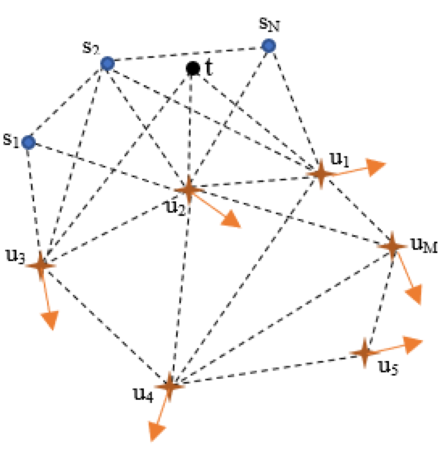
Figure 2 describes the anchor-based sensors network that considers two positioning parameters: time delay and range frequency elliptic techniques, where anchors, unknown sensors, and the transmitter are represented by solid blue circles, brown stars, and solid black circle, respectively. This network is rated as a partially connected network. The line connected in the plot is used to interpret the existence of specific measurements. In the figure, the unknown nodes at ${\mathbf{u}}_{\mathbf{4}}$, ${\mathbf{u}}_{\mathbf{5}}$, and others are invisible as they are not in the communication range of the reference nodes. Hence, it is considered a second tier in the offline localization process. This scenario is more realistic for a large-scale sensor network where some anchors can only communicate with a few neighboring sensor nodes. Thus, the connectivity information can also be exploited to cluster anchors and unknown sensors for the localization process.

In the first tier, which is similar to a fully connected network case, the unknown nodes (${\mathbf{u}}_{\mathbf{1}},{\mathbf{u}}_{\mathbf{2}},{\mathbf{u}}_{\mathbf{3}}$) within the communication range of the anchors are localized first. While in the second tier, and according to the connectivity, the unknown nodes with estimated positions and velocities are considered pseudo anchors to determine the following unknown sensor positions under some uncertainty of position and velocity. The uncertainty is eliminated by applying the refinement process of the second WLS minimization. This procedure is repeated for the next cluster until all the unknown sensors in the network are localized successfully. We emphasize that the number of N omits the transmitter node. 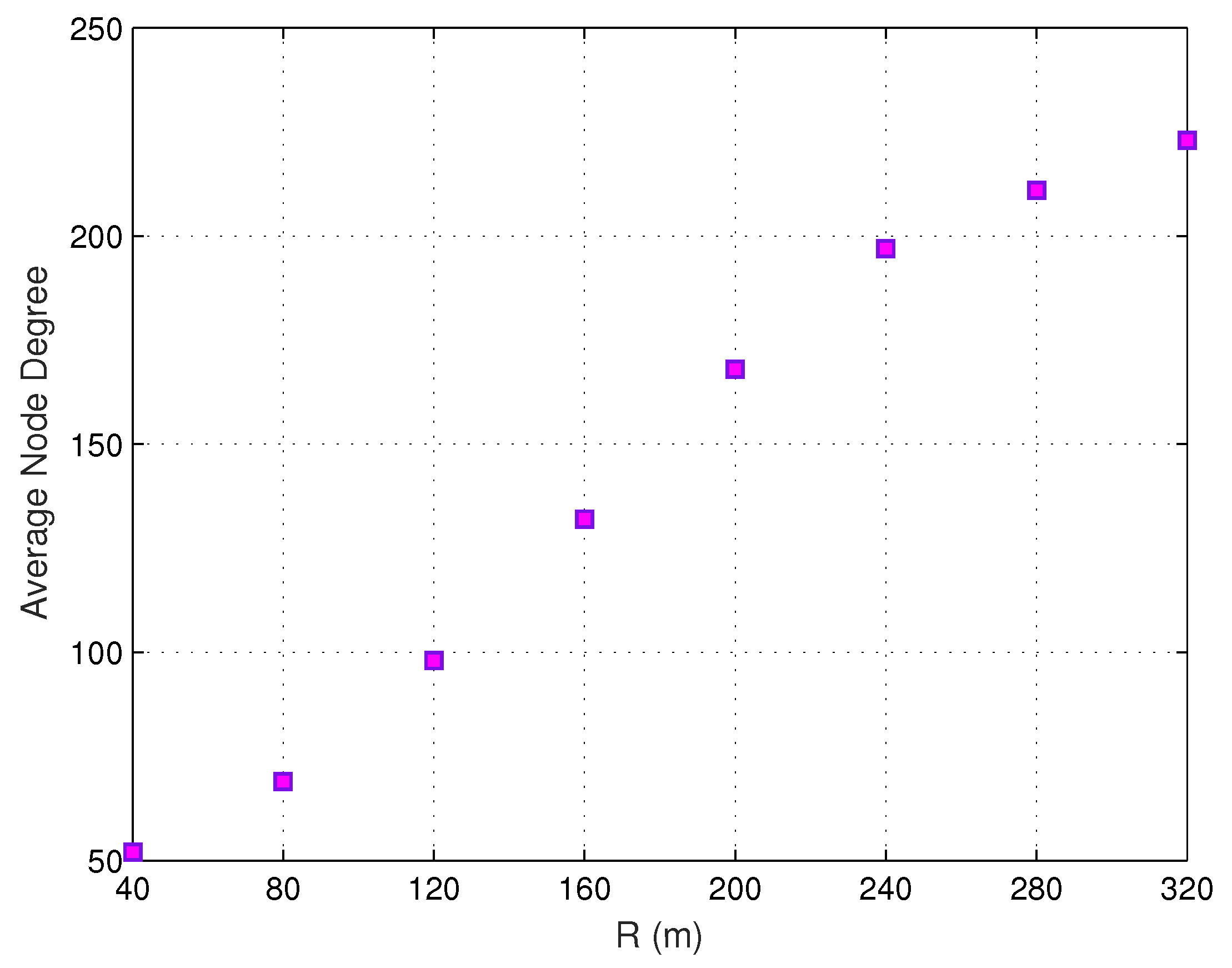Due to the sequential framework process, the number of N may vary according to the number of pseudo anchors in each cluster. In this context, increasing the number of anchors can improve the localization accuracy by raising the average node degree. More accurate position estimates will be obtained when the network has a large average node degree [43].

5. Performance Evaluation

Challenging real-world sensor network sequential-localization configurations are considered here. First the sensor nodes are deployed randomly inside the system, which is assumed to have one inflow and outflow, with the knowledge of connectivity of the entire network. Then, after the nodes fully occupy the system, the offline localization process can be performed at a particular timestamp.

5.1. Comparison with the CRLB

Our reliable benchmark reference for evaluating the proposed estimator is the Cramér–Rao lower bound (CRLB) [42]. We have followed [38], with slight differences, to derive the CRLB using the time delay elliptic and frequency range measurements. The CRLB for the underlying problem can be defined as

$$\mathrm{CRLB}={\left\{\left({\left(\frac{\partial {\mathit{q}}^o\left(\mathit{\phi }\right)}{\partial \mathit{\phi }}\right)}^T{\mathit{Q}}^{-1}\left(\frac{\partial {\mathit{q}}^o\left(\mathit{\phi }\right)}{\partial \mathit{\phi }}\right)\right){|}_{\mathit{\phi }={\mathit{\phi }}^o}\right\}}^{-1}$$

(20)

where ${\mathit{\phi }}^o$ = ${\left[\mathbf{u},\acute{\mathbf{u}}\right]}^T$, ${\mathit{q}}^o={\left[d_{1t}^o,d_{2t}^o,\dots ,r_{Nt}^o,{\acute{d}}_{1t}^o,{\acute{d}}_{2t}^o,\dots ,{\acute{d}}_{Nt}^o\right]}^T={\left[{\mathit{d}}^{oT},{\acute{\mathit{d}}}^{oT}\right]}^T$.

${\mathit{Q}}^{-1}$ is the inverse of the generating covariance of measurement error in our simulation and,

$$\frac{\partial {\mathit{q}}^o\left(\mathit{\phi }\right)}{\partial \mathit{\phi }}=\left[\begin{array}{cc}\frac{\partial {\mathit{d}}^o\left(\mathit{\phi }\right)}{\partial \mathbf{u}}& \frac{\partial {\mathit{d}}^o\left(\mathit{\phi }\right)}{\partial \acute{\mathbf{u}}}\\ \frac{\partial {\acute{\mathit{d}}}^o\left(\mathit{\phi }\right)}{\partial \mathbf{u}}& \frac{\partial {\acute{\mathit{d}}}^o\left(\mathit{\phi }\right)}{\partial \acute{\mathbf{u}}}\end{array}\right]$$

(21)

where

$$\frac{\partial {\mathit{d}}^o\left(\mathit{\phi }\right)}{\partial \mathbf{u}}=\frac{\partial {\acute{\mathit{d}}}^o\left(\mathit{\phi }\right)}{\partial \acute{\mathbf{u}}}=\frac{{(\mathbf{u}-{\mathbf{s}}_i)}^T}{d_i^o}+\frac{{(\mathbf{u}-\mathbf{t})}^T}{d_t^o}=\frac{\partial {\acute{\mathit{d}}}^o\left(\mathit{\phi }\right)}{\partial \acute{\mathbf{u}}},\frac{\partial {\mathit{d}}^o\left(\mathit{\phi }\right)}{\partial \acute{\mathbf{u}}}={\mathit{O}}_{(N\ast 2)}.$$

$$\frac{\partial {\acute{\mathit{d}}}^o\left(\mathit{\phi }\right)}{\partial \mathbf{u}}=\frac{{(\acute{\mathbf{u}}-{\acute{\mathbf{s}}}_i)}^T}{d_i^o}-\frac{{(\mathbf{u}-{\mathbf{s}}_i)}^T{\acute{d}}_i^o}{{d_i^o}^2}+\frac{{\left(\acute{\mathbf{u}}-\acute{\mathbf{t}}\right)}^T}{d_t^o}-\frac{{(\mathbf{u}-\mathbf{t})}^T{\acute{d}}_t^o}{{d_t^o}^2}.$$

5.2. Simulation

Simulated experiments have been performed for the 2-D case to assess the performance of the proposed approach under various amounts of measurement errors. We have assumed the standard noise deviation is slight relative to the actual time delay (elliptic) and frequency range values. Moreover, the second-stage processing substantially reduces the position and velocity standard deviations in this simulation experiment, reducing the position estimate bias and confirming that the proposed estimator is asymptotically unbiased. Hence, we neglected the bias in our study. The parameters are set as the following: (i) all unknown nodes are identical, have the same communication range R, and their antennas are isotropic. (ii) Availability of information about at least three anchor sensors for the 2-D case placed randomly at the insertion point of the unknown system. (iii) All sensors are neither lying on a straight line nor exchanging data with others. (iv) The (time delay) elliptic and frequency range noises are zero-mean Gaussian, and their covariance matrices are $\left({\sigma }_d^2\right)\mathbf{\rho }$ and $0.1\left({\sigma }_d^2\right)\mathbf{\rho }$, where $\mathbf{\rho }$ is equal to unity in the diagonal elements and 0 otherwise [28,29]. Thus, both the time delay elliptic and frequency range measurement noises were uncorrelated. This choice of the measurement errors’ covariance matrix (Q) corresponds to the MLE estimation of elliptic and frequency ranges [41] for equal and uncorrelated receiver noises. (v) For further accuracy refinement, iterative MLE via Taylor series (TS) linearization [42] has also been implemented using the same framework of the proposed method. Repeating the MLE solution calculation two times is enough to give an accurate estimation that reaches the CRLB under Gaussian noise. All nodes whose locations were successfully estimated may have a more accurate position estimate in which they act as initialization for the MLE implementation. The average of the Root Mean Square Error (RMSE) of the estimated positions is computed to examine the performance of each algorithm. In general, the average RMSE is defined using Equation (22).

$$\mathrm{RMSE}=\sqrt{\frac{1}{L\ast M}\left({\displaystyle {\displaystyle \sum }_1^L}{\displaystyle {\displaystyle \sum }_{j=1}^M}\Vert [{\widehat{\mathbf{u}}}_j-{\mathbf{u}}_j{\Vert }_2^2\right)}$$

(22)

where the number of ensemble runs L is 1000.

Two configurations have been implemented in this part. Figure 3 and Figure 4 present the accuracy and the topology of the first configuration. This scenario consists of 8 anchors (inside a black rectangle) placed at the input and output points and 300 unknown sensor nodes deployed in the unknown system assumed to have a U shape. Figure 3 displays the comparison among the proposed closed-form method (CFM), the estimated solution after passing the MLE implementation (MLE), and CRLB accuracy at the two different communication ranges $(R=40\&R=100)$. The plots show that CFM and MLE methods can reach CRLB accuracy.

Due to the high nonlinearity, sequential framework process, and thresholding behavior effect, both methods have deviated from the CRLB. Beyond noise level 1, the proposed CFM method deviates from the bound, whereas the MLE method has the best outcome. However, the refinement MLE approach deviates from the CRLB accuracy later.

The developed approach can work effectively with a $100\%$ LOS scenario. Having no (or few) obstacles increases the communication signal range. Without the presence of obstacles, the number of the known sensors (pseudo anchors) with an adequate communication strength will increase. As a result, the increase in the average node degree is used to estimate the position of the unknown sensor node with more accuracy.

Figure 4 and Figure 5 illustrate the topology of the distribution of the unknown sensors and their true and estimated positions using both methods at $R=40$ under noise power ${\sigma }^2=1$. The figures reveal a successful and effective WSN accommodation in exploring the unknown system.

The localization performance of the second configuration is demonstrated in Figure 6 and Figure 7. The configuration includes 100 unknown sensor nodes and 5 fixed nodes placed at the insertion point, as shown in Figure 7. In addition, the figure indicates that the proposed CFM method can detect the position of the unknown sensors with an accuracy reaching the CRLB for a wide range of noise levels. The results affirm that the proposed method with MLE refinement matches the real observations by reaching the CRLB accuracy with a better resistance for the thresholding effect than the CFM method.

A study of the relation between the average node degree and different values of communication range R for the first scheme is presented in Figure 8. The figure displays the positive correlation between the two variables: the communication range and the node degree. Increasing R leads to an increase in the number of anchors and receivers, improving the localization accuracy by raising the average node degree. As a result, more accurate position estimates will be obtained when the network has a considerable average node degree. However, since the estimation performance depends on the nature of the nonlinear problem, more accurate position estimates might not be obtainable due to the large node degree.

Based on the power consumption model (2), the required transmitter power for successful telecommunication between two network nodes is directly proportional to the distance between the nodes to the power n ($\propto d^n$), where $5\ge n>2$ for obstructed conditions of the system.

Utilizing the sequential localization approach can reduce the maximum line-of-sight distance required for successful localization. For the studied simulation scenarios, the maximum communication range required for successful sequential localization is $R=40$ and $R=15$ meters for noise level 1, as shown in Figure 4 and Figure 7; while the full range of the network ($d_{max}$), defined as the maximum distance between the farthest node and the anchors, is 410 and 125 meters, respectively. Altogether, the transmission power for successful communication between two successive sensors can be reduced by a factor equal to $\left(1-{\left(\frac{R}{d_{max}}\right)}^n\right)$. Thus, the theoretical reduction in the transmission power rate will be more than $98\%$ for the studied scenarios when $n>2$.

6. Conclusions

This paper presents a sequential sensor localization technique for the challenging application of exploring unknown bounded systems using mobile sensors equipped with limited transmission rates. A closed-form solution is devised and implemented for underground monitoring and remote sensing applications. The proposed approach yields the CRLB accuracy and successfully captures the unknown environment fully covered by an enormous number of sensor nodes. Furthermore, the developed localization algorithm can reduce the transmission power by more than 98% for the tested network scenarios when compare to the full range network localization approach. Thus, the developed localization approach can be exploited to design a smaller power module that reduces the cost of the sensing devices while sustaining a longer durability for efficient remote sensing and mapping observations. Future work will consist of designing and experimentally investigating a prototype of a wireless sensor device to explore an unbounded geometrical system using a low-range telecommunication signal transmission system.