Theoretical Computational Model for Cylindrical Permanent Magnet Coupling

Abstract

Permanent magnet coupling is extensively studied owing to its economic efficiency and stability. In this study, a computational model for cylindrical permanent magnet coupling (CPMC) was designed using the magnetic field division method to divide an air gap magnetic field. An equivalent magnetic circuit model was also designed based on the equivalent magnetic circuit method. The novelty of this study is that both the skin effect and the working point of the permanent magnet are taken into consideration to obtain the magnetic circuit and induce eddy current characteristics of permanent magnet coupling. Furthermore, a computational model was obtained for the transmission torque of the CPMC based on the principles of Faraday’s and Ampere’s laws. Additionally, the accuracy of the model was verified using a finite element simulation model and a test bench.

1. Introduction

Permanent magnet coupling is based on magnetic fields. It utilizes the non-contact relative motion between a permanent magnet and a conductor to induce an eddy current that, in turn, generates an induced magnetic field. The induced magnetic field then interacts with the original magnetic field and generates a torque, thereby realizing torque transmission between a motor and a load. Compared to fluid, rigid, or flexible couplings and other traditional transmission devices, permanent magnet coupling has many advantages, such as high reliability and stability, good vibration isolation, and easy maintenance. Therefore, permanent magnet coupling is extensively used in mining machinery and in the chemical, pharmaceutical, manufacturing, and other industrial fields.

To date, studies involving electromagnetic torque transmission devices have predominantly employed numerical analyses or analytical models. The finite element method (FEM) [1,2,3,4] accurately describes the electric and magnetic field distributions inside devices. However, it is time-consuming and highly resource-intensive. An analytical model is less accurate than the FEM, but the associated calculation is simple, and the model parameters can be easily modified; hence, it simplifies the device design, model selection, and maintenance processes.

Permanent magnet couplings are divided into two types based on the arrangement of the magnetic blocks. In the first type, the permanent magnet is embedded in a disk frame, and the main magnetic circuit direction is axial [5,6]. In the second type, the permanent magnet is embedded in a cylindrical frame, and the main magnetic circuit direction is radial; additionally, the conductor has a cylindrical structure [7,8,9]. Compared to the former, the latter can realize the complete separation of the conductor disk and permanent magnet disk. It can also disconnect from the motor when the load stalls, thus protecting the motor. In addition, the axial force of the former is expressed as the force along the radial direction of the cylindrical structure in the latter. The structural strength of each component is sufficient to meet the force requirements without the need to assemble any additional components. Previous studies on cylindrical permanent magnet coupling (CPMC) mostly employed the equivalent magnetic circuit method [10], combined Faraday’s and Ampere’s laws [11], established nonlinear models of cylindrical permanent magnet couplings, and investigated the impact of design parameters on the coupling performance [12,13].

Our research group has conducted research on disk permanent magnet coupling (DPMC). For example, Meng and Niu established a simulation model for DPMC and used Ansoft Maxwell to simulate and analyze the model’s torque and transient response [14]. Furthermore, Yuan et al. studied the overload protection characteristics of DPMC in a coal mine through a simulation analysis and experimental testing [15].

Cao et al. investigated the transient field, eddy current distribution, and temperature field of CPMC under the low-load condition (with a slip of 20 rpm) [16]. However, in engineering practice, CPMC generally operates under rated or high-load conditions rather than under low-load conditions. In addition, Cao et al.’s research results lack experimental verification. Therefore, a simulation study is required for the rated and high-load conditions, and the results must be verified experimentally.

The structure of a CPMC is shown in Figure 1. It is mainly composed of inner and outer steel drums, inner and outer permanent magnet blocks, inner and outer frames, and a conductor tube. In general, the conductor tube is the output side, which is connected to the output shaft, and the permanent magnet drum—which includes inner and outer permanent magnet drums—is the input side, which is connected to the input shaft. The permanent magnet block is a cuboid and is embedded in the frame; the magnetization direction of the permanent magnet is along the radial direction; the magnetization directions of the red and blue permanent magnet blocks are opposite; and there are air gaps between the conductor tube and the inner and outer frames, which can achieve non-contact transmission.

In previous studies, the actual working point of the permanent magnet was rarely considered. In the models proposed in the aforementioned studies, the magnetic flux density of the permanent magnet was related only to the remanence, which deviates from the actual working state of the permanent magnet. In addition, the skin effect on the uneven current distribution in the conductor was not considered. Furthermore, some mathematical models used relatively complex partial differential equations that are not conducive to practical engineering applications. From an experimental perspective, the rated powers of the motor and the permanent magnet coupling are approximately the same; thus, only the working characteristics of the permanent magnet coupling near the rated torque can be measured.

To address these gaps, we first used the magnetic field division method to properly divide the air gap magnetic field of the CPMC into different types of magnetic flux tubes. Then, we estimated the permeance values using the classic permeance calculation formula, in which the permanent magnet is equivalent to the series connection of the magnetomotive force (MMF) and magnetoresistance (MR). Next, we established an equivalent magnetic circuit model based on the actual magnetic flux tube arrangement using the equivalent magnetic circuit method. Subsequently, we determined the characteristics of the external magnetic circuit and magnitude of the induced MMF using Kirchhoff’s law for magnetic circuits. Further, we calculated the magnitude of the eddy current induced in the conductor tube using Faraday’s electromagnetic induction principle and calculated the Ampere force generated owing to the induced eddy current using Ampere’s law to obtain the torque transmission model of the CPMC. In addition, we established a finite element simulation model and simulated the distributions of the magnetic flux density, eddy current vector, and ohmic loss of the CPMC under the rated and high-load conditions; these simulations were then compared with those obtained under the low-load condition.

Finally, we verified the accuracy and working performance of the theoretical model via a test bench constructed using a high-power motor to test the extreme transmission torque of the coupling, and then the accuracy of the theoretical model was verified, and its working performance was also tested.

The rest of this paper is organized as follows: Section 2 established theoretical computational model of CPMC. In Section 3, we carried out simulation and experimental research, then did a comparison with other models. Section 4 summarizes the results of this study and directions for future research. Appendix A includes the list of acronyms (

Table A1. List of acronyms.

Acronym	Full Term
PMC	Permanent Magnet Coupling
CPMC	Cylinder Permanent Magnet Coupling
DPMC	Disk Permanent Magnet Coupling
FEA	Finite Element Analysis
FEM	Finite Element Analysis Method
MMF	Magnetomotive Force
MF	Magnetoresistance
3D	Three-Dimensional
AS-PMECC	Adjustable-Speed Permanent Magnet Eddy Current Coupling
RF-CPMC	Radial Flux Cylindrical Permanent Magnet Coupling
FC-CPMC	Flux-Concentrating Cylindrical Permanent Magnet Coupling

), notations and corresponding units used in this article (

Table A2. List of notations and corresponding units.

Notation	Full Term	Unit
B	Magnetic flux density	T
Br	Remanence	T
Bm	Magnetic flux density of permanent magnet working point	T
Bi	Magnetic flux density in magnetic flux tube i	T
H	Magnetic field intensity	A/m
Hm	Magnetic field intensity of permanent magnet working point	A/m
Φ	Magnetic flux	Wb
Φm	Main magnetic flux of magnetic circuit	Wb
Φi	Magnetic flux in magnetic flux tube i	Wb
Φa	Air gap magnetic flux	Wb
μ0	Vacuum permeability	H/m
μm	Relative permeability of permanent magnet	H/m
Λ	Permeance	H
Λi	Permeance of magnetic flux tube i	H
R	Magnetoresistance	H−1
Rm	Internal resistance of permanent magnet	H−1
Ri	Magnetoresistance of magnetic flux tube i	H−1
Am	Cross-sectional area of permanent magnet	m2
Ai	Cross-sectional area of flux tube i	m2
F	Magnetomotive force	A
Fad	Induced magnetic field magnetomotive force	A
ds	Skin depth	m
Δ	Skin effect coefficient	-
ω	Slip speed	rpm
n	Rotational speed	rpm
T	Torque	N.m
P	Power	kW

).

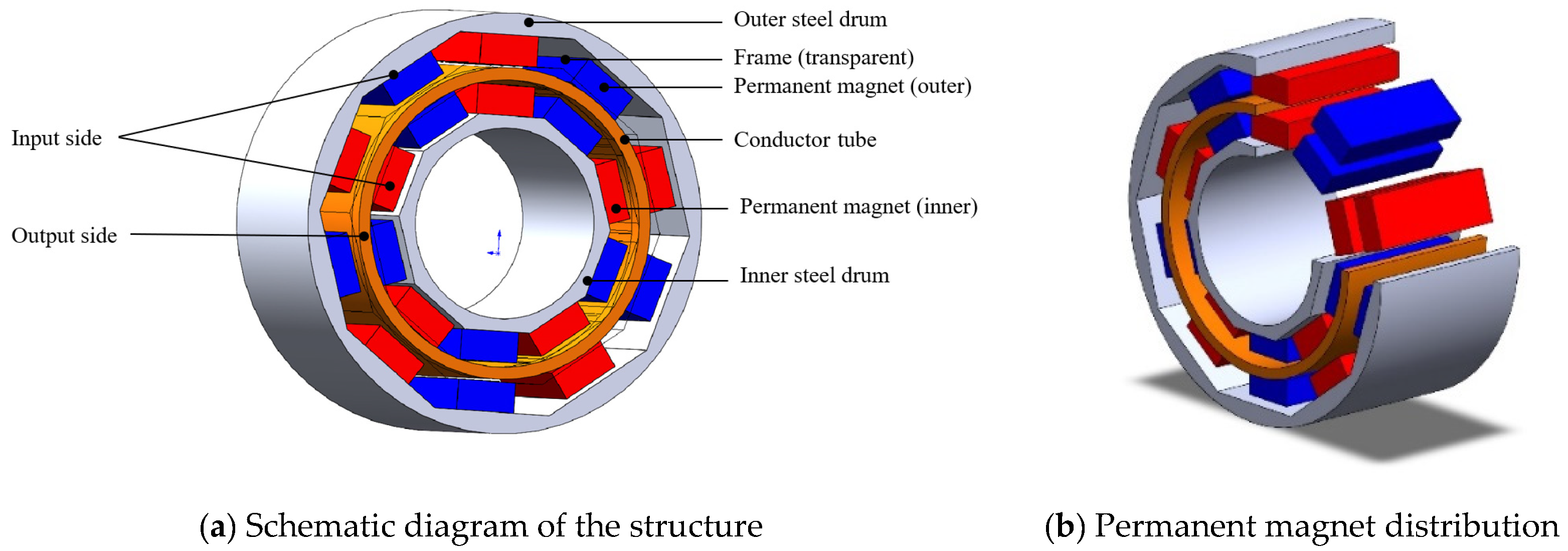
2. Theoretical Model

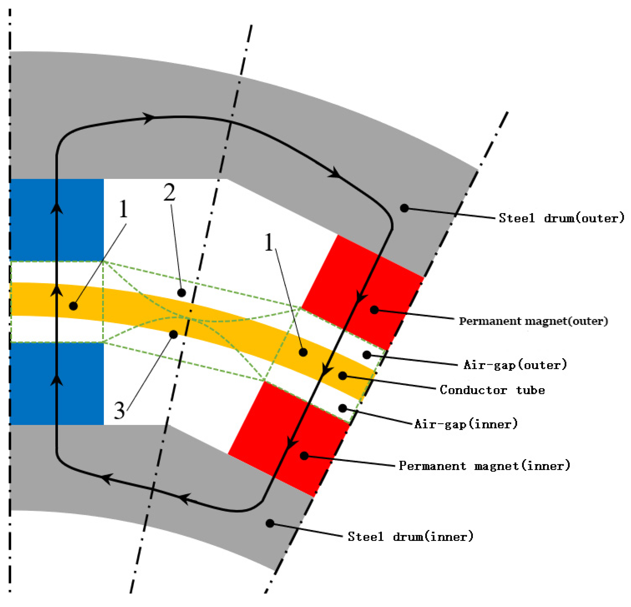
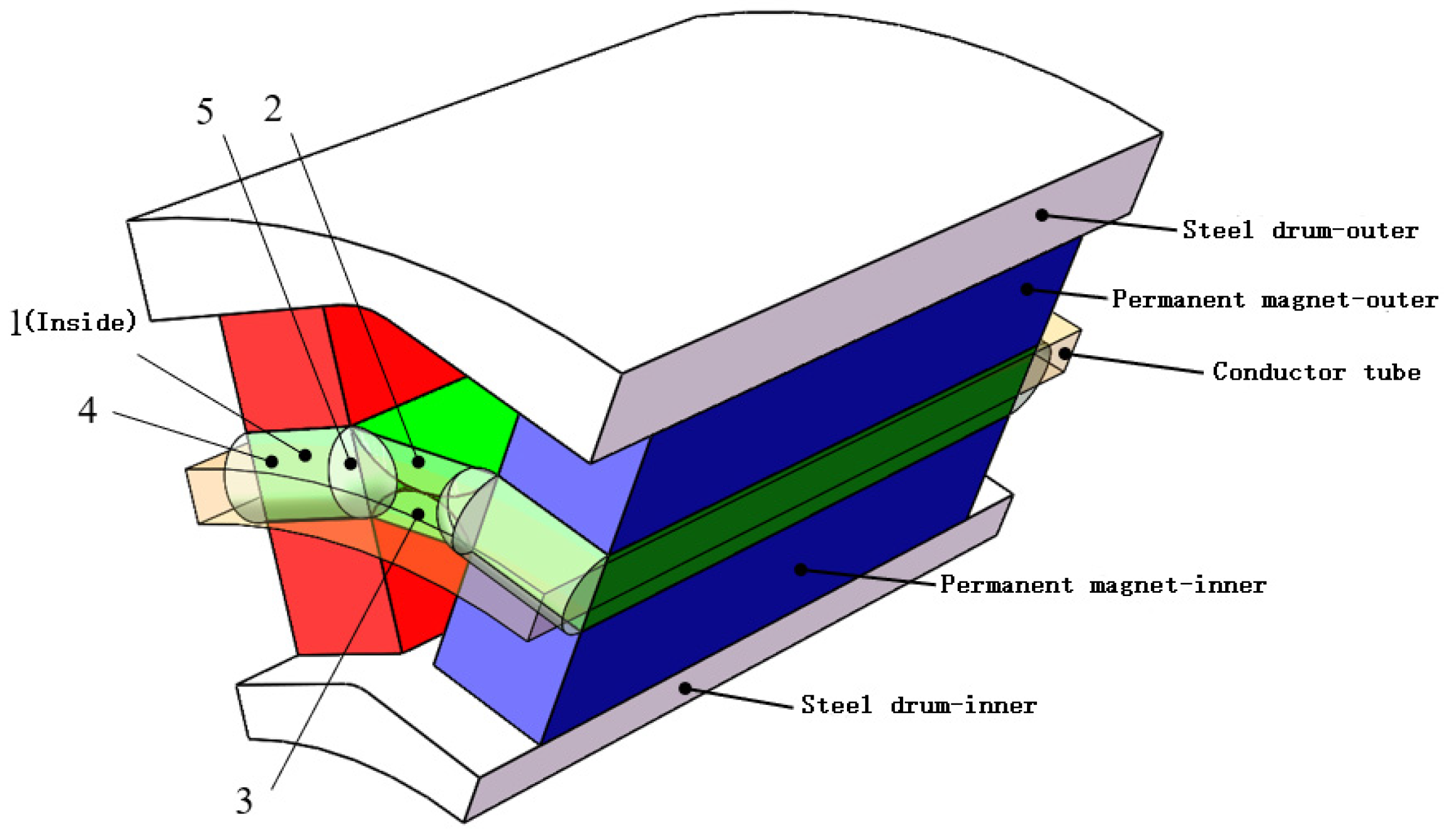
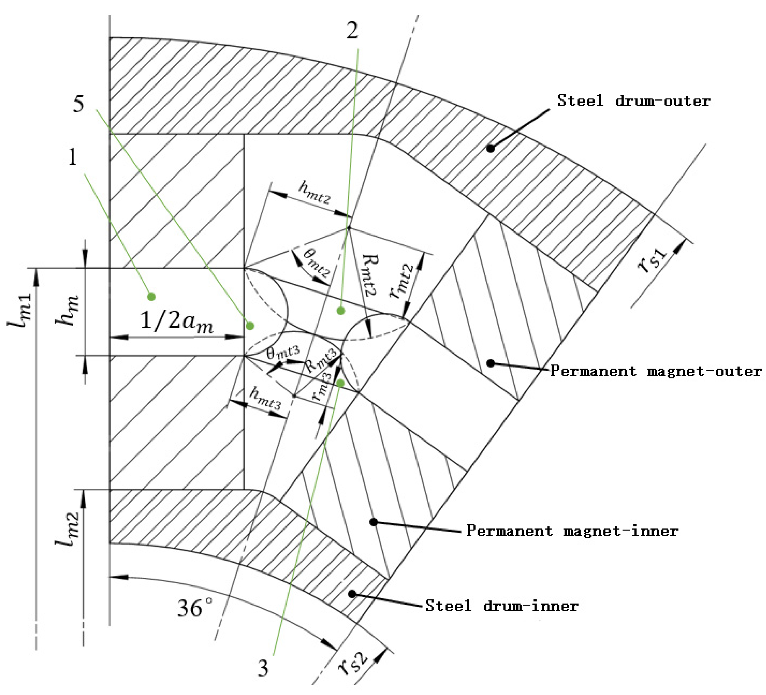
2.1. Magnetic Field Division

CPMC is symmetrical in the circumferential direction; hence, the objective of this study was to design a model for a single magnetic circuit. As shown in Figure 2, the main magnetic circuit and air gap magnetic flux leakage are divided into regular magnetic flux tubes using the magnetic field division method [17,18,19,20,21]. The permanent magnet is divided into two equal parts along the radial direction, and the polarization is in the radial direction; however, the direction of magnetization of the adjacently placed permanent magnets is opposite. The arrow in Figure 2 indicates the direction of the main magnetic circuit. First, it passes from the inner permanent magnet through the conductor tube and air gap to the outer permanent magnet (magnetic flux tube 1 enclosed by the green dashed lines). Then, it flows along the steel drum to the adjacent outer permanent magnet with the opposite polarization direction and again passes through the conductor tube and inner permanent magnet. Finally, it flows back to the inner permanent magnet through the inner steel drum. The air gap magnetic flux leakage is attributed to magnetic flux tubes 2 and 3 enclosed by the green dashed lines, which are two semi-arc magnetic flux tubes connected in series.

The distribution of all the magnetic flux tubes is shown in Figure 3. The yellow transparent area represents the conductor disk, and the green area represents the different magnetic flux tubes. The magnetic field between the inner and outer permanent magnets includes the cuboid magnetic flux tube 1, 1/2 cylindrical magnetic flux tube 4 at the axial ends, and 1/4 spherical magnetic flux tube 5.

The characteristic dimensions of each magnetic flux tube are drawn according to the actual structure of the CPMC, as shown in Figure 4.

The regular magnetic flux tube 1 is a cuboid, and its permeance is the ratio of the average cross-sectional area of the magnetic flux tube to the average length of the magnetic lines of force inside the magnetic flux tube, as given in Equation (1):

$${\Lambda }_1=\frac{{\mu }_0{a}_m{b}_m}{2l_g},$$

(1)

where ${\Lambda }_i$ is the permeance (i is the numbering of the magnetic flux tube, in this case i = 1), and $R_i$ is the MR of the magnetic flux tube; ${\Lambda }_i$ and $R_i$ are reciprocals of each other.

According to the permeance calculation formula of a typical semi-arc magnetic flux tube, the permeance values of magnetic flux tubes 2 and 3 are given in Equations (2) and (3) as

$${\Lambda }_2=\frac{1.335{\mu }_0{b}_m\left(R_{mt2}-r_{mt2}\right)}{2\left(h_{mt2}+{\theta }_{mt2}{R}_{mt2}\right)}$$

(2)

$${\Lambda }_3=\frac{1.335{\mu }_0{b}_m\left(R_{mt3}-r_{mt3}\right)}{2\left(h_{mt3}+{\theta }_{mt3}{R}_{mt3}\right)}$$

(3)

The permeance of magnetic flux tube 4 is given by the permeance calculation formula of a typical 1/4 cylindrical magnetic flux tube as follows:

$${\Lambda }_4=0.26{\mu }_0{a}_m$$

(4)

In addition, the permeance of magnetic flux tube 5 is given by the permeance calculation formula of a typical 1/4 spherical magnetic flux tube as follows:

$${\Lambda }_5=0.077{\mu }_0{l}_g$$

(5)

2.2. Equivalent Magnetic Circuit Model

A permanent magnet is modeled to be equivalent to a series connection of the MMF and MR using the equivalent surface current method [22]. The MMF of the permanent magnet is defined as $F_c=H_m{h}_m$, where H_m is the magnetic field strength when the permanent magnet is working, and h_m is the length of the permanent magnet in the magnetization direction.

As shown in Figure 5, the MMF of the cuboid permanent magnet is equivalent to the sum of the currents flowing on the four lateral surfaces parallel to the magnetization direction. In addition, the current density of the current layer is numerically equal to the magnetic field intensity of the permanent magnet. MR is the internal resistance of the permanent magnet as defined by the following equation:

$$R_m=\frac{h_m}{{\mu }_0{\mu }_r{A}_m},$$

(6)

where ${\mu }_0$ and ${\mu }_r$ are the vacuum permeability and the relative permeability of the permanent magnet, respectively, and $A_m$ is the cross-sectional area of the permanent magnet in the magnetization direction.

When making the permanent magnet equivalent to the series connection of the MMF and MR using the equivalent surface current method, the working point of the permanent magnet needs to be considered [23,24]. This point is located on the recovery curve. For a permanent magnet made of neodymium iron boron, the recovery curve is approximately a straight line, which coincides with the demagnetization curve at room temperature. By multiplying the abscissa and ordinate of the recovery curve ($B=f\left(H\right)$) by the thickness along the magnetization direction and the cross-sectional area of the permanent magnet, the relationship curve between the permanent magnet flux and the MMF (${\Phi }_m=f\left(F_m\right)$) can be obtained, as shown in Figure 6, where the characteristic curve of the permanent magnet outside the magnetic circuit is ${\Phi }_{\delta }=f\left(F\right)$. When the permanent magnet coupling is stable, a slip speed exists between the permanent magnet and the conductor, resulting in an eddy current being induced in the conductor tube. The induced magnetic field generated by the induced eddy current imposes a reaction force on the original magnetic field. In Figure 6, the generated induced electromotive force is $F_{ad}$. Therefore, when calculating the permanent magnet working point, the external characteristic curve should be shifted to the left by $F_{ad}$. Then, the intersection point of the external magnetic circuit characteristic curve and the demagnetization curve will be ($F_m,{\Phi }_m$); that is, the permanent magnet will provide an MMF of $F_m$ and a magnetic flux of ${\Phi }_m$ under this working condition.

In this study, a permanent magnet made of neodymium iron boron was used for permanent magnet coupling. The recovery curve is presented in Figure 6; the working point is on the recovery curve. Under normal working conditions, the recovery curve coincides with the demagnetization curve and can be approximated as a straight line that connects points ($-H_c$, 0) and (0,$B_r$). The magnetic flux density and magnetic field intensity of the permanent magnet working point are B_m1 and H_m1 for the outer permanent magnet and B_m2 and H_m2 for the inner permanent magnet. To obtain the relationship between the magnetic flux density and magnetic field intensity at the working point of the permanent magnet, the formula describing this relationship, that is,$B={\mu }_0{\mu }_{rm}H$, is combined with the recovery curve expression for the permanent magnet. This is represented as follows:

$${\mu }_0{\mu }_{rm}{H}_{m1}=B_r-B_{m1}$$

(7)

$${\mu }_0{\mu }_{rm}{H}_{m2}=B_r-B_{m2}$$

(8)

The main magnetic flux of the magnetic circuit is equal to the product of the magnetic flux density at the working point of the permanent magnet and its cross-sectional area; it is given by the following equations:

$${\Phi }_{m1}=A_m{B}_{m1}$$

(9)

$${\Phi }_{m2}=A_m{B}_{m2}$$

(10)

The magnetic flux of magnetic flux tube i is equal to

$${\Phi }_i=A_i{B}_i,$$

(11)

where A_i is the average cross-sectional area in the direction of the magnetic induction lines in the magnetic flux tube that can be calculated from the structural parameters of the CPMC, and B_i is the magnetic flux density in the magnetic flux tube. The relationship between the air gap magnetic flux ${\Phi }_a$ and the MR of each part is given in Equation (12):

$${\Phi }_a\left(\frac{2R_1{R}_4{R}_5}{2R_4{R}_5+R_1{R}_5+R_1{R}_4}\right)=R_1{\Phi }_1=R_4{\Phi }_5=R_5{\Phi }_5$$

(12)

By combining the magnetic field division method described in Section 2.1 with the structural relationship between the main and air gap magnetic circuits, an equivalent circuit model was established, and this model is presented in Figure 7.

In Figure 7, the magnetic flux through the outer and inner permanent magnets is represented as ${\Phi }_{m1}$ and ${\Phi }_{m2}$, respectively. The left air gap magnetic flux is composed of one magnetic flux tube 1, two magnetic flux tubes 4, and two magnetic flux tubes 5 in series; the magnetic flux is represented as ${\Phi }_a$. The magnetic fluxes of the air gap leakage for magnetic flux tubes 2 and 3 are ${\Phi }_2$ and ${\Phi }_3$, respectively. The MMFs of the induced magnetic fields for the outer and inner permanent magnets are $F_{c1}$ and $F_{c2}$, respectively. A single magnetic circuit divides the permanent magnet into two equal parts; therefore, the MR of the permanent magnet is $2R_m$. As the equivalent circuit is symmetrical, the MMFs of the induced magnetic fields on the left and right are both equal to $F_{ad}$. The directions of the magnetic flux and MMF depicted in Figure 7 are positive. The inner and outer steel drums are made of silicon steel with high permeability (the saturation permeability is approximately 4000 times that of air) and low conductivity (approximately 1/10 of the conductor tube). Thus, its MR is extremely small relative to the internal resistance of the permanent magnets and MR of the air gap. Hence, it can be ignored, that is, $R_{s1}=R_{s2}=0$.

According to the equivalent circuit diagram shown in Figure 7 and Kirchhoff’s law for magnetic circuits, the following set of equations can be derived from points A and B and loops 1 to 3.

$$\{\begin{array}{c}{\Phi }_a+{\Phi }_2-{\Phi }_{m1}=0\\ {\Phi }_a+{\Phi }_3-{\Phi }_{m2}=0\\ 4R_m{\Phi }_{m1}+R_2{\Phi }_2=2F_{c1}\\ \left(\frac{2R_1{R}_4{R}_5}{2R_4{R}_5+R_1{R}_5+R_1{R}_4}\right){\Phi }_a-R_2{\Phi }_2-R_3{\Phi }_3=-2F_{ad}\\ 4R_m{\Phi }_{m2}+R_3{\Phi }_3=2F_{c2}\end{array}$$

(13)

Equation (13) can be written in matrix form as follows:

$$\left(\begin{array}{ccccc}1& 0& -1& -1& 0\\ 0& 1& 0& -1& -1\\ 4R_m+R_{s1}& 0& 0& R_2& 0\\ 0& 0& \frac{-2R_1{R}_4{R}_5}{2R_4{R}_5+R_1{R}_5+R_1{R}_4}& R_2& R_3\\ 0& 4R_m+R_{s2}& 0& 0& R_3\end{array}\right)\left(\begin{array}{c}{\Phi }_{m1}\hfill \\ {\Phi }_{m2}\hfill \\ {\Phi }_a\hfill \\ {\Phi }_2\hfill \\ {\Phi }_3\hfill \end{array}\right)=\left(\begin{array}{c}0\\ 0\\ 2F_{c1}\\ 2F_{ad}\\ 2F_{c2}\end{array}\right)$$

(14)

2.3. Torque Calculation

Under normal operating conditions, a slip speed exists between the conductor tube and the permanent magnet that results in alternating eddy currents being induced in the conductor tube. The skin effect manifests as a high current density in the conductor tube close to the inner and outer permanent magnets and as a low current density in the center; hence, it cannot be ignored. The electric field strength along the direction of the magnetic induction line is expressed as follows [25,26,27].

$$E_x=E_0{e}^{-\frac{z}{d_s}}{e}^{i\left(\omega t-\frac{z}{d_s}\right)}$$

(15)

This represents a fluctuation in amplitude that is attenuated by a depth z, which results in the skin effect. In Formula (15), $d_s$ represents the distance at which the amplitude attenuates to $1/e=36.8\%$ of its value near the surface. This distance is called the skin depth and is expressed as follows:

$$d_s=\sqrt{\frac{2}{{\mu }_0{\mu }_r\sigma \omega }}$$

(16)

Formula (16) shows that the skin depth is inversely proportional to the square root of conductivity $\sigma$, permeability $\mu$, and angular velocity $\omega =2\pi f$. Therefore, for a conductor disk of thickness h_c, the average electric field strength is equal to

$${\overline{E}}_x=\frac{{\int }_0^{h_c}{e}^{-z/d_s}dz}{h_c}{E}_0=\frac{\left(1-e^{-h_c/d_s}\right)d_s}{h_c}{E}_0$$

(17)

For the permanent magnet coupling examined in this study, the specific skin effect is manifested as an increase in the equivalent resistance of the conductor disk; hence, a skin effect coefficient $\mathsf{\Delta }$ is introduced. This coefficient is the percentage of the initial value to which the actual conductivity of the conductor disk falls after considering the skin effect. It is related to the frequency of the alternating magnetic field generated by the rotation of the permanent magnet coupling and the thickness of the conductor disk. Its specific calculation formula is given by the following equation:

$$\mathsf{\Delta }=\left(1-e^{-h_c/d_s}\right)d_s/h_c$$

(18)

The induced current generated in the air gap magnetic flux tube area of the permanent magnet interacts with the magnetic field and generates Ampere’s force component. This force is generated by a combination of all the induced currents, and it constitutes the torque of the permanent magnet coupling. By expanding the conductor tube in Figure 3 in the circumferential direction and ignoring its curvature, the mapping areas of the magnetic flux tubes shown in Figure 8 can be obtained. From the structure of the permanent magnet coupling, it can be seen that the magnetic flux tubes (1, 4, and 5) map to the conductor tube area, resulting in induced currents, and thus generating Ampere’s force in the circumferential direction, which constitutes the torque. The directions of the magnetic induction lines in air gap magnetic flux tubes 2 and 3 are close to the direction of motion of the conductor tube, with a negligible induced eddy current. Thus, the induced eddy current at this position can be ignored, and only Ampere’s forces generated in the mapping areas of magnetic flux tubes 1, 4, and 5 are calculated. The summation of Ampere’s forces constitutes the torque of the permanent magnet coupling.

At an average distance of radius r_c from the conductor tube, the relative linear velocity of the conductor to the permanent magnet is $V=r_c\omega$. At the axial midpoint section of the conductor tube (i.e., the green dashed area in Figure 8), only a forward or reverse current is induced along the axial direction. The induced current area is the mapping area of magnetic flux tube 1 on the conductor tube, where the current density is given by the following equation:

$$J_1=\mathsf{\Delta }{\sigma }_c{r}_c{B}_1\omega ,$$

(19)

where $\omega$ is the slip speed between the conductor and the permanent magnet, ${\sigma }_c$ is the conductivity of the conductor, and $B_1$ is the magnetic flux density of magnetic flux tube 1.

Considering Figure 8 as an example, the cross-sectional area of the conductor corresponding to the axial forward current is $S_1=1/2a_m{h}_{cu}$, which can be used to calculate the MMF of the induced magnetic field as follows:

$$F_{ad}=J_1{S}_1=1/2\mathsf{\Delta }{\sigma }_c{a}_m{h}_c{r}_c{B}_1\omega$$

(20)

From Equations (11), (12) and (14), the magnetic flux density of each magnetic flux tube and that at the working point of the permanent magnet can be obtained.

According to Ampere’s law, the torque computed from the Ampere force of the induced eddy current in the magnetic field mapped from magnetic flux tubes to the conductor tube area is given as follows:

$$M_i=r_c{{\displaystyle \int }}_{L_i}{B}_i{J}_i{S}_{i}d{L}_i,$$

(21)

where $J_i$ is the average current density in magnetic flux tube i; $S_i$ is the cross-sectional area in the current direction of the conductor corresponding to the mapping area of the ith magnetic flux tube; and $L_i$ is the magnetic induction line cutting length of the ith magnetic flux tube’s mapping area. The specific equations for magnetic flux tubes 1, 4, and 5 are as follows:

$$M_1=1/2\mathsf{\Delta }{\sigma }_c{a}_m{b}_m{r}_c^2{h}_c{B}_1^2\omega$$

(22)

$$M_4=1/4\mathsf{\Delta }{\sigma }_c{a}_m{r}_c^2{h}_c{l}_g{B}_4^2\omega$$

(23)

$$M_5=1/4\mathsf{\Delta }{\sigma }_c{a}_m{r}_c^2{h}_c{l}_g{B}_5^2\omega$$

(24)

The torque provided by a single magnetic circuit is a combination of Ampere’s forces in the mapping areas of the conductor tube formed by two magnetic flux tubes 1, four magnetic flux tubes 4, and four magnetic flux tubes 5. Therefore, the total transmission torque of the CPMC is

$$T_{PMC}=N\left(2M_1+4M_4+4M_5\right)$$

(25)

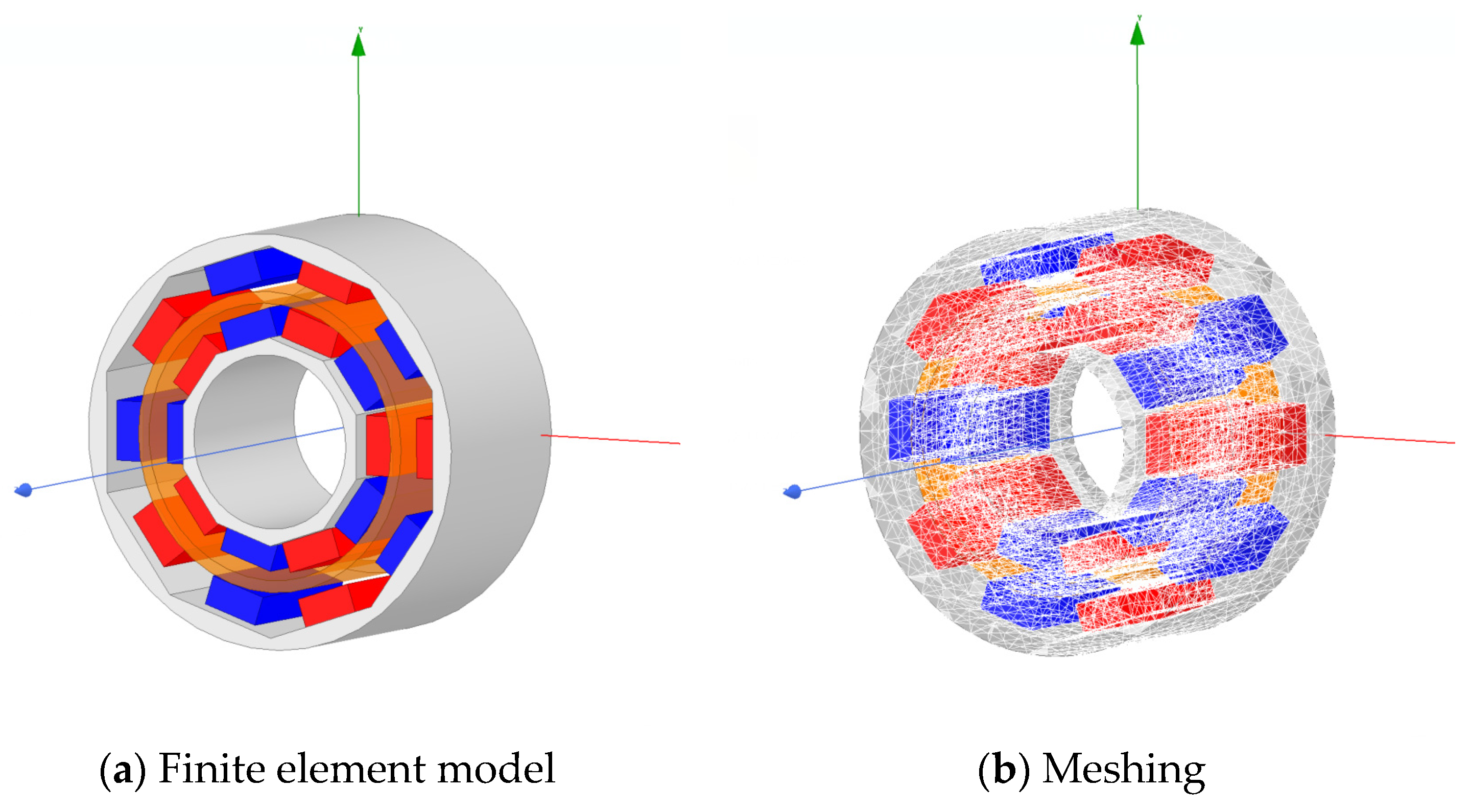
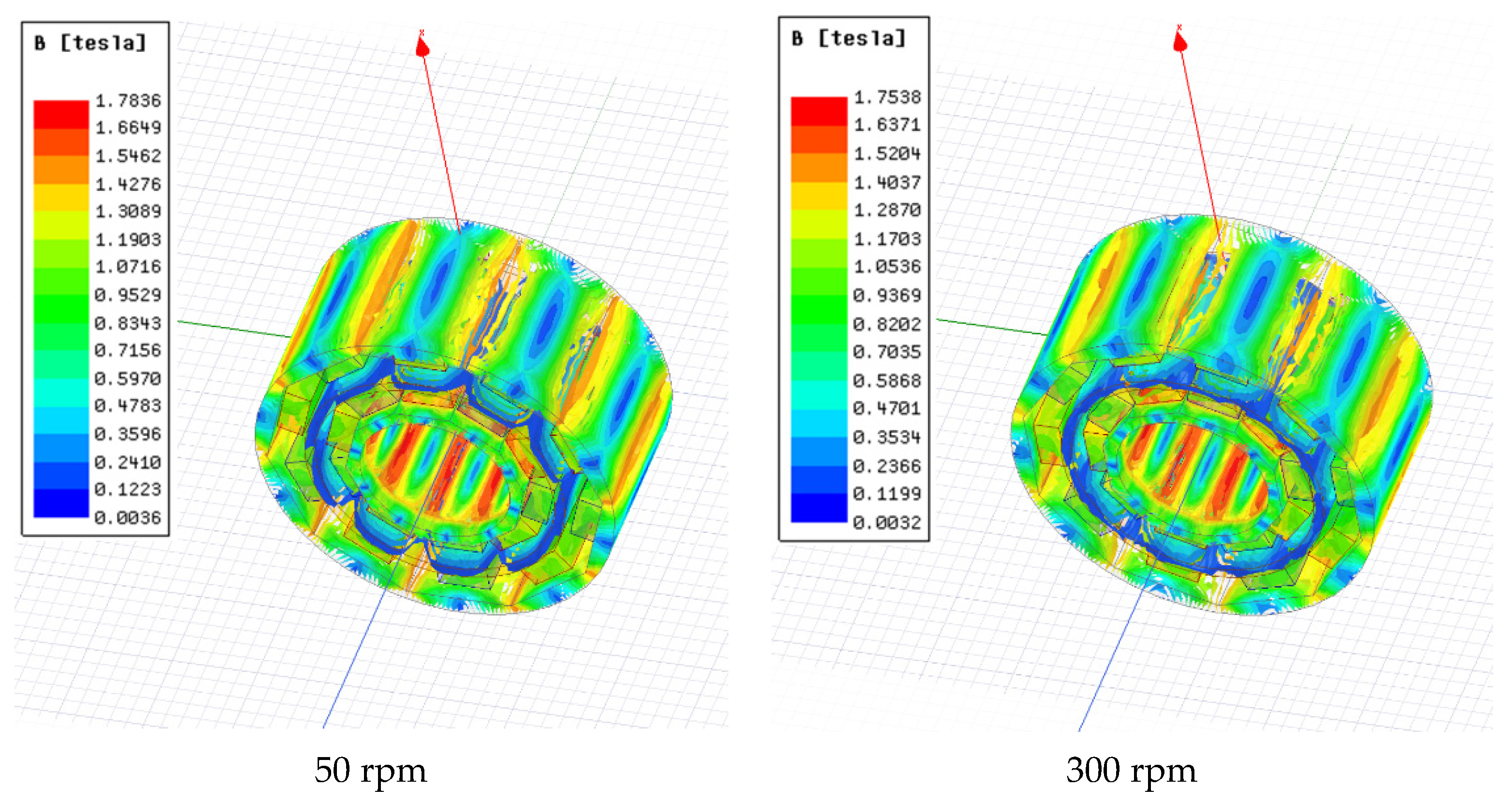
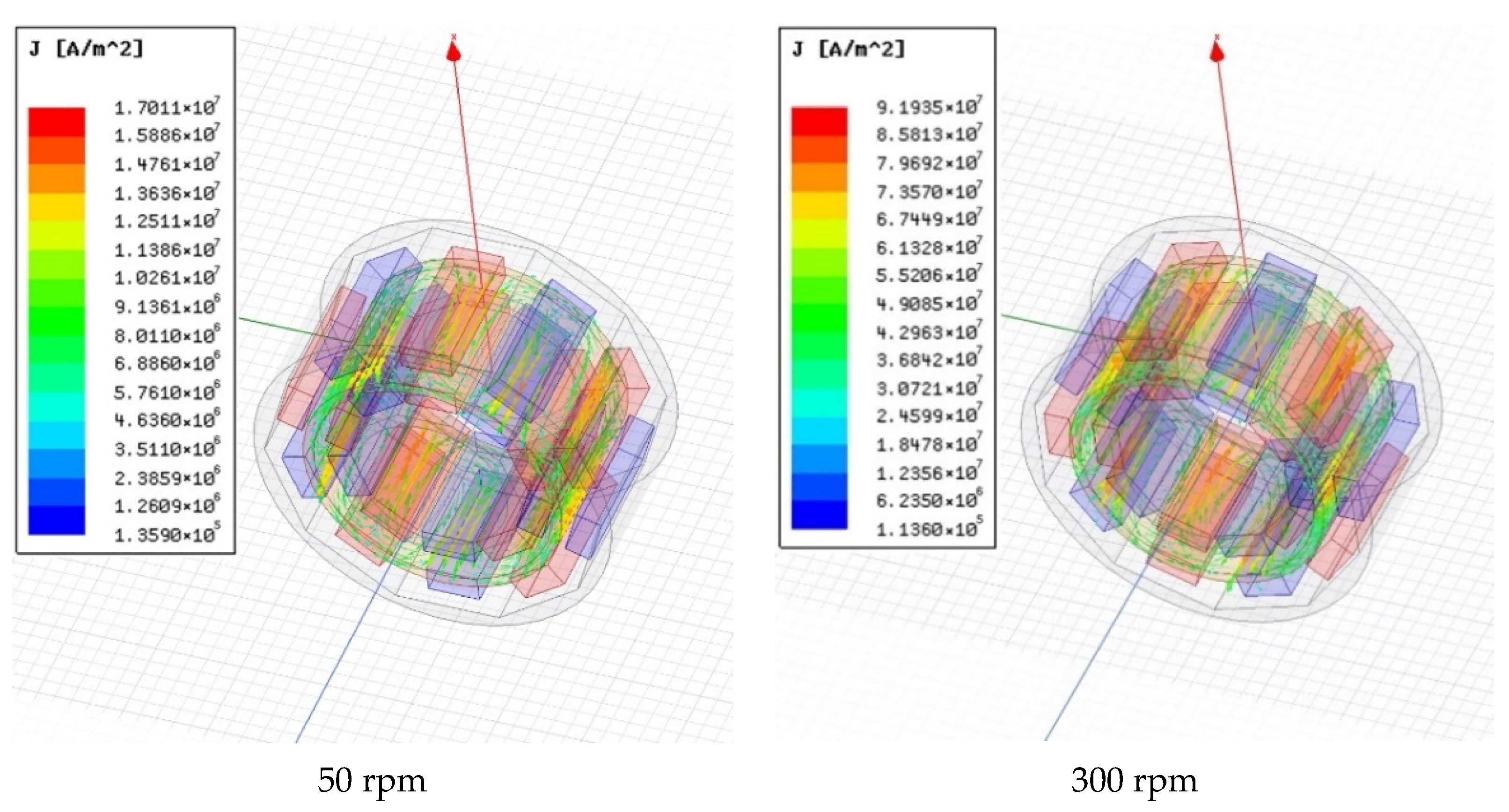
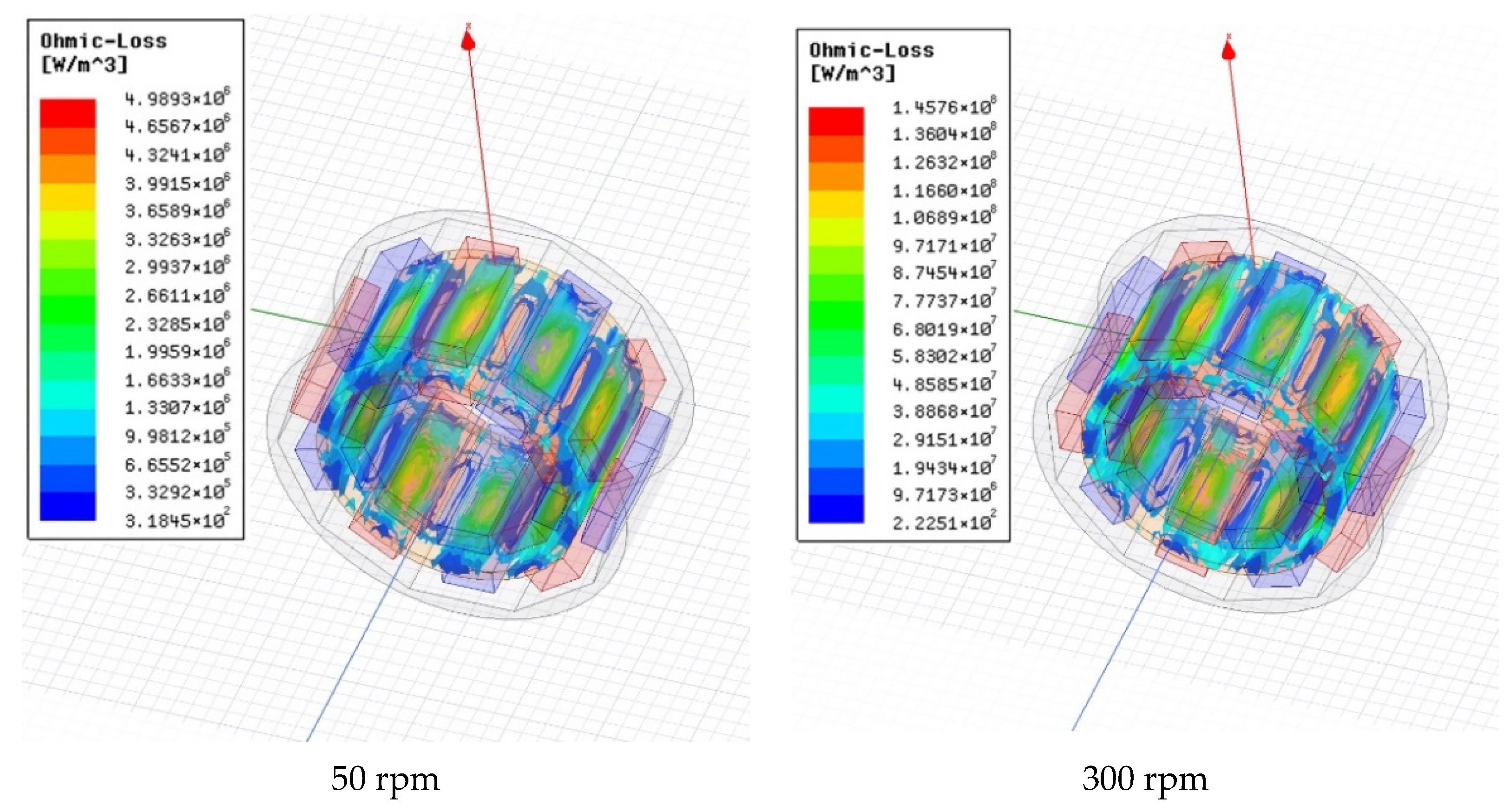
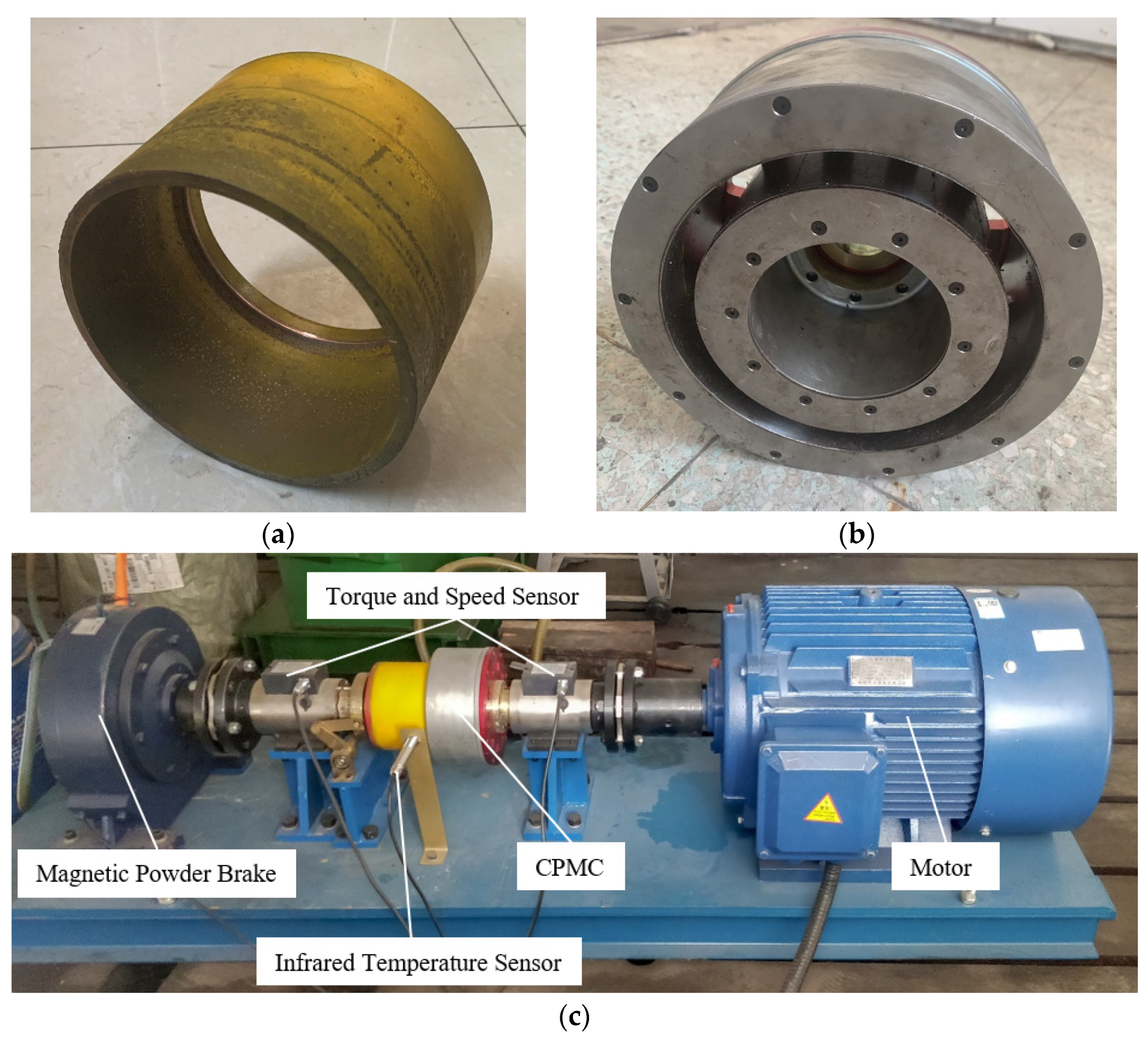
3. Simulation and Experimental Evaluation

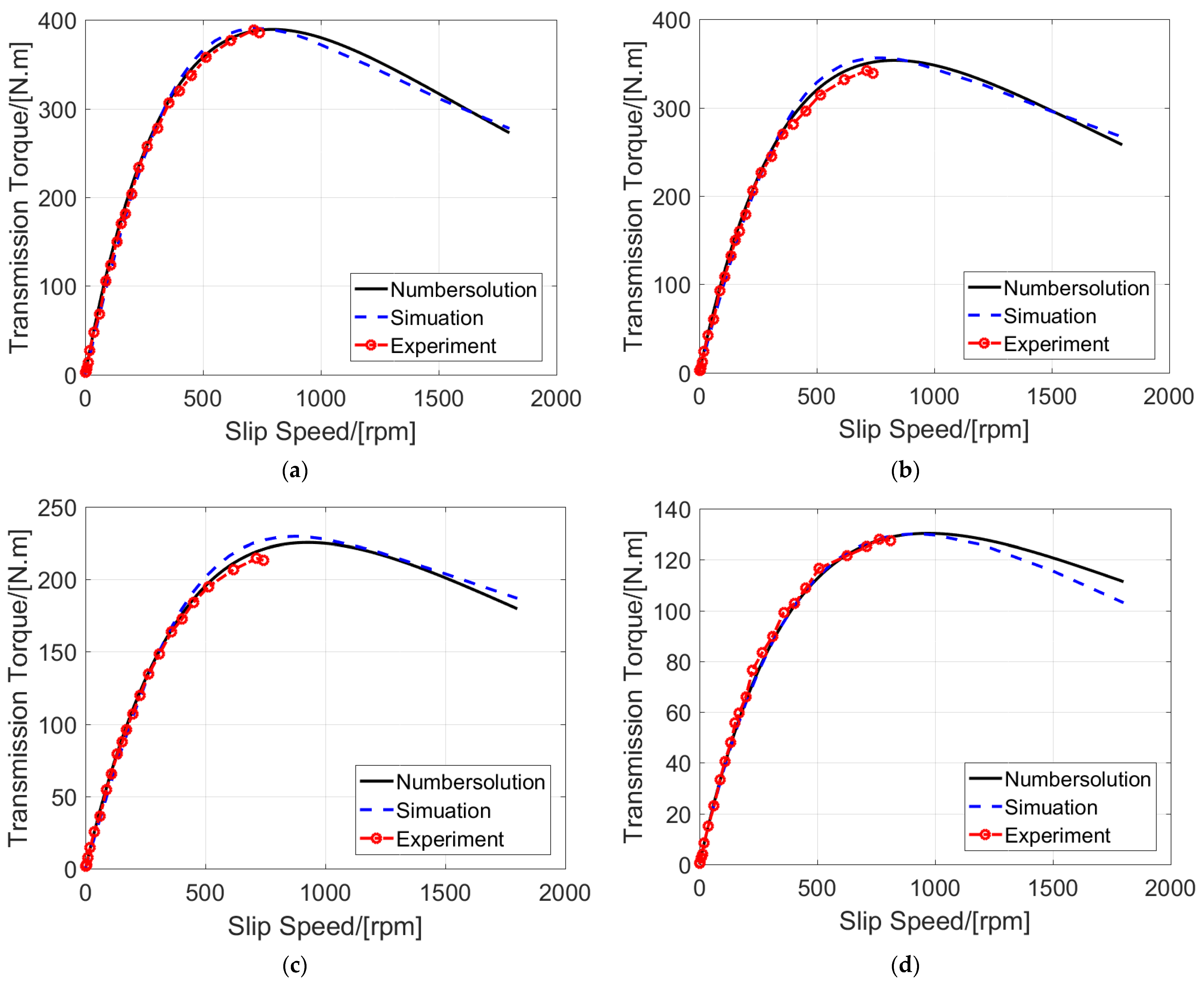
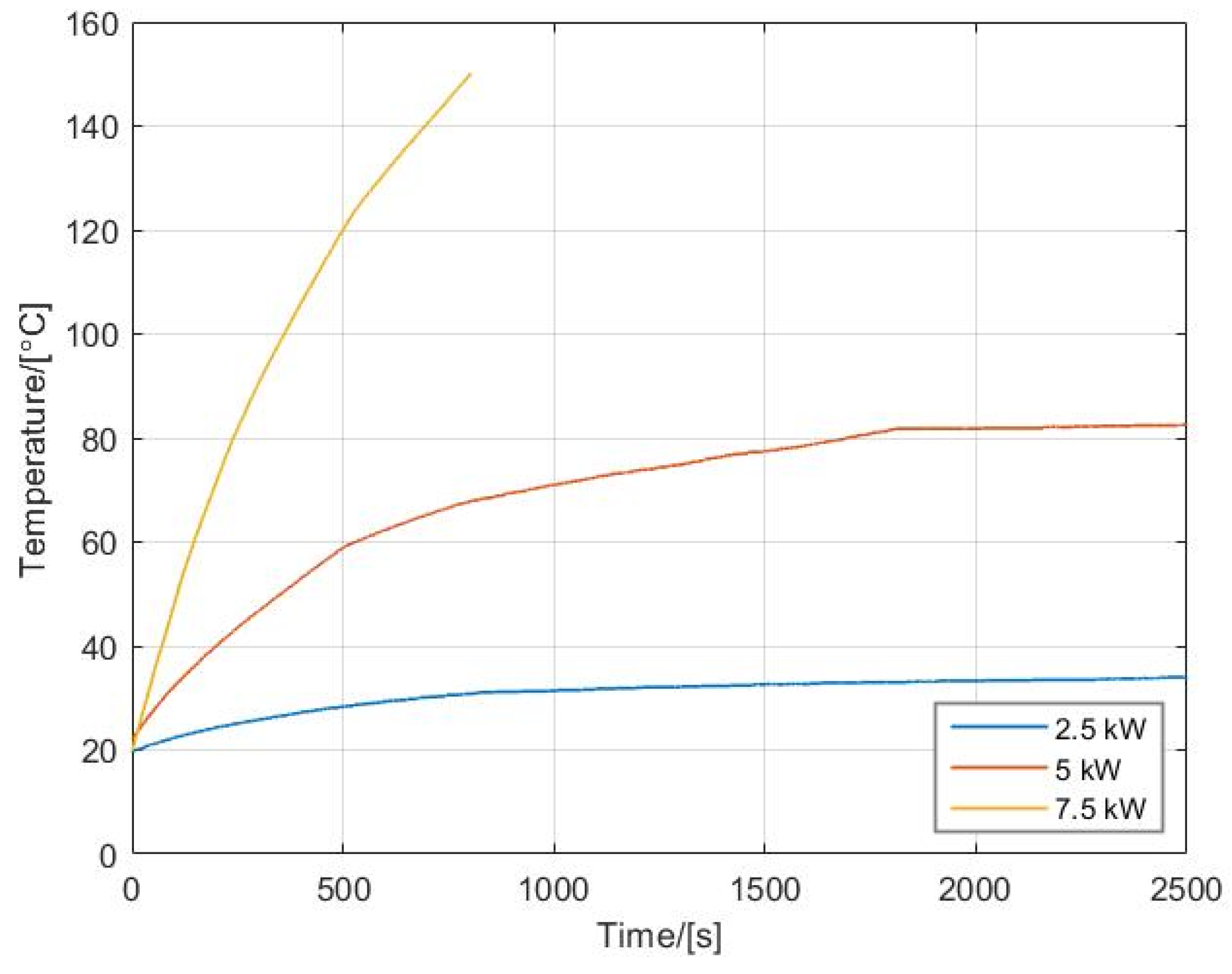
3.1. Simulation and Experimental Results

In this study, neodymium iron boron permanent magnets were used for permanent magnet coupling. The specific performance parameters of the permanent magnet are listed in

Table 1. Performance parameters of the permanent magnet.

Grade	Remanence	Coercive Force	Maximum Energy Product	Density	Curie Temperature	Maximum Work Temperature	Relative Permeability
N35SH	1.2 T	≥1592 kA/m	275 kJ/m3	7.55 g/cm3	320 °C	150 °C	1.05

. In addition, copper conductor tubes, aluminum frames, and inner and outer steel drums made of silicon steel with high magnetic permeability and low electrical conductivity were used.

The structural parameters of the permanent magnet coupling are listed in

Table 2. Structural parameters of permanent magnet coupling.

Parameters	Symbol	Value
Permanent magnet width (circumferential direction)	$a_m$	30 mm
Axial length of permanent magnet	$b_m$	100 mm
Permanent magnet thickness (radial direction)	$h_m$	15 mm
Permanent magnet logarithm	N	10
Distance between outer permanent magnet and center of circle	$l_{m1}$	78 mm
Distance between inner permanent magnet and center of circle	$l_{m2}$	53 mm
Outer diameter of steel drum	$r_{s1}$	104 mm
Inner diameter of steel drum	$r_{s2}$	48 mm
Axial length of conductor tube	$b_c$	120 mm
Average radius of conductor tube	$r_c$	72 mm
Conductor tube thickness	$h_c$	6 mm
Air gap thickness (radial distance between inner and outer permanent magnets)	$l_g$	10 mm

.

The FEM can discretize various different solution domains and can flexibly use element meshes of different structural shapes for division. Therefore, for models composed of multiple linear or nonlinear materials exhibiting complex structures and boundary conditions, the FEM can be applied to obtain a relatively accurate numerical solution. The material of the permanent magnet used in permanent magnet coupling is anisotropic. In addition, multiple materials are connected in a straight or curved manner, and the eddy currents are unevenly distributed. Thus, the FEM is suitable for solving the three-dimensional (3D) transient field of permanent magnet coupling to obtain its transmission torque.

The simulation software ANSYS Maxwell was used in this study to establish the FEA model [28]. The mathematical model of the magnetic vector A in the solution domain $\mathit{\Omega }$ is as follows:

$$\mathit{\Omega }:\frac{\partial }{\partial x}\left(\beta \frac{\partial \mathit{A}}{\partial x}\right)+\frac{\partial }{\partial y}\left(\beta \frac{\partial \mathit{A}}{\partial y}\right)+\frac{\partial }{\partial z}\left(\beta \frac{\partial \mathit{A}}{\partial z}\right)=0$$

(26)

The following three types of boundary conditions were set: (a) inner surface of the model as S_bc1; (b) interface between different media as S_bc2; and (c) side of the conductor along the radius of the driven rotor as S_bc3. The equations for these types of boundary conditions are as follows:

$$\{\begin{array}{c}{S}_{bc1}:\mathit{A}=0\hfill \\ S_{bc2}:{\left(\beta \frac{\partial \mathit{A}}{\partial n}\right)}_{s_{bc2}^{+}}={\left(\beta \frac{\partial \mathit{A}}{\partial n}\right)}_{s_{bc2}^{-}}\hfill \\ S_{bc3}:{\left(\beta \frac{\partial \mathit{A}}{\partial n}\right)}_{s_{bc3}^{+}}-{\left(\beta \frac{\partial \mathit{A}}{\partial n}\right)}_{s_{bc3}^{-}}=\mathit{J}\hfill \end{array},$$

(27)

where $\mathit{J}$ is the induced eddy current vector. In permanent magnet coupling, the main excitation source is the rotation of the permanent magnet, and the magnetic flux density vector B at each position in the solution domain is expressed as follows:

$$\mathit{B}=\nabla \times \mathit{A}$$

(28)

The electromagnetic induction principle is used to further calculate the torque dV (i.e., the differential element of volume) of the conductor tube, and the total torque is obtained by integration as follows:

$$\mathit{T}=\frac{1}{2}{{\displaystyle \int }}_V\left({{\displaystyle \int }}_{r_{c2}}^{r_{c1}}\mathit{J}\times \mathit{B}\times dr\right)dV,$$

(29)

where r_c1 and r_c2 are the outer and inner diameters of the conductor tube, respectively.

A simplified 3D model equivalent to the physical image of the permanent magnet coupling is shown in Figure 9a; the structures with a negligible impact on the computational result are ignored [29,30,31]. Considering the skin effect, tetrahedrons were used to divide the mesh, as shown in Figure 9b. The material parameters of each part of the permanent magnet coupling were imported, and the boundary conditions were set for the solution. FEA of the CPMC under two working conditions with a slip of 50 rpm (rated) and 300 rpm (high load) was performed; the results are shown in Figure 10, Figure 11 and Figure 12.

As shown in Figure 10, the area with the highest magnetic flux density in the conductor barrel is the area where the permanent magnet is mapped to the conductor tube. The maximum values are 1.85, 1.78, and 1.75 T when the slip is 20, 50, and 300 rpm, respectively. When the slip increases, the intensity of the magnetic induction decreases. This is because as the slip increases, the magnetic field generated by the conductor tube also increases, which causes the working point of the permanent magnet (Figure 6) to move toward the left; this, in turn, causes a reduction in the magnetic flux density.

As shown in Figure 11, the direction of the eddy current in the conductor tube conforms to the direction determined by the right-hand spiral rule, and the center of the eddy current is located at the center of the two adjacent permanent magnet mapping areas. The magnetic field generated by the eddy current interacts with that of the permanent magnet to generate torque. The area with the highest eddy current density in the conductor tube is where the permanent magnet is mapped to the conductor tube. When the slip is 20, 50, and 300 rpm, the maximum eddy current density is $5.2\times {10}^6,1.7\times {10}^7$, and $9.2\times {10}^7\mathrm{A}/{\mathrm{m}}^2$, respectively. The induced current significantly increases with the increase in the slip, and this, in turn, increases the induced magnetic field. Therefore, the torque between the permanent magnet and the conductor tubes increases. However, the increase in the induced eddy current also increases the eddy current loss. According to Figure 12, the maximum values of the eddy current loss density under the three slips are $4.10\times {10}^5,4.99\times {10}^6$, and $1.46\times {10}^8\mathrm{W}/{\mathrm{m}}^3$; an increase in the slip results in a significant increase in the eddy current loss. Hence, the heat generation of the permanent magnet coupling will significantly increase under high-load conditions.

The results of the FEA indicate that the eddy current that plays a decisive role in the torque transmission of the permanent magnet coupling is located in the area between the inner and outer permanent magnets (i.e., the mapping area of magnetic flux tube 1 on the conductor tube). The induced eddy current in the mapping areas of magnetic flux tubes 2 and 3 on the conductor tube is the smallest, two orders of magnitude lower than the maximum, and can be ignored in engineering calculations.

Figure 12 shows the test bench for the CPMC. A low-speed, high-torque motor is used as the driving element, which is connected to the CPMC via the input torque and speed sensor. The other side of the coupling is connected to the magnetic powder brake via the output torque and speed sensor. The engagement length between the conductor tube and the permanent magnet barrel can be adjusted using the screw structure. An infrared temperature sensor is placed outside the conductor tube to measure its temperature.

The results obtained using the computational model indicate that under the rated working condition of CPMC with a slip of 50 rpm, its torque is about 66 N.m, while the maximum torque is about 383 N.m, which is approximately 5.8 times the rated torque. As the input speed is the rated speed of the motor, and the relationship between the power of the PMC and the torque and input rotational speed n is given by $P=\frac{n\times T}{9550}$, it can be deduced that the power consumed by the PMC is proportional to its torque; thus, the operating power of the PMC exceeds five times its rated power when it is close to overload. Therefore, the rated power of the drive motor of the test bench must exceed five times the rated power of the PMC to test its performance under extreme working conditions. In most previous studies, the rated power of the drive motor used in the test bench was close to the power of the PMC [32,33]. Such power can only test the characteristics of the PMC when the slip rate is within 0.3; it cannot test the ultimate performance of the coupling. The rated power of the prototype tested in this test bench was 5 kW. To test its characteristics under extreme working conditions, we chose a three-phase asynchronous motor with a rated power of 30 kW as the drive motor. The parameters are shown in

Table 3. Parameters of three-phase asynchronous motor.

Type	Rate Power	Rate Current	Rate Voltage	Rate Rotational Speed
YE2 225M-6	30 kW	59.3 A	380 V	980 rpm

. The test bench could test the performance of the CPMC prototype in the full range of the slip rate from zero to one.

Speed torque sensors were arranged at both the input and output ends of the permanent magnet coupling to measure the differences between the input and output speeds and torques; that is, the differences in torque and speed are caused by mechanical friction and permanent magnet coupling, respectively. Thus, the error caused by mechanical friction can be eliminated.

Considering the working conditions with engagement lengths of 80, 60, 40, and 20 mm between the permanent magnet and conductor of the permanent magnet coupling, a comparison of the theoretical, simulation, and test data is presented in Figure 13.

In Figure 14, it can be seen that the transmission torque of the CPMC increases with the slip speed. When the slip speed approaches 800 rpm, the rate of increase in the transmission torque decreases; when the slip speed is approximately 800 rpm, the transmission torque reaches the maximum value; and when the slip speed continues to increase, the transmission torque decreases. This occurs because the increase in the slip speed causes an increase in the magnetic induction line cutting speed of the conductor tube as well as a gradual increase in the induced eddy current. Ampere’s force that is generated by the induced eddy current also increases gradually, leading to an increase in the transmission torque. However, when the slip speed is sufficiently high, the induced magnetic field formed by the induced eddy current will impose a reaction force on the original permanent magnet, which is reflected by the low-efficiency position of its working point. In addition, the skin effect gradually increases with the slip speed. Hence, the transmission torque gradually decreases when the slip speed is greater than 800 rpm.

Figure 14a–d indicate that for a constant slip speed and a decrease in the engagement length between the conductor tube and permanent magnet, the transmission torque of the permanent magnet coupling decreases. This is because the length of the magnetic field line cut by the conductor tube is shortened. In addition, the area where the conductor tube does not engage with the permanent magnet cannot generate eddy currents, leading to a decrease in the transmission torque. This characteristic of the CPMC can match the motor with different loads and limit the maximum transmission torque.

Furthermore, it is clear from Figure 14 that the theoretical computational model, the finite element simulation results, and the test results are in good agreement. Nevertheless, the finite element simulation results are more accurate. When the slip speed is greater than 800 rpm, the permanent magnet completely slips away from the conductor disk, and the torque sensor of the test fails. Therefore, the load is stalled, and the conductor tube connected to the load stops rotating. The power on the motor side is completely converted into heat generated by the induced eddy current, and the coupling increases dramatically. When the temperature rises to a certain level, it causes irreversible damage to the permanent magnet because it prevents the motor from stalling.

We tested the CPMC from startup to stable operation under transmission powers of 2.5, 5, and 7.5 kW and recorded the temperature. The corresponding temperature–time curve obtained is shown in Figure 15.

As shown in Figure 15, an increase in the transmission power increases the heating of the CPMC. However, the temperature increase is relatively small for the 2.5 kW working condition; after 1100 s, the temperature increased from 20 to 33 °C to reach thermal equilibrium and then stopped increasing. For the 5 kW working condition, it took a relatively long time to reach the thermal equilibrium state; specifically, the temperature initially increased to 83 °C, and after 1800 s, it reached a stable state. While the temperature of the CPMC continued to rise under the 7.5 kW working condition, the heat and heat dissipation could not be balanced; hence, to prevent the temperature of the CPMC from exceeding the Curie temperature of the permanent magnet, which would result in overheating and subsequent failure of the permanent magnet, the test bench was closed when the temperature increased to 150 °C after running for 800 s.

3.2. Discussion and Comparison

Kano et al. [5] proposed a PMC calculation model that uses the equivalent magnetic circuit approach. When the air gap of the PMC was 4 mm and the slip rate was 0.18, the error of their theoretical model was 9.7%, and when the air gap of the PMC was 8.5 mm and the slip rate was 0.15, the error was 11.3%. In short, the error of their calculation model increased with the air gap and slip rate. The theoretical model proposed by Cai and Wang [11] had the largest error at the maximum point, with a value of about 13%. The theoretical model proposed by Mohammadi and Mirsalim [34] had a higher accuracy under a low slip, but the error increased with the slip; the maximum error was 9% when the slip was 120 rpm. By contrast, the calculation model proposed in this article, when compared to the experimental values, has maximum errors of 2.3%, 2.5%, 3.6%, and 8.7% under engagement lengths of 80 mm, 60 mm, 40 mm, and 20 mm, respectively. The error increases with reductions in the engagement length, but compared with the above theoretical models, the theoretical model proposed in this article has higher accuracy.

The CPMC transmitted torque through the slip speed, and its torque density varied with the slip speed. The test results indicate that the torque densities of the CPMC were 9 Nm/kg when the slip speeds were 40 rpm.

Table 4. Comparison of the torque density of various couplings.

Devices/Status	CPMC/40 rpm	AS-PMECC/40 rpm	Magnetic Torque Limiter/20 °C	RF-CPMC	FC-CPMC
Torque Density	9 Nm/kg	6 Nm/kg	20 Nm/kg	80 Nm/kg	60 Nm/kg

compares the torque density of an adjustable-speed permanent magnet eddy current coupling (AS-PMECC) at 40 rpm [22], an aeronautical magnetic torque limiter at 20 °C [35], a radial flux cylindrical permanent magnet coupling (RF-CPMC), and a flux-concentrating cylindrical permanent magnet coupling (FC-CPMC) based on a reference study [36].

It can be seen from Table 4 that the torque density of the AS-PMECC at 40 rpm is the lowest, and that of the CPMC at 40 rpm is slightly higher. However, compared to the magnetic torque limiter, RF-CPMC, and FC-CPMC, the torque density is much smaller for the CPMC and AS-PMECC.

In Table 4, the CPMC and AS-PMECC are asynchronous PMCs, which provides them with the inherent advantages of speed adjustment, soft start, and overload protection. In contrast, the other three are synchronous PMCs, which provides better permanent magnet utilization than asynchronous PMC.

4. Conclusions

In this study, we established a theoretical computational model of CPMC and an FEA model, built a test bench, and carried out simulation analysis and experimental investigation of CPMC. The following conclusions can be drawn.

(1) In accordance with the basic laws of magnetic circuits, this study used the magnetic field division method to divide the magnetic circuit of a CPMC into multiple magnetic flux tubes. Then, based on the structure of the coupling, an equivalent magnetic circuit model of the permanent magnet coupling was established using the equivalent magnetic circuit method. The working point of the permanent magnet was determined from the recovery curve, and the skin effect was found to be equivalent to an increase in the resistivity of the conductor tube. The intensity of the induced eddy current in the conductor tube was calculated based on the principle of electromagnetic induction. The transmission torque of the permanent magnet coupling was obtained using Ampere’s law, and a theoretical computational model of the transmission torque was established.

(2) In accordance with the computational model, the established FEA model, and test bench, and through FEA and experimental verification, we proved that the error of the model meets the requirements of engineering calculations. The error of the theoretical model increases with reductions in the engagement length, and, compared to the experimental results, the maximum error is 8.7%. Compared with several existing theoretical models, the accuracy of the proposed model is higher, and it is easy to use for calculations, which ensures good practicability. Compared with the CPMC of the traditional single-sided type, the CPMC under this model has the advantages of a high working efficiency and saving the permanent magnet space, which enable it to have a good application prospect.

(3) The temperatures under the 2.5, 5, and 7.5 kW working conditions were tested and recorded, and a temperature–time curve was plotted. The temperature–time curve shows that under the 7.5 kW working condition, the heating and heat dissipation of the CPMC cannot be balanced. Consequently, the temperature of the CPMC continues to rise, resulting in the inability to work for a long time. Therefore, the temperature is an important factor that limits the high-load performance of CPMC. In future work, the influence of the temperature on the performance of permanent magnets and permanent magnet couplings will be studied to implement this model in applications under high-load conditions.

The novelty of this study is the consideration of the working point of the permanent magnet under the actions of the external magnetic circuit, air gap magnetic flux leakage, and skin effect. In addition, the complete torque characteristics of the permanent magnet coupling were tested using a high-power motor. The theoretical computational model herein has a certain guiding significance for the design, model selection, manufacturing, and future research of CPMC. In addition, CPMC has the functions of speed adjustment, soft start, and overload protection; thus, the work presented in this article can also provide certain ideas for research in the motor control field.

References

- Li, Y.; Hu, Y.; Song, B.; Mao, Z.; Tian, W. Performance analysis of conical permanent magnet couplings for underwater propulsion. J. Mar. Sci. Eng. 2019, 7, 187. [Google Scholar] [CrossRef] [Green Version]
- Rhyu, S.-H.; Khaliq, S.; Baek, C.W.; Ha, Y.C. Optimal design and static performance analysis of permanent magnet coupling for chemical pump application. J. Magn. 2020, 25, 64–69. [Google Scholar] [CrossRef]
- Cao, R.; Cheng, M.; Hua, W. Investigation and general design principle of a new series of complementary and modular linear FSPM motors. IEEE Trans. Ind. Electron. 2013, 60, 5436–5446. [Google Scholar] [CrossRef]
- Zhu, Z.N.; Meng, Z. 3D analysis of eddy current loss in the permanent magnet coupling. Rev. Sci. Instrum. 2016, 87, 074701. [Google Scholar] [CrossRef]
- Kano, Y.; Kosaka, K.; Matsui, N. A simple nonlinear magnetic analysis for axial-flux permanent-magnet machines. IEEE Trans. Ind. Electron. 2010, 57, 2124–2133. [Google Scholar] [CrossRef]
- Nguyen, T.D.; Tseng, K.; Zhang, S.; Nguyen, H.T. A novel axial flux permanent-magnet machine for flywheel energy storage system: Design and analysis. IEEE Trans. Ind. Electron. 2011, 58, 3784–3794. [Google Scholar] [CrossRef]
- Canova, A.; Freschi, F.; Gruosso, G.; Vusini, B. Genetic optimisation of radial eddy current couplings. COMPEL-Int. J. Comput. Math. Electr. Electron. Eng. 2005, 24, 767–783. [Google Scholar] [CrossRef]
- Bracikowski, N.; Hecquet, M.; Brochet, P.; Shirinskii, S.V. Multi-physics modeling of a permanent magnet synchronous machine by using lumped models. IEEE Trans. Ind. Electron. 2012, 59, 2426–2437. [Google Scholar] [CrossRef]
- Hsieh, M.; Hsu, Y. A generalized magnetic circuit modeling approach for design of surface-permanent magnet machines. IEEE Trans. Ind. Electron. 2012, 59, 779–792. [Google Scholar] [CrossRef]
- Mohammadi, S.; Mirsalim, M.; Sadegh, V.Z. Nonlinear modeling of eddy-current couplers. IEEE Trans. Energy Convers. 2014, 29, 224–231. [Google Scholar] [CrossRef]
- Cai, C.S.; Wang, J.H. Electromagnetic properties of cylinder permanent magnet eddy current coupling. Int. J. Appl. Electromagn. 2017, 54, 655–671. [Google Scholar] [CrossRef]
- Li, Y.; Cai, S.; Yao, J.; Cheng, J. Influence analysis of structural parameters on transfer characteristics of high-power permanent magnet eddy-current coupling. China Mech. Eng. 2017, 28, 1588–1592. [Google Scholar]
- Zheng, D.; Guo, X.F. Analytical prediction and analysis of electromagnetic-thermal fields in PM eddy current couplings with injected harmonics into magnet shape for torque improvement. IEEE Access 2020, 8, 60052–60061. [Google Scholar] [CrossRef]
- Meng, G.Y.; Niu, Y.H. The torque research for permanent magnet coupling based on ansoft Maxwell transient analysis. Appl. Mech. Mater. 2013, 423, 2014–2019. [Google Scholar] [CrossRef]
- Yuan, W.Q.; Liu, Y.; Li, D.; Meng, G.Y. Research on Overloading Protection of Permanent Magnetic Coupler in Coal Mine. Appl. Mech. Mater. 2014, 597, 492–497. [Google Scholar] [CrossRef]
- Cao, Y.; Li, X.; Liu, W. The Analysis of Thermal Magnetic Coupling of Tubular Permanent Magnetic Coupler. J. Phys. Conf. Ser. 2020, 1550, 042044. [Google Scholar] [CrossRef]
- Roters, H.C. Electromagnetic Devices; John Wiley & Sons: Hoboken, NJ, USA, 1941. [Google Scholar]
- Pfister, P.D.; Perriard, Y. Slotless permanent-magnet machines: General analytical magnetic field calculation. IEEE Trans. Magn. 2011, 47, 1739–1752. [Google Scholar] [CrossRef]
- Matsumoto, T.R.; Chabu, I. Resistive torque in permanent magnet couplings operating through a conductive wall. COMPEL-Int. J. Comput. Math. Electr. Electron. Eng. 2017, 36, 1120–1133. [Google Scholar] [CrossRef]
- Mohammadi, S.; Mirsalim, M.; Sadegh, V.Z.; Talebi, H.A. Analytical modeling and analysis of axial-flux interior permanent-magnet couplers. IEEE Trans. Ind. Electron. 2014, 61, 5940–5947. [Google Scholar] [CrossRef]
- Dai, X.; Liang, Q.; Cao, J.; Long, Y.; Mo, J.; Wang, S. Analytical modeling of axial-flux permanent magnet eddy current couplings with a slotted con-ductor topology. IEEE Trans. Magn. 2016, 52, 1–15. [Google Scholar]
- Li, Y.; Lin, H.; Tao, Q.; Lu, X.; Yang, H.; Fang, S.; Wang, H. Analytical analysis of an adjustable-speed permanent magnet eddy-current coupling with a non-rotary mechanical flux adjuster. IEEE Trans. Magn. 2019, 55, 8000805. [Google Scholar] [CrossRef]
- Liu, D.; Tang, Y. Calculation of permanent magnetic working points of polarity magnetic systems based on superposition. Mar. Electr. Electron. Eng. 2010, 30, 45–49. [Google Scholar]
- Gao, Y.; Huang, J.; Zhang, S. Optimal calculating on working point of the permanent magnet. AER-Adv. Eng. Res. 2015, 27, 1026–1040. [Google Scholar]
- Belevitch, V. Lateral skin effect in a flat conductor. Philips. Tech. Rev. 1971, 6–8, 221–231. [Google Scholar]
- Jablonski, P.; Szczegielniak, T.; Kusiak, D.; Piatek, Z. Analytical-numerical solution for the skin and proximity effects in two parallel round conductors. Energies 2019, 12, 3584. [Google Scholar] [CrossRef] [Green Version]
- Kahl, G.D.; Weber, F.N. Circuit analogy for skin effects in conductors. Am. J. Phys. 1971, 39, 321. [Google Scholar] [CrossRef]
- Yamazaki, K.; Abe, A. Loss Analysis of interior permanent magnet motors considering carrier harmonics and magnet eddy currents using 3-D fem. In Proceedings of the IEEE International Electric Machines & Drives Conference 2007, Antalya, Turkey, 3–5 May 2007; pp. 904–909. [Google Scholar]
- Zhang, H.; Zou, J.; Zhu, H. The numerical calculation of eddy-current field and temperature field for insulation shell of permanent magnet shaft coupling. In Proceedings of the International Conference on Electrical Machines and Systems 2007, Seoul, Korea, 8–11 October 2007; pp. 1397–1401. [Google Scholar]
- Tiang, T.L.; Ishak, D.; Lim, C.P.; Jamil, M.K.M. A comprehensive analytical subdomain model and its field solutions for surface-mounted permanent magnet machines. IEEE Trans. Magn. 2015, 51, 8104314. [Google Scholar] [CrossRef]
- Knight, A.M.; Zhan, Y. Identification of flux density harmonics and resulting iron losses in induction machines with nonsinusoidal supplies. IEEE Trans. Magn. 2008, 44, 1562–1565. [Google Scholar] [CrossRef]
- Yang, X.; Liu, Y.; Wang, L. An improved analytical model of permanent magnet eddy current magnetic coupler based on electromagnetic-thermal coupling. IEEE Access 2020, 8, 95235–95250. [Google Scholar] [CrossRef]
- Yang, X.; Liu, Y.; Wang, L. Nonlinear modeling of transmission performance for permanent magnet eddy current coupler. Math. Probl. Eng. 2019, 2019, 2098725. [Google Scholar] [CrossRef]
- Mohammadi, S.; Mirsalim, M. Double-sided permanent-magnet radial-flux eddy-current couplers: Three-dimensional analytical modelling, static and transient study, and sensitivity analysis. IET Electr. Power Appl. 2013, 7, 665–679. [Google Scholar] [CrossRef]
- Cristache, C.; Diez-Jimenez, E.; Valiente-Blanco, I.; Sanchez-Garcia-Casarrubios, J.; Perez-Diaz, J.L. Aeronautical magnetic torque limiter for passive protection against overloads. Machines 2016, 4, 17. [Google Scholar] [CrossRef] [Green Version]
- Park, J.; Paul, S.; Chang, J.; Hwang, T.; Yoon, J. Design and comparative survey of high torque coaxial permanent magnet coupling for tidal current generator. Int. J. Electr. Power Energy Syst. 2020, 120, 105966. [Google Scholar] [CrossRef]
Publisher’s Note: MDPI stays neutral with regard to jurisdictional claims in published maps and institutional affiliations. |
© 2021 by the authors. Licensee MDPI, Basel, Switzerland. This article is an open access article distributed under the terms and conditions of the Creative Commons Attribution (CC BY) license (https://creativecommons.org/licenses/by/4.0/).