Abstract
The computing resources of today’s smartphones are underutilized most of the time. Using these resources could be highly beneficial in edge computing and fog computing contexts, for example, to support urban services for citizens. However, new challenges, especially regarding job scheduling, arise. Smartphones may form ad hoc networks, but individual devices highly differ in computational capabilities and (tolerable) energy usage. We take into account these particularities to validate a task execution scheme that relies on the computing power that clusters of mobile devices could provide. In this paper, we expand the study of several practical heuristics for job scheduling including execution scenarios with state-of-the-art smartphones. With the results of new simulated scenarios, we confirm previous findings and better comprehend the baseline approaches already proposed for the problem. This study also sheds some light on the capabilities of small-sized clusters comprising mid-range and low-end smartphones when the objective is to achieve real-time stream processing using Tensorflow object recognition models as edge jobs. Ultimately, we strive for industry applications to improve task scheduling for dew computing contexts. Heuristics such as ours plus supporting dew middleware could improve citizen participation by allowing a much wider use of dew computing resources, especially in urban contexts in order to help build smart cities.
1. Introduction
Smartphones have increasing capabilities of processing information, which typically are underutilized [1,2]. Cities (and citizens) could benefit from such a plethora of underutilized resources if these were properly orchestrated. Any person carrying a smartphone could contribute with valuable resources to help cities grow and to manage them in a more sustainable way. For instance, anyone may help to improve urban road maintenance by collecting pavement data [3]. Participatory platforms have been proposed to enable people to voluntarily contribute data sensed with their personal mobile devices [4,5].
Cities generate vast amounts of data for different smart city applications through Internet of Things (IoT) sensors and surveillance cameras [6,7]. Processing locally sensed data can be done in different but not necessarily mutually exclusive ways, for instance, using distant cloud resources, offloaded to proximate fog servers, or with the help of devices with computing capabilities within the data collection context, e.g., with smartphones. This latter architectural option has been considered as an attractive self-supported sensing and computing scheme [8]. In addition, hybrid and volunteer-supported processing architectures were proposed to avoid overloading resource-constrained devices [9]. Depending on the adopted approach—hybrid or self-supported—effectively managing smartphones’ limited energy and heterogeneous computing capabilities requires more research [10].
In a previous work [1], we proposed baseline heuristics to perform such resource management for a variant of self-supported sensing and a computing scheme where data collected in a local context is processed by a group of smartphones within the same context. We call that a “dew context” to continue with the cloud/fog metaphor used to describe a layered computing infrastructure.
Complementary, in this work, we subject these baseline heuristics to new execution scenarios, now considering simulated dew contexts with modern smartphone profiles—battery traces and benchmark results from recent smartphone models. Additionally, we go beyond simulating synthetic jobs load by benchmarking CPU usage and inference time of a Tensorflow lite state-of-the-art model trained for recognizing a set of generic objects. Throughout this new set of experiments we shed some light on the viability of distributing jobs at the edge using smartphones for AI-based data stream processing applications in smart cities, which is another major difference with respect to [1].
Specifically, the contributions introduced by this paper are:
- 1.
- We evaluate state-of-the-art practical load balancing heuristics for dew computing [1] but using performance parameters and battery traces from recent smartphone models. This helps to ensure the practical significance of such heuristics.
- 2.
- We compare results of current and previous experiments to refine our findings on the heuristics’ performance;
- 3.
- We illustrate the practical benefits of adopting our multi-smartphone computing approach versus single-smartphone computing through a realistic scenario, centered around a real Android application for AI-based object detection that might serve as a kernel for implementing many edge-powered smart city applications.
This paper is organized as follows. Section 2 discusses related work. Then, Section 3 provides a motivating example. Section 4 presents the studied scheduling heuristics. Section 5 describes the evaluation methodology and experimental design, while Section 6 gives an overview of metrics and results. In Section 7, we present an experiment simulating AI-based video processing. A summary of results and practical challenges are discussed in Section 8, while Section 9 concludes and points to future work.
2. Related Work
The exploitation of computing resources provided by smart devices in dew computing contexts—i.e., where both data collection and processing happen at the edge of the network—introduces new challenges in terms of job scheduling algorithms [10]. Since smart devices rely on batteries as their main power source, one of the challenges is to manage the remaining energy of resource provider nodes in the network. Hence, the impact of a given job execution schedule on a device’s future battery level must be considered. This involves targeting the maximization of completed jobs without exceeding the node’s energy availability.
There are at least two approaches for pursuing this objective. One models job scheduling as an optimization problem. Chen et al. [11], Ghasemi-Falavarjani et al. [12], Wei et al. [13] suggested to include a device’s remaining energy as a constraintin the problem formulation, i.e., while exploring feasible solutions, the energy employed in executing jobs must not exceed the available energy on the devices’ batteries. To tailor input variables of algorithms following this approach, it is necessary to have accurate job energy consumption data, which are rarely available. To obtain such data in the general case, a detailed quantification of resource demands are needed, which, in turn, vary according to device characteristics. Given the wide variability of device models on the market (cf., e.g., work by Rieger and Majchrzak [14]), it is unrealistic to assume homogeneous device clusters. If not pre-computed, scheduling input should be obtained while converting a data stream into jobs to be processed.
The other approach does not require energy-related job details. It performs load balancing based solely on node characteristics. Hirsch et al. [15] combined the last known battery level with a function including different performance scores, which rates the capability of a device to successfully complete the last arrived job. Jobs are scheduled by following an online approach, i.e., upon each job arrival, the scheduling logic creates a ranking by evaluating the function for all candidate devices, and the job is assigned to the one ranked best.
Resource heterogeneity imposes further challenges that scheduling algorithms in dew computing contexts must deal with. The co-existence of smart devices that belong to the same or different generations, equipped with hardware able to render dissimilar computing and data transfer throughput, should not be ignored when including them as first-class resource providers. The authors of Yaqoob et al. [16] considered the number of cores, speed, and CPU workload, which are evaluated by the proposed heuristics when allocating computing-intensive tasks to mobile devices. The authors of Hirsch et al. [15] considered heterogeneity by differentiating the nodes’ computing capabilities via their MFLOPS indicator, which is a common metric in scientific computing to rate processor speed when executing floating-point operations. All in all, the heuristics by Yaqoob et al. [16] recognize resource heterogeneity related to computing capability only. For stream processing applications, where data transfer under varying delay and energy consumption of wireless communication is present, new practical online heuristics are necessary to deal with both node computing and communication heterogeneity.
3. Motivating Example
Smart cities integrate multiple sources of information and process massive volumes of data to achieve efficient solutions and monitor the state of a wide range of common issues, including maintenance of public spaces and infrastructure or the security of citizens, just to mention two of them. Ultimately, they contribute to societal security [17]. Participatory sensing platforms encourage citizens to contribute incidents data, such as geolocalized photos, videos, and descriptions that have to be analyzed, filtered, and prioritized for proper treatment. This requires a data processing infrastructure and depends on the citizens’ willingness to manually enter or record data.
A proactive way to gather relevant data could be installing a dedicated sensor and processing infrastructure. However, to reduce fixed costs and to avoid the congestion of communication networks with a high volume of raw data captured [18], a hybrid approach that exploits near-the-field, ubiquitous computing power of smart mobile devices is feasible. By analyzing a city’s dynamics, it is not hard to identify places where citizens are regularly connected to the same local area network with their smartphones, e.g., small parks or public transport. Suppose that citizens in such a context agree to contribute processing power, even though they may not like to provide data sensed with their devices. However, these may be used to filter and identify relevant information from data streams captured by sensors cleverly positioned within the context, and connected to the same network as nearby mobile users.
Consider, for instance, passengers riding a bus, where smartphones receive data via their WiFi connections. These may be samples of environmental sounds or images captured with devices that have been specifically installed in the bus for, e.g., real-time sensing of noise pollution, detecting pavement potholes, counting trees or animals, or whatever information may be useful for a smart city to forecast events, schedule repairs, or public space maintenance duties. The smartphones could be used, on a voluntary basis, for pre-processing such data before it is transferred to the distant cloud in a curated and reduced form. Pre-processed data, in turn, could be used to feed Internet-accessible, real-time heatmaps summarizing such information so that decision-makers can act promptly and accordingly. In terms of the hardware resources to be exploited, the computations required to do so might range from medium-sized, CPU-intensive ones, such as finding patterns in digitized sound streams, to complex CPU/GPU-intensive tasks such as detecting or tracking objects from image streams using deep neural networks. Nowadays, it is not surprising to find affordable smartphones on the market with eight-core processors and GPUs capable of running deep learning frameworks such as Tensorflow (https://www.tensorflow.org/ accessed on 18 August 2021).
How to efficiently and fairly balance data processing among available smartphones in a dew context is challenging, though. This essentially stems from the singularities that characterize smartphones [19], namely user mobility, lack of ownership, and exhaustible resources. Smartphones are inherently mobile devices and their users may enter/leave the dew context in unpredictable ways, constraining the time window within which computations can be submitted and successfully executed on a device. Failure to obtain task results from a leaving device intuitively forces the scheduler to either discard these results, which harms effectiveness from the application standpoint, or re-submitting the associated tasks to alternative devices, which harms application throughput. Moreover, lack of ownership means that from the perspective of a data processing application, smartphones are non-dedicated computing resources, of course. Resources such as CPU/GPU time, memory, storage, and network bandwidth are shared with user processes and mobile applications. Hence, any dew scheduler must ensure that data processing tasks do not significantly degrade the performance of native applications and user experience, otherwise users might become reluctant to contribute or keep contributing their computing resources in dew contexts. Lastly, the serving time of a mobile device is limited both by the energy level of its battery at the time it enters the dew context, and the rate at which energy is consumed by the mobile device, which depends on several factors including screen brightness level, user applications and system services being executed, battery inherent efficiency, and so on. Not only computing capabilities (e.g., CPU/GPU speed) are important for distributing dew tasks, but also energy availability/battery efficiency. Of course, a dew scheduler should not exhaust a mobile device’s energy since this would also discourage users to process dew tasks.
4. Load Balancing Heuristics
Figure 1 depicts an overview of a dew context, a distributed computing mobile cluster (in this case, operating inside a bus) for processing jobs generated locally. When close to the dew context local area network, mobile devices are enlisted to contribute with computing resources by registering themselves with the proxy [20]. In the example, the proxy is an on-chip-pc integrated circuit. The proxy balances the jobs processing load with a heuristic that sorts the devices’ appropriateness using some given criterion. The best ranked node is assigned with the incoming job and the ranking is re-generated upon each job arrival.
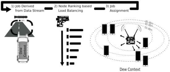
Figure 1.
The dew context.
We propose and evaluate practical heuristics to sort devices, which combine easy-to-obtain device and system performance information. One of these is AhESEAS, an improvement to the ESEAS (Enhanced Simple Energy-Aware Scheduler) [20]. Another heuristic is ComTECAC, which was inspired by criteria targeting nodes’ fair energy spending [21]. In the following, we provide details of the formulation of these novel criteria to rank resource provider devices.
AhESEAS: the Ahead Enhanced Simple Energy Aware Scheduler is a criterion that combines a device’s MFLOPS, its last reported battery level (SOC) and a counter of assigned jobs, in the same way as the ESEAS [20] formula, with the exception of a change in the semantics of the last-mentioned counter. While in ESEAS the counter of assigned jobs is updated after the job input has been completely received by the node, in AhESEAS such an update occurs before, i.e., just after a node is selected for executing a job. By issuing an immediate counter update, i.e., without waiting for job input transferring time, gives AhESEAS rapid reaction to fast and continuous job generation, typical in stream processing applications. To differentiate the semantic change and to avoid confusion with the ESEAS formula, we have renamed of ESEAS by in the AhESEAS formula (and adding 1 to avoid that the denominator may become 0):
ComTECAC: the Computation-Communication Throughput and Energy Contribution Aware Criterion utilizes indicators of a node’s computing and communication capabilities, as well as its energy spent for executing dew jobs, which is implemented with battery level updates reported by nodes. Ranking heuristics using ComTECAC determine the best-ranked node not only using a queued jobs component, but also with an energy contribution component. Thus, the load is evenly distributed among nodes, avoiding that strong nodes drain their batteries too much and earlier than weak nodes. This heuristic’s formula is:
where:
- and have the same semantics as in AhESEAS.
- is calculated as , where relates node RSSI (received signal strength indicator) with Joules spent per KB of data transferred. is pre-computed and retrieved from a look-up table for a given RSSI value (see Table 2).
- is a normalized value of the last reported battery level.
- is a normalized value that accounts for the energy contributed by a device since it joined the mobile cluster. This value is updated upon each battery level drop reported by a node. The sub-formula to calculate it is , where is the node battery level when it joined the cluster.
The rationale that led us to propose node ranking formulas based mainly on node information is that such information is easy to systematize providing that node resources/capabilities can be determined through the specifications of the constituent hardware parts, either via manufacturer data (e.g., battery capacity) or comparisons with other nodes through benchmark suites [22,23,24,25]. For scheduling purposes, the update frequency of such information in our approach would depend on the existence of new device models or benchmarks on the market. Node information can be collected once, systematized, and reused many times. In contrast, except for special-purpose systems running jobs from very specific applications, scheduling logic that uses job information as input—e.g., job execution time—is difficult to generalize, in principle, due to the impossibility to accurately estimate the job execution time of any possibly given job [26]. In the dew contexts studied in this paper, where nodes are battery-driven, balancing load to maintain as many nodes ready for service for as long as possible, is a strategy that maximizes the parallel execution of independent jobs, which in turn aims at reducing makespan. The more cores are available, the more jobs execution can be expected to progress in parallel. For the proposed node ranking formulas, we adopt a fractional shape with a numerator reflecting a node’s potential computing capability and a denominator expressing the way such capability diminishes or is decomposed with subsequent job assignments.
In the case of the AhESEAS ranking formula (Equation (1)), the node’s computing capabilities are quantified by combining mega float point operations per second (MFLOPS) and the state of charge (SOC). The first factor is a widely used metric in scientific computing as an indicator of a node’s computing power and can be obtained with the Linpack for Android multi-thread benchmark. MFLOPS serves the scheduler as a theoretical maximum computing throughput a node is able to deliver to the system. SOC provides information on how long a node could maintain this theoretical throughput. According to this criterion, for instance, nodes able to deliver the same MFLOPS but having different SOC would be assigned different numbers of jobs. This behavior relates to the fact that batteries are the primary energy source for job completion.
In the ComTECAC ranking formula (Equation (2)), a node’s potential computing capability emerges from combining more factors than and . The numerator also includes wireless medium performance parameters, which is relevant to account for jobs input/output data transfers. Furthermore, is not included as an isolated factor but as a component of a function that reflects a short-term memory of the energy contributed by nodes in executing jobs.
Note, that all node ranking formula parameters but , which simply counts jobs, represent resource capabilities and not job features. Moreover, except for , which needs to be updated periodically, such parameters are constants and can be stored in a lookup table. All this makes the calculation of the formulas for the selection of the most appropriate node to execute the next incoming job, to have complexity , where n is the number of currently connected nodes in the Dew context.
5. Evaluation: Methodology and Experiment Design
These novel load balancing heuristics have been evaluated using DewSim [27], a simulation toolkit for studying scheduling algorithms’ performance in clusters of mobile devices. Real data of mobile devices are exploited by DewSim via a trace-based approach that represents performance and energy-related properties of mobile device clusters. This approach makes DewSim the best simulation tool so far to realistically simulate mobile device battery depletion, since existing alternatives use more simplistic approaches, where battery depletion is modeled via linear functions. Moreover, the toolkit allows researchers to configure and compare scheduling performance under complex scenarios driven by nodes’ heterogeneity. In such a distributed computing system, cluster performance emerges, on one side, from nodes’ aggregation operating as resource providers. On the the other side, performance depends on how the job scheduling logic manages such resources. A node’s individual performance responds to node-level features including computing capability, battery capacity, and throughput of the wireless link established with a centralized job handler (proxy). Table 1 and Table 2 outline node-level features considered in the experimental scenarios.

Table 1.
Computing-related node-level features.
Table 2.
Communication-related node-level features.
The computing-related node-level features presented in Table 1 refer to the performance parameters of real devices, whose brand/model is given in the first column. The performance parameters include the MFLOPS score, which is used by the simulator to represent the speed at which jobs assigned by the scheduler are finalized. The MFLOPS of a device are calculated from averaging 20 runs of the multi-thread benchmark of the Linpack for Android app. The multi-thread version of the test uses all the mobile device processor cores. The columns Node-type, OS version Processor, Chipset, and Released are informative, as these features are not directly configured in simulation scenarios but indirectly considered in the device profiling procedure. This procedure produces battery traces as a result, used to represent different devices’ energy depletion curves.
Communication-related node-level features, i.e., time and energy consumed in data transferring events, such as job data input/output size and nodes status updates are shown in Table 2. Reference values correspond to a third-party study [28], which performed detailed measurements to characterize data transfer through WiFi interfaces, particularly the impact of received signal strength (RSSI) and data chunks size on time and energy consumption.
Nodes ready to participate in a local, clustered computation form a mobile cluster at the edge, whose computing capabilities derive from the number of aggregated nodes and their features. Cluster-level features considered in experimental scenarios are described in Table 3 and Table 4. Specifically, Table 3 shows criteria to derive different types of heterogeneity levels w.r.t. where the instantaneous computing throughput comes from. In short, targeting a defined quality of service by relying on few nodes with high throughput differs in terms of potential points of failures and energy efficiency w.r.t. achieving this with many nodes having lower throughput each. Table 4 outlines criteria to describe communication-related properties of clusters where, for instance, an overall good communication quality—GoodComm—means that a cluster has at least 80% of resource provider nodes with good or excellent RSSI (good_prop + mean_prop + poor_prop = 100% of nodes). In contrast, mean communication quality—MeanComm—suggests that a cluster has at least 60% of resource provider nodes with RSSI of −85 dBm. Finally, Table 5 shows the criteria used to conform cluster instances by combining the computation- and communication-related properties mentioned above. For instance, clusters of type Good2High are instances where nodes providing the fastest instantaneous computing capability relative to other nodes in the cluster also have the best performance in terms of communication throughput. In contrast, the Good2Low category describes cluster instances where the best communication performance is associated with nodes able to provide the slowest instantaneous computing capability. Finally, the Balanced cluster category means that best communication performance is equally associated with nodes with the fastest and the slowest instantaneous computing capabilities.
Table 3.
Computing-related cluster-level features.
Table 4.
Communication cluster-level features.
Table 5.
Mapping of communication and computation cluster-level features.
Job sets were created using the siminput package utility of the DewSim toolkit [27]. We defined job bursts that arrive at varying intervals during a thirty minutes time window. Such a window represents a time extension where a vehicle can travel and scan a considerable part of its trajectory. Moreover, within this window the mobile devices of a group of passengers in a transport vehicle (e.g., a bus) can reasonably stay connected to the same shared access point. Intervals represent video or audio recording, i.e., in-bus data capturing periods. It is assumed that the recording system has a limited buffer, which is emptied at a point in time defined by a normal distribution with mean of 12 s and deviation of 500 ms. With every buffer-emptying action, a new jobs burst is created and all captured data, which serves as input for a CPU-intensive program, is transferred to mobile devices that participate in the distributed processing of such data. Jobs are of fixed input size. We created job sets where each job input has 1 MB and 500 KB, while output size varies between 1 and 100 KB. A single job takes 0.45–1.85 s of computing time when it executes on the fastest (Samsung Galaxy SIII) and the slowest (LG L9) device model of an older cluster, respectively. Moreover, this time is considerably less when a job is executed in a cluster with nodes that belong to the group of recently launched, i.e., 90–320 milliseconds when executing on a Xiaomi Redmi Note 7 and a Motorola Moto G6, respectively. For defining time ranges, a pavement crack and pothole detection application implemented for devices with similar performance to those in the experiments of Tedeschi and Benedetto [3] was the reference. Bursts are composed of varying numbers of jobs, depending on the interval’s extension. Job requirements in terms of floating-point operations fall within 80.69 to 104.69 MFLOP.
Figure 2 depicts a graphical representation of the computing and data transferring load characteristics of the job sets simulated in dew context scenarios. Frequency bar subplots at the bottom show the data volumes and arrival times of job bursts transferred during a 30 min time window. Subplots at the middle and top show, for the same time window, the MFLOP and job counts of each job burst. For example, when jobs input data was set to 1 MB, approximately 52.78 GB of data were transferred, and derived jobs required 4 775 GigaFLOP to be executed within such a time window.
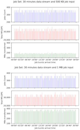
Figure 2.
Job set characteristics.
6. Metrics and Experimental Simulation Results
The scheduling heuristics’ performance is measured in terms of completed jobs, makespan, and fairness, which are metrics reported in similar distributed computing systems studies [15,16,29,30].
Completed jobs: Providing that mobile device clusters rely on the energy stored in the mobile devices’ batteries to execute jobs, scheduling technique A is considered to be more energy efficient than scheduling technique B, if the former completes more jobs than the latter with the same amount of energy. The job completion count finishes when all nodes leave the cluster, in this case, due to running out of energy.
Makespan: Measures the time the distributed system needs to complete the execution of a job set. We normalized these times duration into a 0–1 scale, where the value 1 refers to the heuristic that requires the longest makespan. To calculate the makespan, we compute the difference between the time when the first job arrives and the time when the last job is completed. To calculate the latter when all compared heuristics achieved different numbers of completed jobs, we first compute the maximum number of jobs that all heuristics completed, and use this value as a pivot to obtain the time when the last job is completed.
Fairness: The difference in energy contributed by provider nodes from the time each one joins the cluster to the time each one completes its last assigned job, is quantified via the Jain’s fairness index [31]. This index was originally used to measure the bandwidth received by clients of a networking provider but, in our case, much as by Ghasemi-Falavarjani et al. [12], Viswanathan et al. [30], it is used to measure the disparity of energy pulled by the system from provider nodes. The metric complements the performance information given by completed jobs and makespan metrics.
We ran all heuristics on 2304 scenarios with varying nodes, cluster, and job characteristics. We distinguished between older and recent clusters. Older clusters are conformed by devices with instantaneous computing capability of 300 MegaFLOPS and below, which includes the LG L9, Samsumg Galaxy S3, Acer A100, and Phillips TLE732 device models of Table 1. This is the cluster used in our previous work, see Hirsch et al. [1]. Conversely, recent clusters are conformed by the Motorola MotoG6, Samsumg A30, Xiaomi A2 lite, and Xiaomi RN7 device models with floating-point computing capability of 300 MegaFLOPS and above. Figure 3 depicts the position that each group of scenarios occupies in the heatmap representation used to display the performance values obtained for each heuristic.
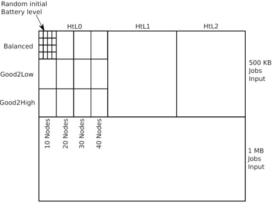
Figure 3.
Simulated scenarios: heatmap pixels.
Figure 4 shows the results of each heuristic’s completed jobs for older cluster scenarios. The darker the pixel intensity, the better is the performance achieved. Several effects of simulated variables on completed jobs are observed. First, by comparing Figure 4a,b, which show the numbers of completed jobs for AhESEAS and ESEAS, respectively, we see the magnitude of improvement introduced by the AhESEAS denominator component update policy (see Section 4). In the presence of job input above 500 KB and approximately 360 jobs generated every 12 s, which is the injected load in the scenarios, load balancing is better managed by the denominator update policy of the AhESEAS formula than that of ESEAS. AhESEAS exceeds ESEAS’s completed jobs in all scenarios. On average, the former was better than the latter by 58.6% with a standard deviation of 18.5%. Such an advantage is maintained in recent clusters scenarios, where AhESEAS (Figure 5b) is better than ESEAS (Figure 5a) by 55.2% completed jobs on average with a standard deviation of 19.1%.
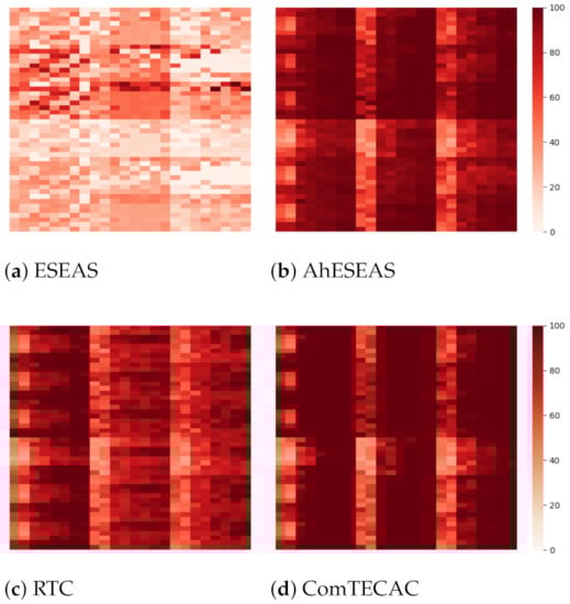
Figure 4.
Older clusters completed jobs (dark is better).
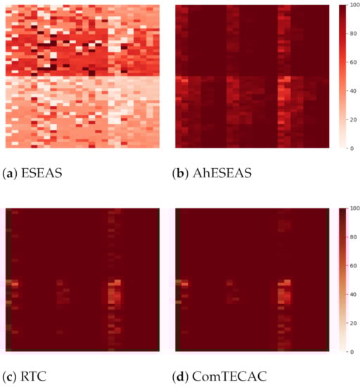
Figure 5.
Recent clusters completed jobs (dark is better).
By comparing scenario results presented at the top half and bottom half heat maps, we see the effect of job input size, i.e., completed jobs decreases as job input size increases. Such an effect is more noticeable in load balancing performed with ESEAS and AhESEAS than with the other heuristics. This indicates that job completion is not exclusively determined by how a heuristic weighs node computing capability, but also how job data and nodes’ communication-related features are included in the node ranking formula. RTC and ComTECAC include communication-related parameters in their respective node ranking formulas. RTC uses job data input/output size and node RSSI, while ComTECAC employs a function of node RSSI that relates this parameter with network efficiency. For this reason, job input size does not affect RTC and ComTECAC but certainly affects the ESEAS and AhESEAS heuristics.
Particularly, the remaining transfer capacity (RTC) heuristic [32] is instead inspired by the online MCT (minimum completion time) heuristic, which has been extensively studied in traditional computational environments such as grids and computer clusters. RTC immediately assigns the next incoming job to the node whose remaining transfer capacity is the least affected, interpreting it as the estimated capability of a battery-driven device to transfer a volume of data, considering its remaining battery level, energy cost in transferring a fixed data unit, and all jobs data scheduled in the past that waits to be transferred. At the time the remaining transfer capacity of a node is estimated, all future job output data transfers from previous job assignments are also considered.
Other variables with orthogonal effect in the number of completed jobs, i.e., observed for all heuristics, are cluster size and cluster heterogeneity. By scanning heat map results from left to right, it can seen that, for instance, in 10 nodes cluster size scenarios there are fewer completed jobs than in 20, 30, and 40 nodes cluster size scenarios. Moreover, cluster heterogeneity degrades the performance of ESEAS, AhESEAS, and RTC more than the one of the ComTECAC heuristics.
Now, focusing on overall scenario performance, when comparing the relative performance of AhESEAS and RTC, a noticeable effect emerges. In older clusters scenarios (see Figure 4), AhESEAS achieves on average higher job completion rates than RTC. RTC’s weakness in assessing the nodes’ computing capability seems to cause an unbalanced load with a clear decrease in job completion. However, this weakness seems not to be present in recent clusters scenarios (see Figure 5), where the relative performance between AhESEAS and RTC is inverted. With recent clusters, RTC’s unbalanced load is impeded by higher computing capability nodes of all recent clusters.
To finish this analysis, we can say that by taking this metric as an energy-harvesting indicator, we confirm that ComTECAC is the most energy-efficient scheduling heuristic on average. Having the same amount of energy consumption as all other heuristics, it completes more jobs in older and recent clusters simulated scenarios.
At this point, before starting to discuss other performance metrics, it is worth mentioning that due to the poor performance that ESEAS showed in terms of completed jobs, we leave it aside and focus on AhESEAS, RTC, and ComTECAC.
Figure 6 and Figure 7 depict the makespan of AhESEAS, RTC, and ComTECAC for older clusters and recent clusters scenarios. In this case, the pixels’ color intensity inversely relates to high performance, i.e., the lighter the pixel the better the performance. As explained above, where the metrics are presented, to report a comparable makespan measurement between all heuristics, we computed makespan, considering a subset of completed jobs, instead of all jobs, in the following manner. For each scenario, we determined the maximum of completed jobs for all heuristics and used this value as a reference to compute the makespan value of each heuristic. The makespan values reported in Figure 6 and Figure 7 were calculated using completed jobs of the RTC, AhESEAS, and ComTECAC heuristics. The dark blue pixels’ predominance in Figure 6a indicates that RTC was the heuristic with the overall longest makespan on average, compared to that obtained by the AhESEAS and ComTECAC heuristics. Moreover, when comparing RTC and AhESEAS, we see that one’s makespan mirrors the other, i.e., in scenarios where RTC achieves good makespan, AhESEAS obtained bad makespan values and vice versa.
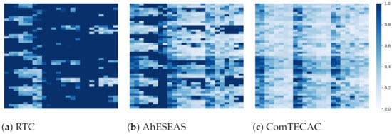
Figure 6.
Older clusters’ makespan (light is better).
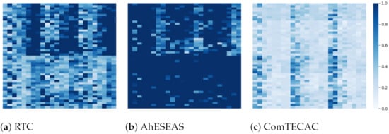
Figure 7.
Recent clusters’ makespan (light is better).
When analyzing recent clusters scenarios, shown in Figure 7a, we see the effect of device models with more computing capability on the relative performance of RTC and AhESEAS. In these scenarios, RTC achieves, on average, better makespan than AhESEAS. These results are in line with the behavior observed via the completed jobs metric. These results provide evidence on an AhESEAS node ranking formula’s weakness, which underestimates the jobs data transferring requirement in the nodes ranking formula. In summary, ranking formulas of both RTC and AhESEAS heuristics have weaknesses. By increasing clusters’ instantaneous computing capability with new device models, we see that the RTC weakness can be compensated, while the AhESEAS weakness is increasingly visible. Consistent with this affirmation, when comparing 1 MB input with 500 KB input scenarios presented in Figure 7a,b, we see that, when considering those scenarios taking the lowest time to transfer data, i.e., where jobs have 500 KB input, RTC performed worse than AhESEAS.
Job input size, cluster size, and cluster heterogeneity effects described for the completed jobs metric still apply. To finish this analysis, we may say that the ComTECAC ranking formula combines the strengths from RTC and AhESEAS, and its advantage over the other heuristics in the majority of scenarios is remarkable.
Finally, we report the performance of the heuristics using the fairness metric. Provided that the heuristics target different numbers of completed jobs for the same scenario, to calculate fairness, we followed similar initial steps as with makespan. For each scenario, we first determined the maximum number of completed jobs by all heuristics (except ESEAS), and used it as reference value to compute the fairness score. Once obtained, we searched for each heuristic for the associated time stamp when this number of completed jobs has been reached. The time stamp is another reference, in this case, to get the last battery level reported by each participating node. Then, with such data, and the initial battery level reported by each node, we computed an energy delta, i.e., the node energy contribution, which is interpreted as a sample in the fairness score calculation formula.
According to Figure 8 and Figure 9, RTC’s fairness is clearly lower than that of AhESEAS and ComTECAC, on average. In contrast, since the fairness scores of the last two heuristics are quite similar, we formulated the null hypothesis that the fairness achieved is the same. We tested with the Wilcoxon test, pairing the fairness values of AhESEAS and ComTECAC for 2304 scenarios. This resulted in a p-value of , which lead us to reject . To conclude this analysis and figure out which of the last two heuristics performed better, we re-computed the fairness metric, this time considering completed jobs only by the AhESEAS and ComTECAC heuristics. The ComTECAC fairness values shown in Figure 10b and Figure 11b are seemingly better than the ones of AhESEAS shown in Figure 10a and Figure 11a. We confirm this by complementing heat maps with a cumulative scenarios density function for older cluster scenarios in Figure 10c and recent cluster scenarios in Figure 11c. In older and recent clusters, the ComTECAC CDF increase is more pronounced than that of AhESEAS as the fairness score increases, i.e., for many scenarios, ComTECAC achieves higher fairness than AhESEAS.
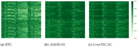
Figure 8.
Older clusters’ fairness (dark is better).
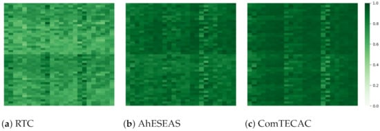
Figure 9.
Recent clusters’ fairness (dark is better).
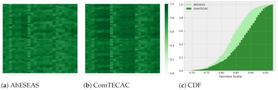
Figure 10.
Recomputed fairness considering AhESEAS and ComTECAC heuristics only (dark is better).
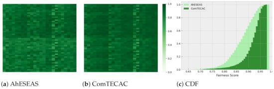
Figure 11.
Recomputed fairness for recent clusters scenarios considering AhESEAS and ComTECAC heuristics only (dark is better).
7. An Experiment of Simulating Video Processing
In spite of the experiments presented above, a question that remained unanswered was whether distributing and executing tasks that process a given stream of edge data using nearby mobile devices is actually beneficial as compared to gather and process the stream individually by smartphones. Assuming that finding a generic answer is difficult, we focus our analysis on a generic class of stream processing mobile application that might be commonplace in smart city dew contexts: per-frame object detection using widespread deep learning architectures over video streams. The goal of the experiment in this section is to simulate a realistic video processing scenario at the edge using a cluster of smartphones. We base this on real benchmark data from mobile devices performing deep learning-based object detection.
As a starting point, we took the Object Detection Android application from the Tensorflow Lite framework (https://www.tensorflow.org/lite/examples/object_detection/overview accessed on 18 August 2021). It includes a YOLO v3 (You Only Look Once) neural network able to detect among 80 different classes. The application operates by reading frames from the smartphone camera and producing a new video with annotated objects, indicating detected class (e.g., “dog”) and confidence value. We modified the application to include the newer YOLO v4 for Tensorflow Lite, which improves detection accuracy and speed, see Bochkovskiy et al. [33], and the average frame processing time since application start. A screenshot of the application is shown in Figure 12. The APK is available at https://drive.google.com/file/d/18Q5SLrKtvgsyAb_wA7QZ0TMjIM_jK9hz/view accessed on 18 August 2021.
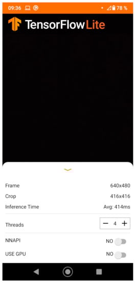
Figure 12.
Screenshot of the Tensorflow Lite modified object detection application. The dark area displays the camera input and detections..
After that, we took each smartphone belonging to the recent cluster used in the previous section, and performed the following procedure:
- 1.
- Install the APK.
- 2.
- Run a shell script that monitors CPU usage every second, and stores this measure in a log file. This script simply parses the information in the /proc/stats system file to produce CPU usage values between 0% and 100%.
- 3.
- Run the app by configuring 1 (one) thread.
- 4.
- Wait until the inference time (in milliseconds) converges.
- 5.
- Close the app, save the log file from step (2) and the inference time from step (4).
Then, we repeated steps (2)–(5) by incrementally using more threads in the device, until finding the lowest average inference time. Lastly, we processed the log files by removing the initial entries representing small values that were due to the app not yet processing camera video.
Table 6 shows the results from the procedure when applied to the recent cluster smartphones. To instantiate the DewSim simulator with Tensorflow Lite benchmark information, there was the need to convert job inference time into job operations count. This is because DewSim uses job operations count, node flops, and node CPU usage to simulate jobs completion time. To approximate the job operations count, we applied the following formula, which combines inference time, MaxFlops, and CPU usage percentage:
where is the average inference time (in seconds), is the MaxDeviceFlops (in multithread mode), and is the CPU usage percentage, which is known data derived from the benchmarking tasks described above.
Table 6.
Tensorflow Lite app on recent cluster smartphones: benchmark results.
However, jobOps varies when instantiating this formula for different device models. To feed DewSim with a unified jobOps value—in practice the same job whose completion time varies with device computing capabilities—we adjusted the DewSim internal logic to express nodes’ computing capability as a linear combination of the fastest node which was used as pivot. In this way, devices computing capability is expressed by MaxFlops multiplied by a coefficient obtained from the following linear equation system:
This adjustment allowed DewSim to realistically mimic the inference time and CPU usage as benchmarked for each device model. In addition, the energy consumption trace for the observed CPU usage in devices while processing frames in a certain device model was also configured to DewSim.
Figure 13 shows the processing power and time employed by different smartphone clusters (dew contexts) in processing 9000 jobs, which directly map to individual frames contained in a 5 min 30 FPS video stream. Each job has an input/output size of 24 KB/1 KB, respectively. The input size relates to 414 × 414 images size that the Tensorflow Lite model accepts as input. Besides, 1 KB is the average size of a plain text file that the model can produce with information of objects identified in a frame. Job distribution in all dew contexts was done via ComTECAC since, as previous experiments showed, this scheduling heuristic achieved the best performance in terms of completed jobs, makespan, and fairness metrics as compared to other state-of-the-art heuristics. Heterogeneity in all configured dew contexts is given not only by the combination of nodes with different computing capabilities but also by different initial battery levels because ComTECAC also uses this parameter to rank nodes. We configured scenarios where good battery levels (above 50%) are assigned either to fast—FastNodesWGoodBattLevel—or to slow—SlowNodesWGoodBattLevel—nodes, or they are equally distributed between fast and slow nodes—HalfFastAndSlowNodesWGoodBattLevel. Another scenario considered all nodes having the same battery level. Figure 13a reveals that dew contexts with four nodes can reduce makespan by more than half as compared to what a single instance of our fastest benchmarked smartphone is able to achieve, which means collaborative smartphone-powered edge computing for these kinds of applications is very useful. Figure 13b,c show that makespan can be considerably reduced as more nodes are present in the dew context. Particularly in a dew context with 12 nodes, see Figure 13c, near real-time stream processing is observed, where the job processing rate is scarcely a few seconds behind the job generation rate.
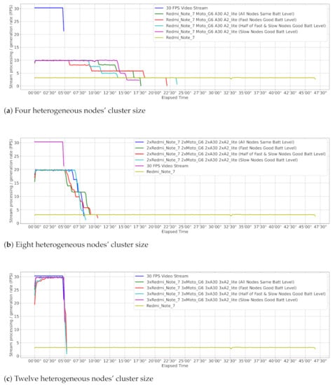
Figure 13.
Object detection using the ComTECAC scheduling heuristic over a 5-min, 30 FPS video stream.
8. Discussion
8.1. Summary of Results
From the extensive experiments performed using battery traces and performance parameters from real devices, we arrived at several conclusions about all presented heuristics. First of all, by comparing ESEAS and AhESEAS completed jobs, the performance improvement achieved when changing the denominator update policy is remarkable, i.e., the logic followed by AhESEAS of updating the queued jobs component as soon as a node is selected for executing the next job. This holds when the job input size is at least 500 KB w.r.t. updating the denominator component when the node completely receives the whole job input which is the logic to update the denominator of ESEAS. With this change, between 55.2 and 58.6% more jobs are completed on average.
In older clusters, AhESEAS completed 8.2% and 4.3% more jobs on average than the RTC heuristic in 500 KB and 1 MB data input scenarios, respectively. In contrast, for recent cluster scenarios, RTC outperformed AhESEAS by 1.46% and 3.4% of completed jobs on average in 500 KB and 1 MB data input scenarios, respectively. Besides, we see a direct relationship between completed jobs and makespan, meaning that the heuristic which beats the other, either AhESEAS or RTC, in jobs completion also achieved the relatively least makespan. Moreover, by comparing the fairness of these two heuristics in older and recent clusters scenarios, it yields that AhESEAS always behaves better than RTC.
In summary, AhESEAS and RTC show complementary behavior. Simulated scenarios where one of these achieves high performance the other targets low performance and vice-versa. Both heuristics would be needed to achieve high performance in a wide variety of scenarios.
On the contrary, ComTECAC performance is stable and high in all scenarios. For ranking nodes, ComTECAC considers communication and computing capabilities, as well as energy contribution parameters. The combination of all these allows ComTECAC to complete slightly more jobs than the second-best heuristic, between and . At the same time, ComTECAC targets considerably less makespan than its competitors. It achieves a speedup around 1.69 and 2.74 w.r.t. the second-fastest heuristic. ComTECAC is also the fairest heuristic for load balancing. In older clusters, the first 50% (median), 80%, and 90% distribution samples, present fairness values of 0.88, 0.92, and 0.94, respectively, while the second fairest heuristic for these cutting points results in fairness values of 0.84, 0.86, and 0.87, respectively. In recent clusters, the same analysis is even more in favor to ComTECAC, whose fairness values are 0.92, 0.94, and 0.95 vs. 0.88, 0.92, and 0.94 achieved by AhESEAS.
Finally, we instantiated our simulations with a practical case in which mobile devices recognize objects from video streams using deep learning models. For running these simulations, we explained the adaptations that were performed to DewSim, which represent a starting point for incorporating other benchmarked models. We conclude that close to real object detection is viable with a reasonable amount of dedicated mobile devices.
8.2. Practical Challenges
In the course of doing this work, we have identified some challenges towards exploiting the proposed scheduling heuristics in particular, and the collaborative computing scheme as a whole in general, in order to build smart cities. First, our collaborative computing scheme lacks mechanisms for promoting citizens’ participation, accounting for computing contribution, and preventing fraud in reporting results. Incentive mechanisms proposed for collaborative sensing are not applicable for resource-intensive tasks and, in fact, some research has been done on this topic [19]. Some of the questions that remain unanswered regarding these challenges are: Is the job completion event a good checkpoint for giving credits to resource provider nodes? What are the consequences of giving a fixed amount of credits upon a job completion irrespective of the time and energy employed by a device? How many results of the same job would be necessary to collect in order to prevent fraud in reporting job results? In short, apart from luring citizens into using our scheme, it is necessary to reward good users and to identify malicious ones.
Another evident challenge is that a middleware implementing basic software services for supporting the above collaborative scheme is necessary. Besides, wide mobile OS and hardware support in the associated client-side app(s) must be ensured, which is known to be a difficult problem from a software engineering standpoint. To bridge this gap, we are working on a middleware-prototype for validating our findings. We already integrated libraries that use traditional machine vision and deep learning object recognition and tracking algorithms into our device profiling platform, which is a satellite project of the DewSim toolkit. This is necessary to validate our load balancing heuristics with real object recognition algorithms, which in turn complement our battery-trace capturing method that currently exercises CPU floating-point capabilities through a generic yet synthetic algorithm. This integration also allows for deriving new heuristics to refine the exploitation of mobile devices by profiling specialized accelerator hardware such as GPUs and NPUs, which are suited for running complex AI models [22]. The first steps have been already taken using our Tensorflow-based Android benchmarking application, but we need to study how to generate GPU-aware energy traces, how to properly profile GPU hardware capabilities into indicators, and how to exploit these traces and indicators through specialized AI job schedulers.
Lastly, another crucial challenge is how to ensure proper QoS (Quality of Service) in our computing scheme considering that, in smart city applications, there is high uncertainty regarding the computing power—in terms of the number of nodes and their capabilities—available at any given moment to process jobs. The reason is that devices might join and leave a dew context dynamically. In this line, several questions arise: is it possible to predict within acceptable error margins how much time an individual device will stay connected in a dew context? For example, in certain smart city dew contexts (e.g., public transport) connectivity profiles for each contributing user could be derived by exploiting users’ travel/mobility patterns. Then, long-lasting devices could be given more jobs to execute. Another question is how to regulate job creation in a dew context, so that no useless computations are performed and, hence, higher QoS (in terms of, e.g., energy spent and response time) is delivered to smart city applications? As an extreme example, the number of jobs created from a continuous video stream in applications involving public transport should not be constant, but depend on the current speed of the bus.
9. Conclusions and Future Work
In this paper, we present a performance evaluation of practical job scheduling heuristics for stream processing in dew computing contexts. ESEAS and RTC are heuristics from previous work, while AhESEAS and ComTECAC are new. We measured the performance using the completed jobs metric, which quantifies how efficiently the available energy in the system is utilized: the makespan metric, which indicates how fast the system completes job arrivals, and the fairness metric, which measures the energy contribution differences among participating devices. The new heuristics, specially ComTECAC, had superior performance. These results present a step towards materializing the concept of dew computing using mobile devices from regular users. It will be applied to real-world situations where online data gathering and processing at the edge are important, such as smart city applications.
Despite our focus on heuristics to orchestrate a self-supported distributed computing architecture that leverages idle resources from clusters of battery-driven nodes, to extend the architecture’s applicability, new efforts will follow. We will study complementing battery-driven resource provider nodes with non-battery-driven fog nodes, e.g., single-board computers, in a similar way to other work that studied the synergy among different distributed computing layers, e.g., fog nodes and cloud providers [34].
With the goal of making our experimental methodology easier to adopt and use, another aspect involves the development of adequate soft/hard support to simplify the process of battery trace creation to feed DewSim. For instance, Hirsch et al. [35] have recently proposed a prototype platform based on commodity IoT hardware such as smart Wifi switches and Arduino boards to automate this process as much as possible. The prototype, called Motrol, supports batch benchmarking of up to four smartphones simultaneously, and provides a simple, JSON-based configuration language to specify various benchmark conditions such as CPU level, required battery state/levels, etc. A more recent prototype called Motrol 2.0, see Mateos et al. [36], extends the previous support with extra charging sources for attached smartphones (fast, AC charging and slow, USB charging) and a web-based GUI written in Angular to launch and monitor benchmarks. Further work along these lines is already on its way.
Author Contributions
Conceptualization, M.H., C.M., A.Z., T.A.M., T.-M.G., and H.K.; methodology, M.H. and C.M.; software, M.H. and C.M.; validation, M.H.; writing—original draft preparation, M.H.; writing—review and editing, C.M., A.Z., T.A.M., T.-M.G., and H.K.; visualization, M.H.; supervision, C.M. and A.Z.; funding acquisition, C.M., A.Z., and T.A.M. All authors have read and agreed to the published version of the manuscript.
Funding
This research was funded by CONICET grant number 11220170100490CO and ANPCyT grant number PICT-2018-03323.
Data Availability Statement
To obtain data and software supporting the reported results feel free to email the corresponding author.
Conflicts of Interest
The authors declare no conflict of interest.
References
- Hirsch, M.; Mateos, C.; Zunino, A.; Majchrzak, T.A.; Grønli, T.M.; Kaindl, H. A Simulation-based Performance Evaluation of Heuristics for Dew Computing. In Proceedings of the 54th Hawaii International Conference on System Sciences, Hawaii, 5–8 January 2021; p. 7207. [Google Scholar]
- Hintze, D.; Findling, R.D.; Scholz, S.; Mayrhofer, R. Mobile device usage characteristics: The effect of context and form factor on locked and unlocked usage. In Proceedings of the 12th International Conference on Advances in Mobile Computing and Multimedia (MoMM), Kaohsiung, Taiwan, 8–10 December 2014; pp. 105–114. [Google Scholar]
- Tedeschi, A.; Benedetto, F. A real-time automatic pavement crack and pothole recognition system for mobile Android-based devices. Adv. Eng. Inform. 2017, 32, 11–25. [Google Scholar] [CrossRef]
- Restuccia, F.; Das, S.K.; Payton, J. Incentive mechanisms for participatory sensing: Survey and research challenges. ACM TOSN 2016, 12, 1–40. [Google Scholar] [CrossRef]
- Gao, H.; Liu, C.H.; Wang, W.; Zhao, J.; Song, Z.; Su, X.; Crowcroft, J.; Leung, K.K. A survey of incentive mechanisms for participatory sensing. IEEE Commun. Surv 2015, 17, 918–943. [Google Scholar] [CrossRef]
- Moustaka, V.; Vakali, A.; Anthopoulos, L.G. A systematic review for smart city data analytics. ACM CSUR 2018, 51, 1–41. [Google Scholar] [CrossRef]
- Dobre, C.; Xhafa, F. Intelligent services for big data science. Future Gener. Comput. Syst. 2014, 37, 267–281. [Google Scholar] [CrossRef]
- Guo, B.; Wang, Z.; Yu, Z.; Wang, Y.; Yen, N.Y.; Huang, R.; Zhou, X. Mobile crowd sensing and computing: The review of an emerging human-powered sensing paradigm. ACM CSUR 2015, 48, 1–31. [Google Scholar] [CrossRef]
- Ali, B.; Pasha, M.A.; ul Islam, S.; Song, H.; Buyya, R. A Volunteer Supported Fog Computing Environment for Delay-Sensitive IoT Applications. IEEE IoT J. 2020, 8, 3822–3830. [Google Scholar] [CrossRef]
- Olaniyan, R.; Fadahunsi, O.; Maheswaran, M.; Zhani, M.F. Opportunistic Edge Computing: Concepts, opportunities and research challenges. Future Gener. Comp. Syst. 2018, 89, 633–645. [Google Scholar] [CrossRef] [Green Version]
- Chen, X.; Pu, L.; Gao, L.; Wu, W.; Wu, D. Exploiting massive D2D collaboration for energy-efficient mobile edge computing. IEEE Wirel. Commun. 2017, 24, 64–71. [Google Scholar] [CrossRef] [Green Version]
- Ghasemi-Falavarjani, S.; Nematbakhsh, M.; Ghahfarokhi, B.S. Context-aware multi-objective resource allocation in mobile cloud. Comput. Electr. Eng. 2015, 44, 218–240. [Google Scholar] [CrossRef]
- Wei, X.; Fan, J.; Lu, Z.; Ding, K. Application scheduling in mobile cloud computing with load balancing. J. Appl. Math. 2013, 2013, 409539. [Google Scholar] [CrossRef] [Green Version]
- Rieger, C.; Majchrzak, T.A. A Taxonomy for App-Enabled Devices: Mastering the Mobile Device Jungle. In LNBIP; Revised Selected Papers WEBIST 2017; Springer: Cham, Switzerland, 2018; Volume 322, pp. 202–220. [Google Scholar]
- Hirsch, M.; Rodríguez, J.M.; Mateos, C.; Zunino, A. A Two-Phase Energy-Aware Scheduling Approach for CPU-Intensive Jobs in Mobile Grids. J. Grid Comput. 2017, 15, 55–80. [Google Scholar] [CrossRef]
- Yaqoob, I.; Ahmed, E.; Gani, A.; Mokhtar, S.; Imran, M. Heterogeneity-aware task allocation in mobile ad hoc cloud. IEEE Access 2017, 5, 1779–1795. [Google Scholar] [CrossRef]
- Marana, P.; Eden, C.; Eriksson, H.; Grimes, C.; Hernantes, J.; Howick, S.; Labaka, L.; Latinos, V.; Lindner, R.; Majchrzak, T.A.; et al. Towards a resilience management guideline—Cities as a starting point for societal resilience. Sustain. Cities Soc. 2019, 48, 101531. [Google Scholar] [CrossRef] [Green Version]
- Mahmud, R.; Ramamohanarao, K.; Buyya, R. Application Management in Fog Computing Environments: A Taxonomy, Review and Future Directions. arXiv 2020, arXiv:2005.10460. [Google Scholar] [CrossRef]
- Hirsch, M.; Mateos, C.; Zunino, A. Augmenting computing capabilities at the edge by jointly exploiting mobile devices: A survey. Future Gener. Comput. Syst. 2018, 88, 644–662. [Google Scholar] [CrossRef]
- Hirsch, M.; Rodríguez, J.M.; Zunino, A.; Mateos, C. Battery-aware centralized schedulers for CPU-bound jobs in mobile Grids. Pervasive Mob. Comput. 2016, 29, 73–94. [Google Scholar] [CrossRef]
- Furthmüller, J.; Waldhorst, O.P. Energy-aware resource sharing with mobile devices. Comput. Netw. 2012, 56, 1920–1934. [Google Scholar] [CrossRef]
- Ignatov, A.; Timofte, R.; Kulik, A.; Yang, S.; Wang, K.; Baum, F.; Wu, M.; Xu, L.; Van Gool, L. Ai benchmark: All about deep learning on smartphones in 2019. In Proceedings of the 2019 IEEE/CVF ICCVW, Seoul, Korea, 27–28 October 2019; pp. 3617–3635. [Google Scholar]
- Silva, F.A.; Zaicaner, G.; Quesado, E.; Dornelas, M.; Silva, B.; Maciel, P. Benchmark applications used in mobile cloud computing research: A systematic mapping study. J. Supercomput. 2016, 72, 1431–1452. [Google Scholar] [CrossRef]
- Nah, J.H.; Suh, Y.; Lim, Y. L-Bench: An Android benchmark set for low-power mobile GPUs. Comput. Graph. 2016, 61, 40–49. [Google Scholar] [CrossRef]
- Luo, C.; Zhang, F.; Huang, C.; Xiong, X.; Chen, J.; Wang, L.; Gao, W.; Ye, H.; Wu, T.; Zhou, R.; et al. AIoT Bench: Towards comprehensive Benchmarking Mobile and Embedded Device Intelligence. In Benchmarking, Measuring, and Optimizing 2019; Springer International Publishing: Cham, Switzerland, 2019; pp. 31–35. [Google Scholar]
- Wilhelm, R.; Engblom, J.; Ermedahl, A.; Holsti, N.; Thesing, S.; Whalley, D.; Bernat, G.; Ferdinand, C.; Heckmann, R.; Mitra, T.; et al. The worst-case execution-time problem—Overview of methods and survey of tools. ACM Trans. Embed. Comput. Syst. (TECS) 2008, 7, 1–53. [Google Scholar] [CrossRef]
- Hirsch, M.; Mateos, C.; Rodriguez, J.M.; Alejandro, Z. DewSim: A trace-driven toolkit for simulating mobile device clusters in Dew computing environments. Softw. Pract. Exp. 2020, 50, 688–718. [Google Scholar] [CrossRef]
- Ding, N.; Wagner, D.; Chen, X.; Pathak, A.; Hu, Y.C.; Rice, A. Characterizing and modeling the impact of wireless signal strength on smartphone battery drain. ACM SIGMETRICS Perform. Eval. Rev. 2013, 41, 29–40. [Google Scholar] [CrossRef] [Green Version]
- Pandey, P.; Pompili, D. Exploiting the untapped potential of mobile distributed computing via approximation. Pervasive Mob. Comput. 2017, 38, 381–395. [Google Scholar] [CrossRef]
- Viswanathan, H.; Lee, E.K.; Rodero, I.; Pompili, D. Uncertainty-aware autonomic resource provisioning for mobile cloud computing. IEEE TPDS 2014, 26, 2363–2372. [Google Scholar] [CrossRef]
- Jain, R.K.; Chiu, D.M.W.; Hawe, W.R. A Quantitative Measure of Fairness and Discrimination; Eastern Research Laboratory, Digital Equipment Corporation: Hudson, MA, USA, 1984. [Google Scholar]
- Hirsch, M.; Mateos, C.; Rodriguez, J.M.; Zunino, A.; Garı, Y.; Monge, D.A. A performance comparison of data-aware heuristics for scheduling jobs in mobile Grids. In Proceedings of the 2017 XLIII CLEI, Cordoba, Argentina, 4–8 September 2017; pp. 1–8. [Google Scholar] [CrossRef] [Green Version]
- Bochkovskiy, A.; Wang, C.Y.; Liao, H.Y.M. Yolov4: Optimal speed and accuracy of object detection. arXiv 2020, arXiv:2004.10934. [Google Scholar]
- Elgamal, T.; Sandur, A.; Nguyen, P.; Nahrstedt, K.; Agha, G. Droplet: Distributed operator placement for iot applications spanning edge and cloud resources. In Proceedings of the 2018 IEEE 11th International Conference on Cloud Computing (CLOUD), San Francisco, CA, USA, 2–7 July 2018; pp. 1–8. [Google Scholar]
- Hirsch, M.; Mateos, C.; Zunino, A.; Toloza, J. A platform for automating battery-driven batch benchmarking and profiling of Android-based mobile devices. Simul. Model. Pract. Theory 2021, 109, 102266. [Google Scholar] [CrossRef]
- Mateos, C.; Hirsch, M.; Toloza, J.; Zunino, A. Motrol 2.0: A Dew-oriented hardware/software platform for batch-benchmarking smartphones. In Proceedings of the IEEE 6th IEEE International Workshop on Dew Computing (DewCom 2021)—COMPSAC, Huizhou, China, 12–16 July 2021; pp. 1–6. [Google Scholar]
Publisher’s Note: MDPI stays neutral with regard to jurisdictional claims in published maps and institutional affiliations. |
© 2021 by the authors. Licensee MDPI, Basel, Switzerland. This article is an open access article distributed under the terms and conditions of the Creative Commons Attribution (CC BY) license (https://creativecommons.org/licenses/by/4.0/).