
A Domain-Independent Ontology Learning Method Based on Transfer Learning


Abstract
:1. Introduction
2. Related Work
2.1. Ontology Learning
2.2. Transfer Learning
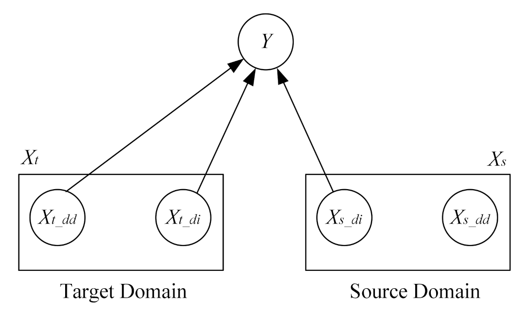
3. Problem Statement
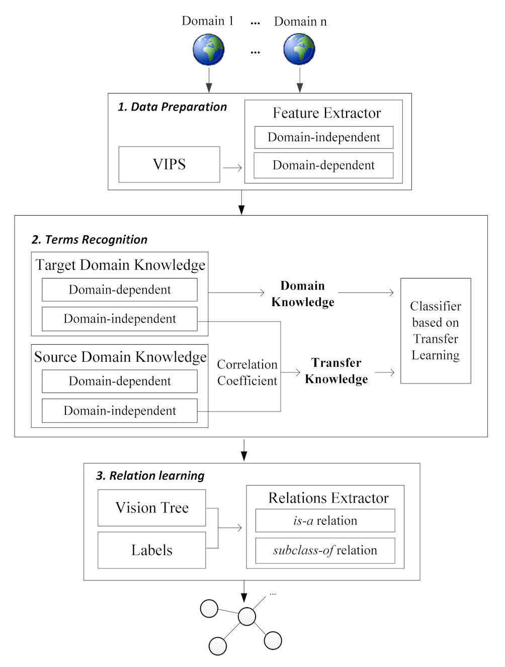
4. Model
4.1. Transfer Learning
4.2. TF-Mnt Model
4.3. Parameter Estimation
| Algorithm 1 Calculate Correlation Coefficient between and . | |
| Input: , m, n | |
| Output: ρ+ | |
| 1 | samples =[ ( , ) ] |
| 2 | for i=0 to n: |
| 3 | P_Y = distributionGen() |
| 4 | trainingSet = randomSelect(, m, P_Y) |
| 5 | = MntTrainer(trainingSet) |
| 6 | = selectGeneralW(normalize()) |
| 7 | samples.insert() |
| 8 | ρ = correlationCoefficient(samples) |
| 9 | ρ+ = setNegativeToZero(ρ) |
| 10 | return ρ+ |
5. Domain-Independent Ontology Learning
5.1. Terms Recognition by TF-Mnt
- Features from text, nine features total: the number of words, the font size, the font weight, the ratio of capital words, the location of colon, the ratio of domain concept keywords, the ratio of country keywords, the ratio of month keywords, and the ratio of all keywords.
- Features from DOM, four features total: contain URL, the location in the Web page, in <li> and in <h>.
- Features from vision tree, seven features total: the depth of the text node, the type of sibling, the type of the next node, the type of the last node, next node in <li>, last node end with colon, label of the last node. (1) Node type is inner node or leaf. (2) We use depth first search (DFS) algorithm to construct a sequence and the last or the next node means the relative location in this sequence.
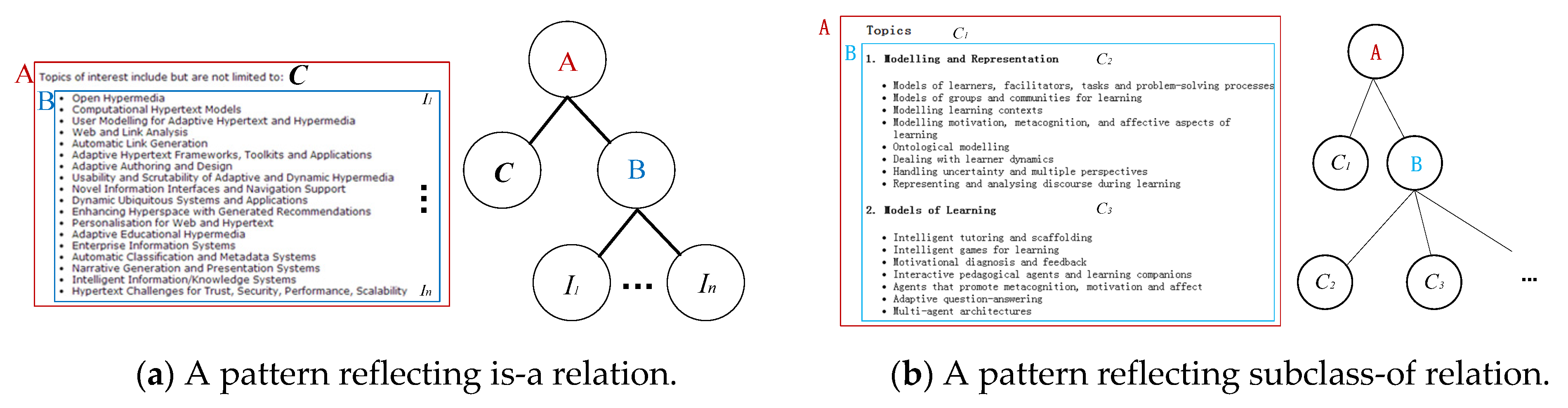
5.2. Learning of Relations by Patterns
6. Evaluation
6.1. Dataset and Settings
6.2. Results and Discussion
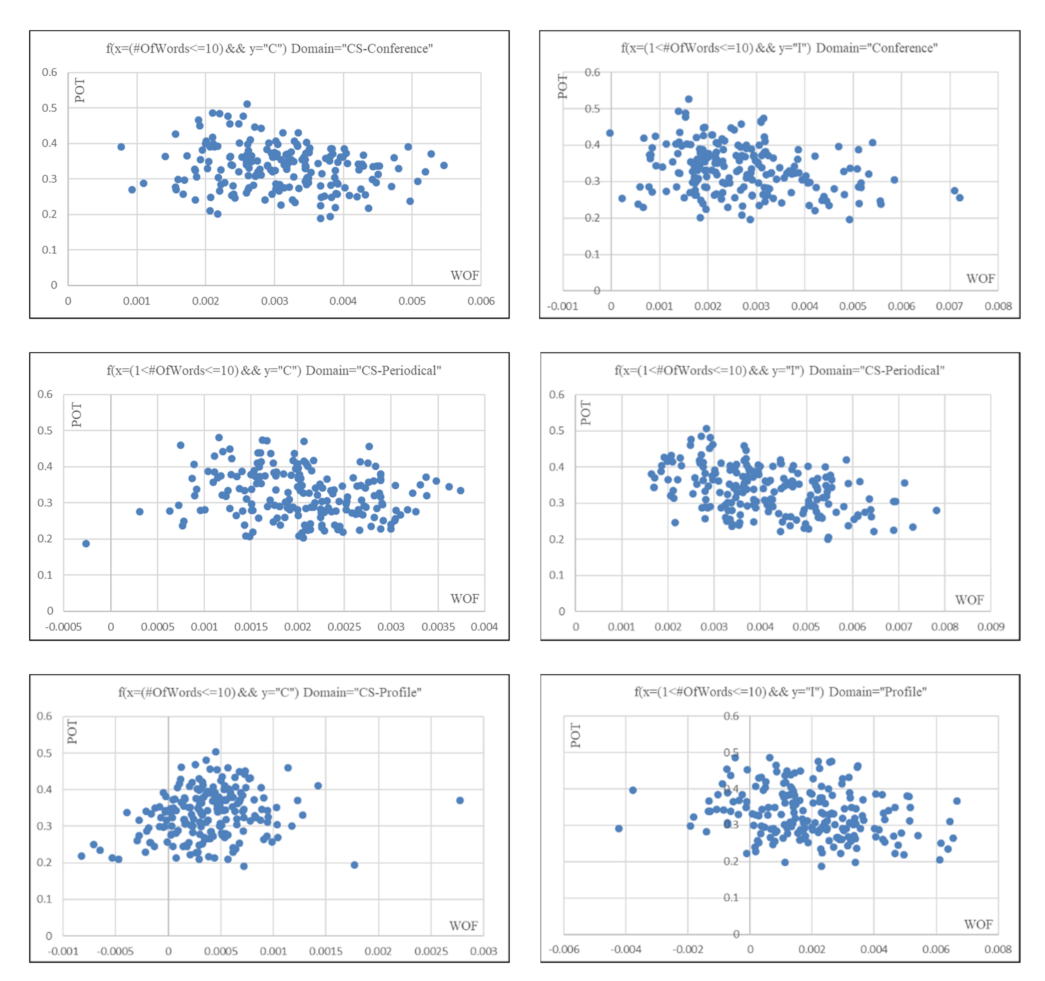
6.2.1. Effects of the Correlation Coefficient
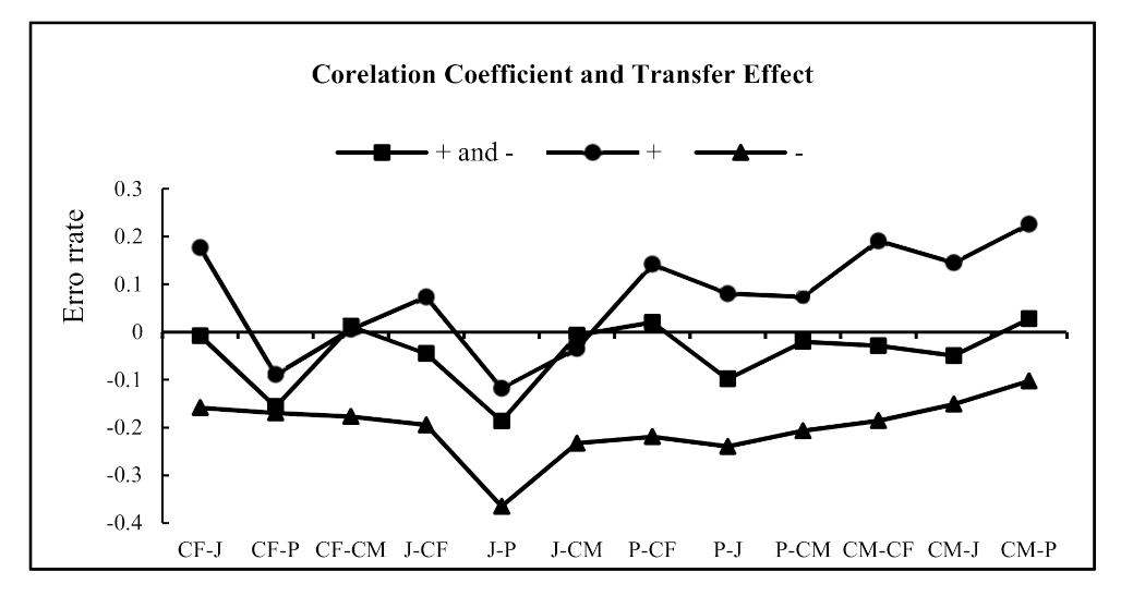
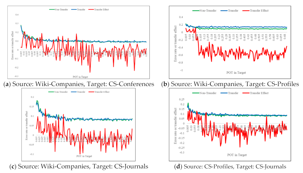
6.2.2. Effects of the Transfer Coefficient
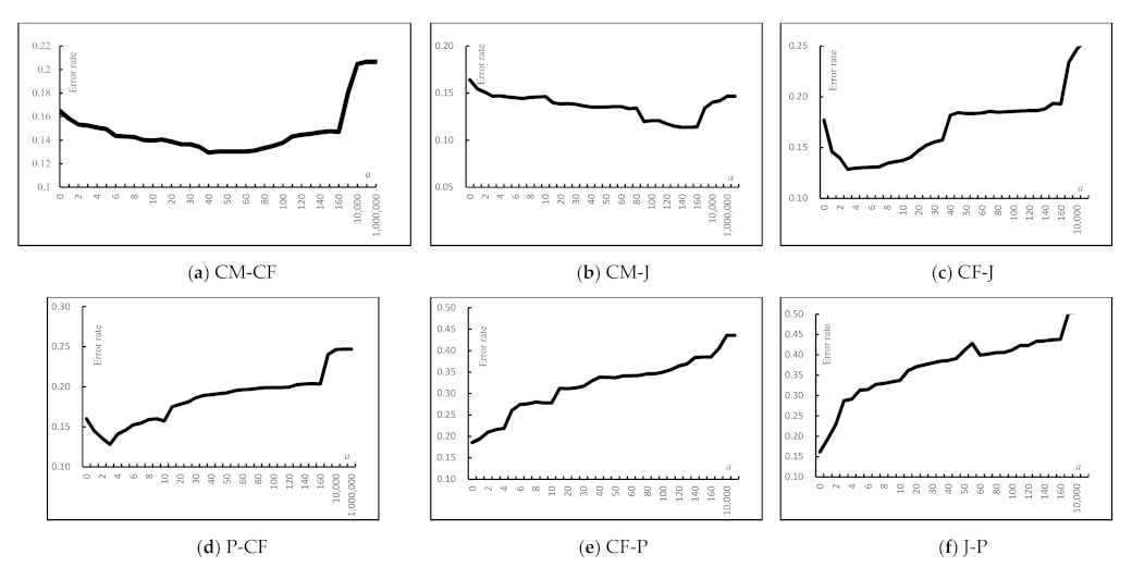
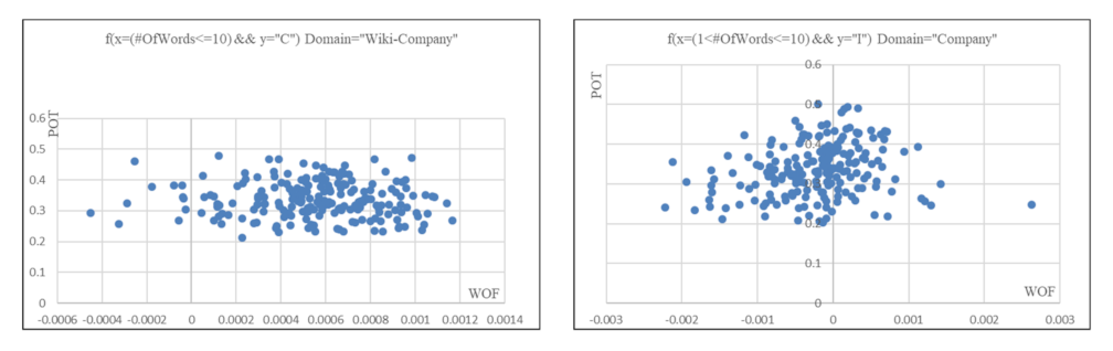
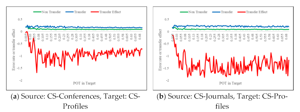
6.2.3. Effects of the Transfer Weight
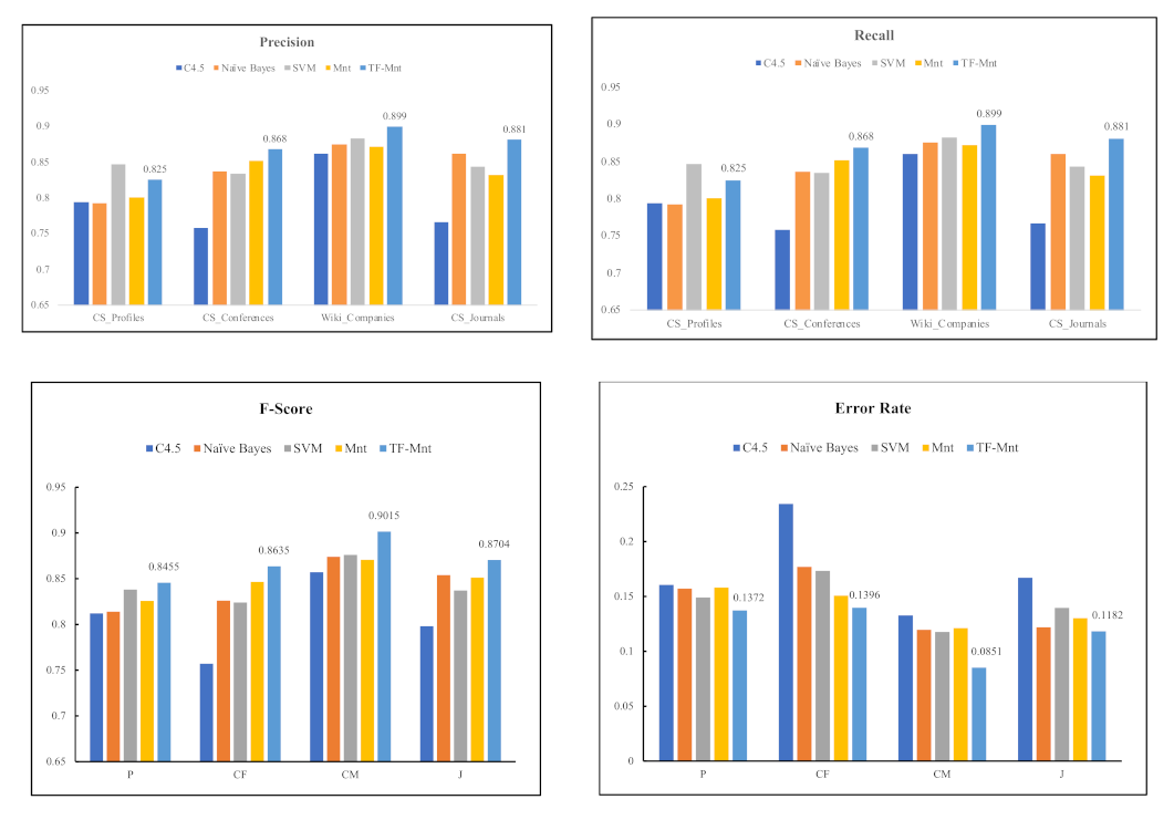
6.2.4. Model Comparison
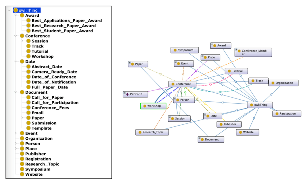
6.2.5. Ontology Learning
7. Conclusions and Future Work
Author Contributions
Funding
Conflicts of Interest
References
- McGuinness, D.L.; Van Harmelen, F. OWL Web ontology language overview. W3C Recomm. 2004, 10, 2004. [Google Scholar]
- Berners-Lee, T.; Hendler, J.; Lassila, O. The semantic Web. Sci. Am. 2001, 284, 28–37. [Google Scholar] [CrossRef]
- Dong, X.; Gabrilovich, E.; Heitz, G.; Horn, W.; Lao, N.; Murphy, K.; Strohmann, T.; Sun, S.; Zhang, W. Knowledge vault: A Web-scale approach to probabilistic knowledge fusion. In Proceedings of the 20th ACM SIGKDD International Conference on Knowledge Discovery and Data Mining, New York, NY, USA, 24–27 August 2014; 2014. [Google Scholar]
- Maedche, A.; Steffen, S. Ontology learning for the semantic Web. IEEE Intell. Syst. 2001, 16, 72–79. [Google Scholar] [CrossRef] [Green Version]
- Maedche, A.; Staab, S. Ontology learning. In Handbook on Ontologies; Springer: Berlin/Heidelberg, Germany, 2004; pp. 173–190. [Google Scholar]
- Asim, M.N.; Wasim, M.; Khan, M.U.G.; Mahmood, W.; Abbasi, H.M. A survey of ontology learning techniques and applications. Database 2018, 2018, bay101. [Google Scholar] [CrossRef] [PubMed]
- Wong, W.; Liu, W.; Bennamoun, M. Ontology learning from Text: A Look Back and into the Future. ACM Comput. Surv. 2012, 44, 20–36. [Google Scholar] [CrossRef]
- Hearst, M.A. Automatic acquisition of hyponyms from large text corpora. In Proceedings of the 15th International Conference on Computational Linguistics, Nantes, France, 23–28 August 1992. [Google Scholar]
- Pan, S.J.; Yang, Q. A survey on transfer learning. IEEE Trans. Knowl. Data Eng. 2010, 22, 1345–1359. [Google Scholar] [CrossRef]
- Cai, D.; Yu, S.; Wen, J.R.; Ma, W.Y. VIPS: A Vision-Based Page Segmentation Algorithm. Microsoft Technical Report MSR-TR-2003-79. 2003. Available online: https://www.researchgate.net/publication/243473339_VIPS_a_Vision-based_Page_Segmentation_Algorithm (accessed on 9 August 2021).
- Buitelaar, P.; Cimiano, P.; Magnini, B. (Eds.) Ontology learning from text: An overview. In Ontology Learning from Text: Methods, Evaluation and Applications; IOS Press: Amsterdam, The Netherlands, 2004. [Google Scholar]
- Wu, W.; Li, H.; Wang, H.; Zhu, K. Towards a Probabilistic Taxonomy of Many Concepts. Microsoft Technical Report MSR-TR-2011-25. 2011. Available online: https://www.researchgate.net/publication/241623566_Probase_A_probabilistic_taxonomy_for_text_understanding (accessed on 9 August 2021).
- Navigli, R.; Velardi, P. Learning domain ontologies from document warehouses and dedicated Web sites. Comput. Linguist. 2004, 30, 151–179. [Google Scholar] [CrossRef] [Green Version]
- Navigli, R.; Velardi, P. Learning word-class lattices for definition and hypernym extraction. In Proceedings of the 48th Annual Meeting of the Association for Computational Linguistics. Association for Computational Linguistics, Uppsala, Sweden, 11–16 July 2010. [Google Scholar]
- Li, F.L.; Chen, H.; Xu, G.; Qiu, T.; Ji, F.; Zhang, J.; Chen, H. AliMeKG: Domain knowledge graph construction and application in e-commerce. In Proceedings of the 29th ACM International Conference on Information & Knowledge Management, Ireland, 19–23 October 2020. [Google Scholar]
- Luo, X.; Liu, L.; Yang, Y.; Bo, L.; Cao, Y.; Wu, J.; Li, Q.; Yang, K.; Zhu, K.Q. AliCoCo: Alibaba e-commerce cognitive concept net. In Proceedings of the 2020 ACM SIGMOD International Conference on Management of Data, Portland, OR, USA, 14–19 June 2020. [Google Scholar]
- Shen, J.; Wu, Z.; Lei, D.; Zhang, C.; Ren, X.; Vanni, M.T.; Sadler, B.M.; Han, J. Hiexpan: Task-guided taxonomy construction by hierarchical tree expansion. In Proceedings of the 24th ACM SIGKDD International Conference on Knowledge Discovery & Data Mining, London, UK, 19–23 August 2018. [Google Scholar]
- Huang, J.; Xie, Y.; Meng, Y.; Zhang, Y.; Han, J. Corel: Seed-guided topical taxonomy construction by concept learning and relation transferring. In Proceedings of the 26th ACM SIGKDD International Conference on Knowledge Discovery & Data Mining, San Diego, CA, USA, 23–27 August 2020. [Google Scholar]
- Du, T.C.; Li, F.; King, I. Managing knowledge on the Web-Extracting ontology from HTML Web. Decis. Support Syst. 2009, 47, 319–331. [Google Scholar] [CrossRef]
- Wang, P.; You, Y.; Xu, B.; Zhao, J. Extracting Academic Information from Conference Web Pages. In Proceedings of the 23rd IEEE International Conference on Tools with Artificial Intelligence, Boca Raton, FL, USA, 7–9 November 2011. [Google Scholar]
- Zhu, J.; Zhang, B.; Nie, Z.; Wen, J.R.; Hon, H.W. Webpage Understanding: An Integrated Approach. In Proceedings of the 13th ACM SIGKDD International Conference on Knowledge Discovery and Data Mining, San Jose, CA, USA, 12–15 August 2007. [Google Scholar]
- Nie, Z.; Wen, J.R.; Ma, W.Y. Webpage Understanding: Beyond Page-level Search. ACM SIGMOD Rec. 2009, 37, 48–54. [Google Scholar] [CrossRef]
- Yao, L.; Tang, J.; Li, J. A Unified Approach to Researcher Profiling. In Proceedings of the Web Intelligence, IEEE/WIC/ACM International Conference on Web Intelligence, Fremont, CA, USA, 2–5 November 2007. [Google Scholar]
- Brickley, D.; Miller, L. FOAF Vocabulary Specification, Namespace Document. Available online: http://xmlns.com/foaf/0.1/ (accessed on 15 January 2021).
- Craven, M.; DiPasquo, D.; Freitag, D.; McCallum, A.; Mitchell, T.; Nigam, K.; Slattery, S. Learning to construct knowledge bases from the World Wide Web. Artif. Intell. 2000, 118, 69–113. [Google Scholar] [CrossRef] [Green Version]
- Hyoil, H.; Elmasri, R. Learning rules for conceptual structure on the Web. J. Intell. Inf. Syst. 2004, 22, 237–256. [Google Scholar]
- Mo, W.; Wang, P.; Song, H.; Zhao, J.; Zhang, X. Learning Domain-Specific Ontologies from the Web. Linked Data and Knowledge Graph; Springer: Berlin/Heidelberg, Germany, 2013; pp. 132–146. [Google Scholar]
- Gao, W.; Zhu, L.; Guo, Y.; Wang, K. Ontology learning algorithm for similarity measuring and ontology mapping using linear programming. J. Intell. Fuzzy Syst. 2017, 33, 3153–3163. [Google Scholar] [CrossRef]
- Gao, W.; Guirao, J.L.; Basavanagoud, B.; Wu, J. Partial multi-dividing ontology learning algorithm. Inf. Sci. 2018, 467, 35–58. [Google Scholar] [CrossRef]
- Zhuang, F.; Qi, Z.; Duan, K.; Xi, D.; Zhu, Y.; Zhu, H.; Xiong, H.; He, Q. A comprehensive survey on transfer learning. In Proceedings of the IEEE; IEEE: Piscataway, NJ, USA, 2020; Volume 109, pp. 43–76. [Google Scholar]
- Cai, C.; Wang, S.; Xu, Y.; Zhang, W.; Tang, K.; Ouyang, Q.; Lai, L.; Pei, J. Transfer learning for drug discovery. J. Med. Chem. 2020, 63, 8683–8694. [Google Scholar] [CrossRef]
- Rao, R.; Bhattacharya, N.; Thomas, N.; Duan, Y.; Chen, X.; Canny, J.; Abbeel, P.; Song, Y.S. Evaluating protein transfer learning with TAPE. Adv. Neural Inf. Process. Syst. 2019, 32, 9689. [Google Scholar] [PubMed]
- Pesciullesi, G.; Schwaller, P.; Laino, T.; Reymond, J.-L. Transfer learning enables the molecular transformer to predict regio-and stereoselective reactions on carbohydrates. Nat. Commun. 2020, 11, 1–8. [Google Scholar] [CrossRef] [PubMed]
- Chouhan, V.; Singh, S.K.; Khamparia, A.; Gupta, D.; Tiwari, P.; Moreira, C.; Damaševičius, R.; De Albuquerque, V.H.C. A novel transfer learning based approach for pneumonia detection in chest X-ray images. Appl. Sci. 2020, 10, 559. [Google Scholar] [CrossRef] [Green Version]
- Ruder, S.; Peters, M.E.; Swayamdipta, S.; Wolf, T. Transfer learning in natural language processing tutorial. In Proceedings of the 2019 Conference of the North American Chapter of the Association for Computational Linguistics, Minneapolis, MN, USA, 2–7 June 2019. [Google Scholar]
- Daume, H., III; Marcu, D. Domain Adaptation for Statistical Classifiers. J. Artif. Intell. Res. 2006, 26, 101–126. [Google Scholar] [CrossRef]
- Raina, R.; Ng, A.Y.; Koller, D. Constructing informative priors using transfer learning. In Proceedings of the 23rd International Conference on Machine Learning, Pittsburgh, PA, USA, 25–29 June 2006. [Google Scholar]
- Dai, W.; Yang, Q.; Xue, G.-R.; Yu, Y. Boosting for transfer learning. In Proceedings of the 24th International Conference on Machine Learning, Corvallis, OR, USA, 20–24 June 2007. [Google Scholar]
- Ling, X.; Dai, W.; Xue, G.R.; Yang, Q.; Yu, Y. Spectral domain-transfer learning. In Proceedings of the 14th ACM SIGKDD International Conference on Knowledge Discovery and Data Mining, Las Vegas, NV, USA, 24–27 August 2008. [Google Scholar]
- Dai, W.; Xue, G.R.; Yang, Q.; Yu, Y. Transferring naive bayes classifiers for text classification. In Proceedings of the National Conference on Artificial Intelligence, Vancouver, BC, Canada, 22–26 June 2007. [Google Scholar]
- Liao, X.; Xue, Y.; Carin, L. Logistic regression with an auxiliary data source. In Proceedings of the 22nd International Conference on Machine Learning, Bonn, Germany, 7–11 August 2005. [Google Scholar]
- Wu, P.; Dietterich, T.G. Improving SVM accuracy by training on auxiliary data sources. In Proceedings of the 21st International Conference on Machine Learning, Banff, AB, Canada, 4–8 July 2004. [Google Scholar]
- Hu, D.H.; Zheng, V.W.; Yang, Q. Cross-domain activity recognition via transfer learning. Pervasive Mob. Comput. 2011, 7, 344–358. [Google Scholar] [CrossRef]
- Tan, C.; Sun, F.; Kong, T.; Zhang, W.; Yang, C.; Liu, C. A survey on deep transfer learning. In International Conference on Artificial Neural Networks; Springer: Cham, Switzerland, 2018. [Google Scholar]
- Vedula, N.; Maneriker, P.; Parthasarathy, S. Bolt-k: Bootstrapping ontology learning via transfer of knowledge. In Proceedings of the World Wide Web Conference, San Francisco, CA, USA, 13–17 May 2019. [Google Scholar]
- Weiss, K.; Khoshgoftaar, T.M.; Wang, D. A survey of transfer learning. J. Big Data 2016, 3, 1–40. [Google Scholar] [CrossRef] [Green Version]
- Ratnaparkhi, A. A maximum entropy model for part-of-speech tagging. In Proceedings of the Conference on Empirical Methods in Natural Language Processing, Philadelphia, PA, USA, 17–18 May 1996. [Google Scholar]
- Nigam, K.; Lafferty, J.; McCallum, A. Using maximum entropy for text classification. In Proceedings of the IJCAI-99 Workshop on Machine Learning for Information Filtering, Stockholm, Sweden, 31 July–6 August 1999. [Google Scholar]


| Domain | C | N | I | Total |
|---|---|---|---|---|
| CF | 578 | 417 | 1261 | 2256 |
| J | 437 | 186 | 1796 | 2419 |
| P | 562 | 329 | 3503 | 4394 |
| CM | 1557 | 512 | 5636 | 7705 |
| Total | 3134 | 1444 | 12,196 | 16,774 |
| Domain | CS-Journals | CS-Conferences | Wiki-Companies | CS-Profiles |
|---|---|---|---|---|
| CS-Journals | - | 0.2550 | 0.0252 | −0.0174 |
| CS-Conferences | 0.2550 | - | −0.0860 | −0.1042 |
| Wiki-Companies | 0.0252 | −0.0860 | - | −0.0252 |
| CS-Profiles | −0.0174 | −0.1042 | −0.0252 | - |
| Domain | CS-Journals | CS-Conferences | Wiki-Companies | CS-Profiles |
|---|---|---|---|---|
| CS-Journals | - | 0.2875 | −0.0579 | −0.0315 |
| CS-Conferences | 0.2875 | - | −0.0753 | −0.0781 |
| Wiki-Companies | −0.0579 | −0.0753 | - | 0.1319 |
| CS-Profiles | −0.0315 | −0.0781 | 0.1319 | - |
| Domain Selection | Transfer Coefficient | Transfer Effect |
|---|---|---|
| J-CM | −0.0680 | −0.0347 |
| CF-CM | −0.0468 | 0.0056 |
| P-CM | −0.0413 | 0.0992 |
| J-P | −0.1017 | −0.1179 |
| CF-P | −0.0760 | −0.0892 |
| CM-P | −0.0399 | 0.2258 |
| P-CF | −0.1167 | 0.1419 |
| J-CF | −0.0958 | 0.0733 |
| CM-CF | −0.0645 | 0.1906 |
| CF-J | −0.0808 | 0.1766 |
| P-J | −0.0700 | 0.0802 |
| CM-J | −0.0645 | 0.1447 |
| Domain | is-a Relation | subclass-of Relation | Ontology Learning | ||||||
|---|---|---|---|---|---|---|---|---|---|
| P | R | F | P | R | F | P | R | F | |
| CF | 0.894 | 0.911 | 0.902 | 0.754 | 0.760 | 0.757 | 0.873 | 0.866 | 0.869 |
| J | 0.835 | 0.918 | 0.874 | 0.743 | 0.768 | 0.755 | 0.850 | 0.875 | 0.862 |
| P | 0.918 | 0.907 | 0.912 | 0.890 | 0.689 | 0.745 | 0.895 | 0.843 | 0.868 |
| CM | 0.943 | 0.899 | 0.920 | 0.785 | 0.531 | 0.633 | 0.896 | 0.791 | 0.837 |
| Avg. | 0.897 | 0.909 | 0.902 | 0.773 | 0.687 | 0.722 | 0.879 | 0.844 | 0.859 |
Publisher’s Note: MDPI stays neutral with regard to jurisdictional claims in published maps and institutional affiliations. |
© 2021 by the authors. Licensee MDPI, Basel, Switzerland. This article is an open access article distributed under the terms and conditions of the Creative Commons Attribution (CC BY) license (https://creativecommons.org/licenses/by/4.0/).
Share and Cite
Xie, K.; Wang, C.; Wang, P. A Domain-Independent Ontology Learning Method Based on Transfer Learning. Electronics 2021, 10, 1911. https://doi.org/10.3390/electronics10161911
Xie K, Wang C, Wang P. A Domain-Independent Ontology Learning Method Based on Transfer Learning. Electronics. 2021; 10(16):1911. https://doi.org/10.3390/electronics10161911
Chicago/Turabian StyleXie, Kai, Chao Wang, and Peng Wang. 2021. "A Domain-Independent Ontology Learning Method Based on Transfer Learning" Electronics 10, no. 16: 1911. https://doi.org/10.3390/electronics10161911
APA StyleXie, K., Wang, C., & Wang, P. (2021). A Domain-Independent Ontology Learning Method Based on Transfer Learning. Electronics, 10(16), 1911. https://doi.org/10.3390/electronics10161911